INTEGRATED CUTTING MACHINE PROGRAMMING AND LOT SIZING IN FURNITURE INDUSTRY Silvia Grandi dos Santos

(1)

Rio de Janeiro, v.3, n.1, p. 1-17, janeiro a abril de 2011

INTEGRATED CUTTING MACHINE PROGRAMMING AND LOT SIZING IN

FURNITURE INDUSTRY

Silvia Grandi dos Santos

silviagsantos@uel.br

Departamento de Matemática – Centro de Ciências Exatas Universidade Estadual de Londrina

Silvio Alexandre de Araujo

saraujo@ibilce.unesp.br

Socorro Rangel

socorro@ibilce.unesp.br

Departamento de Ciências da Camputação e Estatística

Instituto de Biociências, Letras e Ciências Exatas –campus de São José do Rio Preto UNESP-Universidade Estadual Paulista

Resumo

Neste trabalho, é apresentado um modelo matemático que combina problemas de dimensionamento de lotes e corte de estoque numa indústria moveleira. O modelo considera as decisões habituais de problemas de dimensionamento de lotes, bem como decisões operacionais relacionadas à programação da máquina de corte. Para resolver os problemas são usados dois conjuntos de padrões de cortes criados a priori, os padrões usados pela indústria e padrões de corte n-grupos. Também foi testada uma estratégia para melhorar a utilização da capacidade de corte da máquina. Foi utilizado um pacote comercial de otimização para resolver os problemas e os resultados computacionais, usando dados reais de uma fábrica de móveis, mostram que a utilização de um conjunto menor de padrões de corte fornece bons resultados e que a estratégia proposta é útil para aumentar a produtividade da máquina de corte.

Palavras-Chave: Problema de Dimensionamento de Lotes, Problema de Corte de Estoque, Problema Integrado, Indústria Moveleira.

Abstract

In this paper a mathematical model that combines lot-sizing and cutting-stock problems applied to the furniture industry is presented. The model considers the usual decisions of the lot sizing problems, as well as operational decisions related to the cutting machine programming. Two sets of

a priori generated cutting patterns are used, industry cutting patterns and a class of n-group cutting patterns. A strategy to improve the utilization of the cutting machine is also tested. An optimization package was used to solve the model and the computational results, using real data from a furniture factory, show that a small subset of n-group cutting patterns provides good results and that the cutting machine utilization can be improved by the proposed strategy.

(2)

PESQUISA OPERACIONAL PARA O DESENVOLVIMENTO

1 Introduction

The Furniture industry in Brazil, although spread around the country, is concentrated in regional centers, mostly situated in the south and southeast regions (Valença et al. (2002)). Each regional center includes companies of different sizes and specialties. This study is motivated by a small sized furniture factory (thereafter called Plant V) located in the northwest region of São Paulo state, which is included in the regional center of Votuporanga. Considered one of the four most important in Brazil (Landi and Gusmão (2005)), this regional center has attracted the attention of many researches (e.g. Silva (2003), Stipp (2002), Suzigan (2000), Rangel and Figueiredo (2006, 2008), Silva et al. (2007) and Mosquera and Rangel (2007)).

The Plant V is specialized in the production of bedroom furniture which is manufactured using wooden plates of different sizes and types. The production system at Plant V is very similar to that of other plants in the region. At the beginning of the week the production manager decides which types of furniture and how many will be produced during that week. The production line is then fully dedicated to these products. At first (cutting stage) the rectangular wooden plates in stock (plates) are divided into rectangular smaller pieces (pieces) that will compose a given type of furniture. The pieces are then manually processed to gain non-rectangular shapes according to the product design and pass through several other stages (e.g. gluing, drill, painting) before they are grouped to compose a final product, packed (mounted or not) and stored. There is not much space for storage of the final product, nor to store the pieces that will not be processed during the working day.

The process of cutting the plates may involve loss of material, that is, pieces that are cut and are not part of the demand. The factory is interested in reducing these losses given that they have a strong impact in the costs of the final product. One way of reducing these losses is increasing the number of demanded pieces and the demand. More pieces types may allow a better arrangement of the pieces in the plate (cutting pattern). Moreover, increasing the pieces demand might help to reduce the number of setups due to the fact that more plates may be cut simultaneously with the same cutting pattern. All this can be achieved if the industry anticipates the production of some final products. However, the anticipation of production may incur in additional inventory costs. To capture all these elements in the decision process, cutting stock and lot sizing, a combined decision should be taken. This motivated us to propose a mathematical model that combines both, the cutting-stock and the lot-sizing problems. The objective is to build a computational tool that might help the production and scheduling decisions of small and medium-sized furniture factories

(3)

present mixed integer optimization models to represent the combined cutting-stock and lot-sizing problem in the furniture industry. Gramani and França (2006) proposed a solution method based on an analogy with the network shortest path problem, Gramani et al. (2009) extended the model proposed in 2006 by considering the decisions about the final products. Some other papers that deal with the cutting stock problem in furniture industry are Yanasse et al. (1991), Carnieri et al. (1994), Morabito and Arenales (2000) and Rangel and Figueiredo (2008).

The mathematical model proposed in this paper is based on a rolling horizon planning. The model for the combined problem, besides considering capacity constraints as in Gramani and França (2006), Gramani et al. (2009) and Silva et al. (2007), also considers operational details of the cutting machine such as setup time for changes on the cutting pattern to be cut and limited thickness capacity. In the next section the production process of the furniture factory studied is described, and the proposed mixed integer model is presented. A computational study using real data from Plant V is described in Section 3, and final remarks are given in Section 4.

2 Methodology

In this section we describe the details of the production process of Plant V and the proposed mathematical model. All the plates have unlimited stock, fixed dimensions L x W (where L is the length and W is the width) and only differ by their thickness.

Due to setup constraints the factory can only produce final products that belong to the same group, where the groups are defined according to similarities in the machines configurations. For example, wardrobes with three, four and five doors belong to one group and chests and bedside tables belong to another group.

According to Yanasse et al. (1993), a cutting machine cycle is the set of operations necessary to cut one or more plates, simultaneously according to the same cutting pattern. The cutting machine is a bottleneck for the production process and some actions are considered in order to accelerate the cutting process. The cutting machine has a thickness limit so it is necessary to try to use this capacity as much as possible and to do so, several plates can be cut at the same time at each cutting machine cycle according to the same cutting pattern. It is important to consider this possibility in the decision process. A study of this aspect associated to the cutting stock problem in the context of furniture industry can be found in Mosquera and Rangel (2007).

The planning horizon considered is five periods, each period corresponding to one working day. The order book is changeable, being updated daily, so that the only decisions that are actually implemented are those of the first day. Production in later periods is only represented so that its impact on the first period decisions can be taken into account. The reality of such a rolling horizon use of lot sizing models is motivated by the following questions: why specify detailed schedules for later periods if they are never implemented? Why not use a simplified representation for later periods in the rolling horizon that would be less difficult to solve and hence permit the solution of larger problems? Several authors have pursued this approach. Stadtler (2003) and Clark (2003) showed that this flexible approach can handle large multi-level MRP-type problems over long planning horizons with sequence-independent and sequence-dependent setup times. Suerie and Stadtler (2003) used the same approach tested on smaller problems with a tight reformulation and valid inequalities providing very good and fast solutions.

In this paper, a mathematical model that captures the above ideas is proposed. As in Araujo et al.

(4)

period it is possible to know, for example, exactly how many plates must be cut according to each cutting pattern. For the other periods the decision process is less detailed.

Before presenting the mathematical modelling, a formal description of the decision process based on rolling horizon is given. Consider the following definitions from the General Lot-Sizing and Scheduling Problem (GLSP) model proposed by Fleischmann and Meyr (1997) and presented in Drexl and Kimms (1997):

t Number of sub-periods in period t



t1 1 =

τ t

=

1 +

η

F



∑

The first sub-period in period t. Note that F1 = 1

Lt = Ft +t-1 The last sub-period in period t. Note that L1=1





 T 1 t t



_{Total number of sub-periods}_{over periods 1,…,}_T

In this paper, a period t corresponds to a workday and in this case t is the number of cycles that the cutting machine can process in period t.

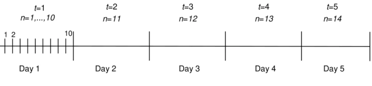
Consider a planning horizon of T = 5 workdays of which only the first day (t = 1) will be scheduled in detail. This is achieved by dividing the first day, for example, into 1=10 sub-periods, as up to 1 cutting machine cycles can be processed at first day. The remaining days t=2,...,5 have just one sub-period each (2=3=4=5=1). Thus F1= 1; L1= 10; F2= 11 = L2; F3 = 12 = L3; F4 = 13 = L4; F5= 14 =

L5, i.e., there are =14 sub-periods (as illustrated in Figure 1).

Figure 1: Periods and sub-periods in a rolling horizon strategy.

Only the scheduled decisions relative to the 1=10 sub-periods of day 1 are actually implemented. The decisions for the remaining 4 days are used only to evaluate the impact of future available capacity, i.e., to identify a provisional production plan in order to have advance warning of possible production backlogs and be able to act accordingly. Under standard rolling horizon practice, the model is reapplied one period later covering periods t = 2,…, T+1 with updated demand data over the rolled-forward T-period horizon, then over periods t= 3,…, T+2, and so on, using fresh demand forecasts (Clark (2005)).

An important aspect considered by the production manager of Plant V is the safety stock of some final products that have regular demand. The inventory levels of these final products should be

higher than a minimum level given by

s

_i. If the level of inventory for an specific item i is below

s

_i, the

production of this item must have a strong production priority over the other items. On the other hand the Plant V has limited physical space for inventory of final products and based on this limit the production

10

Day 1 Day 2 Day 3 Day 4

1 2

t=1

n=1,...,10

Day 5

t=2

n=11

t=3

n=12

t=4

n=13

t=5

(5)

manager defined a maximum desired level for each item given by

S

_i. This maximum level is also

considered the ideal level of stock because it allows attending high unexpected demand which is

important in a competitive market. It is possible to store more than

S

_i, for instance using a third-party

physical space, but paying a higher inventory cost.

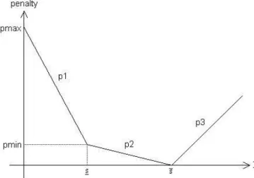
In order to consider these aspects on the decision process, a piecewise linear penalty function is considered whose value depends on the inventory level. The inventory cost value is set to high values when the inventory level is below the lower bound and is zero when it is at the upper bound. Moreover, it increases when the inventory level is above the upper bound. Figure 2 illustrates the piecewise linear penalty function used to model the inventory costs.

Figure 2: Illustration of the piecewise linearpenalty function for the inventory level of final product.

A common practice for the solution of piecewise linear problems consists of transforming them into equivalent linear programming problem (Cavichia and Arenales (2000)). In order to keep the

linearity of the model, three new variables are defined

I

_it1,

I

_it2 and

I

_it3 . If Iit is the inventory level of the

final product i in period t then Iit=

3 it 2 it 1

it

+

I

+

I

, with

0 

I

it1



s

_i ; i i 2

it

S

s

I

0 





and

I

_it3



0

. If

i 1 it

<

s

I

then, at the optimal solution,

I

_it2=0 and

I

_it3=0. On the other hand, if

0 <

I

_it2

<

S

_i



s

_i then, at

optimality, i 1 it

=

s

I

and

I

it3 =0. Finally, if 3 it

I

>0 then, at the optimal solution, i 1 it

=

s

I

and

i i 2

it

=

S

s

I



.

It is not an easy task to determine the parameters that define this piecewise linear penalty function. To generate the model instances described in Section 4 the values were defined heuristically considering the production manager opinion and the computational tests. The parameters pmax is based on the costs (including setup costs) that the plant V would have with the production of new final products to suit purchase orders if the inventory level is zero and pmin is the cost that the plant would have to supplement an order when the inventory level of a final product is low. The functions p1, which depends

only on variable

I

1_it, p2, which depends only on variable

I

_it2 , and p3, which depends only on variable

3 it

I

were linearized using the parameters pmin and pmax thus obtained. Finally, it is worth observing that

(6)

2.1 Mathematical Model

A mathematical model for the furniture production process is presented next. It is worth noting that although it is based on the production process of Plant V, it can be useful to other furniture factories with similar production processes. Consider that the following indices, data and variables are known.

Indices: t = 1,..., T periods (workdays);

i = 1,..., M final products;

p = 1,..., P pieces;

k = 1,..., K plates (each plate has different thickness);

j = 1,..., Nkcutting patterns for the plate k;

τ= F1,..., LT sub-periods (cutting machines cycles);

m = 1,...,  machines (except the cutting machine);

l = 1,...,  final product groups;

Data:

i

S

Upper bound for the security inventory level of the final product i;

i

s

Lower bound for the security inventory level of the final product i;

pmax Maximum penalty value to the inventory level of final product i;

pmin Penalty value to the inventory level of final product i when it is on the minimum security level;

p1(

I

it1) Penalty function given by

I

+

pmax

s

pmax

=

)

(I

p1

it1

i 1

it



;

p2(

I

it2) Penalty function given by

I

+

pmin

s

S

pmin

=

)

(I

p2

_it2

i i 2

it



;

p3(

I

_it3) Penalty function given by p3(I_it3)=



I_it3where



is a positive

angular coefficient;

cpkj Cost of material loss (per cm2) when the plate k is cut according to the cutting pattern j;

cdit Production cost of the final product i in period t;

k pt

SIP Inventory level capacity of pieces p cut from plate k in period t;

dit Demand for final product i in period t;

rk_pi Number of pieces p cut from plate k to produce one unit of the final product i;

a_pjk Number of pieces p cut from plate k according to the cutting pattern

j;

G Set of products that can be produced together in a workday (group);

C Thickness capacity of the cutting machine (mm); k Thickness of the plate k;

(7)

tci Time necessary to cut all the pieces to produce one unit of the final product i;

tpi Time necessary to process all the pieces to produce one unit of the final product i in the other machines (except the cutting machine);

vj Time necessary to cut one plate, or more, according to the cutting pattern j;

m pk

α Time necessary to process a piece p from a plate k in the machine

m;

csjτ Cutting machine setup cost for the cutting pattern j in sub-period τ;

CSt Capacity available on the cutting machine in period t;

Capt Aggregated capacity available on the others machines (except the cutting machine) in period t;

CMmt Capacity available on the machine m in period t (except the cutting machine);

 Large real number;

Variables: Xit Number of final products (lot-size) i to be produced in period t;

1 it

I

Inventory of the final product i in period t, below the lower bound;

2 it

I

Inventory level of the final product i in period t, between the lower

bound and the upper bound; 3

it

I

Inventory level of the final product i in period t, above the upper

bound;

IPkpt Inventory level of pieces p cut from plate k in period t;

Ykjτ Number of plates k to be cut according to the cutting pattern j in

sub-period τ;

zkjτ Binary variable: zkjτ=1 if the cutting machine is configured to cut

the plate k according to the cutting pattern j in sub-period τ, otherwise zkjτ=0;

Zkjτ Binary setup variable: Zkjτ = 1 if there is a machine changeover to

cut the plate k according to the cutting pattern j in sub-period τ, otherwise Zkjτ = 0;

Qlt Binary variable: Qlt =1 if the production process is configured to cut pieces for final products in the group l in period t, otherwise

Qlt=0;

(8)

     















 M 1 = i K 1 = k k N 1 = j L 1 F

τ= kj kjτ jτ kjτ

T 1 = t M 1 i T 2 = t it it 3 it 2 it 1 it 1 Z cs + Y cp + X cd + I p3 + I p2 + I p1

Min ₍₁₎

subject to: 3 it 2 it 1 it it it 3 1 t i, 2 1 t i, 1 1 t

i,

+

I

+

I

+

X

=

d

+

I

+

I

+

I

_ _ _

i=

1 ,



M,

t=

1 ,



,T

(2)



k





N j= L τ=F kp M i= i k pi kjτ k pj

kp

+

a

Y

=

r

X

IP

1 1 1 1 1 1

0

k=

1 ,



,K,

p=

1 ,



,P

k (3)





 

K 

1 = k k N 1 = j 1 1 L 1 F =

τ j kjτ j kjτ CS Z ts + z v (4)





      K 1 k= k P 1 p= 1 m M 1 i= 1 i k pi k

pm r X CM

α

m=

1 ,



,

Π

(5)

t M

1 i=

it i

X

CS

tc





t=

2 ,



,T

(6)

t M

1 i=

it i

X

Cap

tp





t=

2 ,



,T

(7)

i i 2 it i 1

it s and I S s

I   

i=

1 ,



,M,

t=

1 ,



,T

(8)

k 1 p 1 kp SIP

IP 

k=

1 ,



,K,

p=

1 ,



,P

_k (9)







l i lt it

μ

Q

X

l



G,

t=

1 ,



,T

(10)







G l lt

1 Q

_t=

₁

_,

_

_,T

₍₁₁₎



K 

1 = k k N 1 j= kjτ 1

z

τ

=

F

₁

,



,L

₁ (12)

kjτ k kjτ

_ε

z

C

Y

_













k

=

1 ,



,K,

j=

1 ,



,N

k

,

τ=F

1

,



,L

1 ₍₁₃₎

1 -τ kj, kjτ kjτ

z

Z





k

=

1 ,



,K,

j=

1 ,



,N

k

,

τ=F

1

,



,L

1 ₍₁₄₎

0 I

,

I

,

I

,

X

it3

2 it 1 it

it



i=

1 ,



,M,

t=

1 ,



,T

(15)

0 IP

_kpt



k

=

1 ,



,K,

p=

1 ,



,P

_k

,

t=

1

(16)

 

0,1

z

integer,

0 Y

0,

Z

kjτ



kjτ



kjτ



k 1 1

,L

,

τ=F

,

,N

,

1 j=

,K,

,

1 =

k



(17)

 

0,1

(9)

The objective function (1) minimizes the sum of inventory costs (and penalties) over all periods, production costs from the beginning of the second period, loss of material and setup costs for the first period. Constraints (2) balance final product inventories, demand and production in each period. The constraints (3) are only defined for the first period and balance piece inventories, demand and production. These constraints are the only ones that integrate the lot sizing (Xit variables) and cutting stock (Ykjτ variables) decisions.

Constraint (4) is also only defined for the first period and keeps production within the cutting machine’s capacity, considering the time to cut each pattern (which depends on the cutting pattern) and setup time of the cutting machine. Observe that due to constraints (14) the setup time is considered only if there is a change in the cutting pattern from one sub-period to another. The aggregated capacity constraints for all the other machines (except the cutting machine) in period one are considered in (5). The set of constraints (6) and (7), are the capacity constraints for the cutting machine and the aggregated capacity constraints for all the other machines from period two. These constraints are important for the first-period decisions because it is necessary to take into account possible early production in order to meet the demand in future periods.

The constraints (8) limit the final product inventory level of each type of inventory variable. The constraint (9) is only defined for the first period and keeps the inventory of the pieces within an appropriated level. Without loss of generality the initial inventory level of the final products and pieces are set to zero. The constraints (10) and (11) ensure that only final products of the same group are produced in each period and that at most one group can be produced in one period.

By the constraints (12) only one type of cutting pattern can be cut on the cutting machine at each sub-period so that each sub-period is a cutting machine cycle. Moreover, the constraints (13) ensure that the quantity of plates cut simultaneously according to a cutting pattern is limited to the cutting machine thickness capacity. In the computational tests, we compare the results of the constraints (13) with the optional constraints (19) where a lower bound is considered in order to try to improve the cutting machine utilization and to reduce the number of the cutting machine cycles.

)

19 (

L

,

F

=

τ

,

N

,

1,

=

j

K,

,

1,

=

k

z

ε

C

Y

z

1 ε

C

1 1 k kjτ k kjτ kjτ k











































As zkjτ-1 and zkjτ are both binary variables, constraints (14) and the objective function (1) force the variable Zkjτ to have value 1 if there is a changeover from a cutting pattern to a different one and,

along with constraints (17), to have value 0 otherwise. Thus Zkjτ =1 if zkjτ-1 = 0 and zkjτ = 1; Zkjτ = 0 if zkjτ

-1=zkjτ =0 or zkjτ-1=zkjτ =1 and the variable Zkjτ can be relaxed to be continuous. Finally, the constraints (15)-(18) define the type of each variable.

3 Analysis and Discussion of the Results

(10)

sequence-PESQUISA OPERACIONAL PARA O DESENVOLVIMENTO

dependent. The production costs (used from period 2 to period T ) were defined based on the sale price minus de profit margin of the final products.

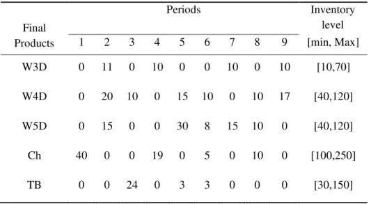
The five final products are divided in =2 groups according to the plant practice. Group one is composed of three types of wardrobes (W3D, W4D, W5D) and group two is composed of chests and table beds (Ch, TB). Table 1 shows the forecast demand (dit) for these five products and the desired

inventory level (

s

_i and

S

i) considering a planning horizon of 9 periods (working days), although only

the first five periods are of interest. The demand for the remaining four periods is important for the rolling horizon strategy used to solve the model.

The two instances generated differ in the number and type of cutting patterns used. In a preliminary version of this paper (Araujo et al. (2008a)), two sets of cutting patterns generated a priori

were used. The first one contained 61 manually generated cutting patterns used by Plant V. The second one contained 1180 composed checkboard patterns (a class of n-group cutting patterns) generated by the heuristic HTC (Rangel e Figueiredo (2008)). Due to feasibility difficulties, the inventory level capacity of

pieces p, SIP_ptk, was set to high values.

In this paper we found a better balance in the number and type of cutting patterns used to generate the two instances. One instance (MCP_V) contains 61 homogeneous cutting patterns (cutting patterns built with only one type of piece) plus the 61 manually generated cutting patterns used by Plant V. The other instance (MCP_H) contains the same homogenous cutting patterns used in instance MCP_V plus 26 cutting patterns, out of the 1180 cutting patterns generated by the heuristic HTC, which belongs to the optimal basis for the pure cutting stock problem. The inclusion of the homogeneous cutting patterns

in both instances allowed a reduction in the value of SIP_ptk. The necessary time (vj) to cut one plate, or

more, according to the Plant V, Homogeneous and HTC cutting patterns is 4.5 minutes.

Table 1: Demands and desirable inventory levels

Final Products

Periods Inventory

level

1 2 3 4 5 6 7 8 9 [min, Max]

W3D 0 11 0 10 0 0 10 0 10 [10,70]

W4D 0 20 10 0 15 10 0 10 17 [40,120]

W5D 0 15 0 0 30 8 15 10 0 [40,120]

Ch 40 0 0 19 0 5 0 10 0 [100,250]

TB 0 0 24 0 3 3 0 0 0 [30,150]

The model was coded using the Xpress-Mosel modeling language and the instances solved by the Xpress-MP solver (Dash (2009)) using an AMD Athlontm 64X2 Dual Core machine with 2,8 GHz and 2 GB RAM under Windows XP. The instance MCP_V, that uses 122 cutting patterns, has 95,688 variables and 11,630 constraints and the instance MCP_H, that uses 87 cutting patterns, has 68,477 variables and 11,032 constraints. Note that in the computational tests the integer variables Ykjτ were

(11)

According to the rolling horizon strategy, each instance is solved five times. In the first run, periods 1 to 5 are considered, in the second run the periods 2 to 6, and so on up to the fifth run in which the periods 5 to 9 are considered. The cutting machine capacity is considered in detail only in the first period of each run, that is periods 1, 2, 3, 4 and 5, but taking into account the demands and machine capacities for the following four periods of each run. The running time of the Xpress-Solver was limited to one hour for each run. So in order to have the detailed schedule for the first five periods a total of five hours was necessary for each instance.

3.1 Cutting Stock Results

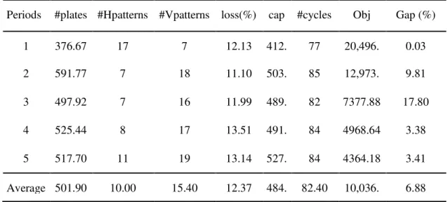
The Tables 2 and 3 show the results of the two instances (MCP_V and MCP_H) considering only the decisions associated to the cutting stock problem: the total number of plates (#plates), the number of cutting patterns (#Hpatterns – for Homogeneous), (#Vpatterns – for Plant V) and (#HTCpatterns – for Heuristic HTC), the material average losses (loss (%)), the usage of the cutting machine capacity (cap), the number of cutting machine cycles (#cycles). The tables also show the overall costs computed according to the objective function (1) (obj) and the associated integer gap (gap (%)). The integer gap is computed as

(

LSLI_LS

)

*

100

_{, where}_LS_and_LI_{are the values of the best integer solution and the best}

lower bound obtained by the Xpress solver within the time limit of one hour.

The objective of the comparison between the results presented in Table 2 and Table 3 was to evaluate the influence of the cutting patterns in the model solution. The conclusions we get from the comparison are that the instance MCP_V uses less homogeneous cutting pattern and the losses are smaller, but the number of plates is higher. The number of cutting machine cycles is equivalent in both instances. It is worth to remember that the instance MCP_V has a total of 122 different cutting patterns against 87 from the instance MCP_H what allows better combinations for instance MCP_V.

Table 2: Solution of instance MCP_V

Periods #plates #Hpatterns #Vpatterns loss(%) cap #cycles Obj Gap (%)

1 376.67 17 7 12.13 412. 77 20,496. 0.03

2 591.77 7 18 11.10 503. 85 12,973. 9.81

3 497.92 7 16 11.99 489. 82 7377.88 17.80

4 525.44 8 17 13.51 491. 84 4968.64 3.38

5 517.70 11 19 13.14 527. 84 4364.18 3.41

(12)

Table 3: Solution of instance MCP_H

Periods

#plates #Hpatterns #HTCpatterns loss(%) cap #cycles Obj Gap (%)

1 454.64 19 6 15.10 503 85 20,691. 0.81

2 494.75 23 10 17.08 522 84 10,989. 15.22

3 461.48 21 10 16.67 520 84 5770.50 6.92

4 486.77 22 9 16.57 507 83 4671.23 3.74

5 447.56 20 11 16.33 441 77 4301.90 0.19

Average 469.04 21 9.2 16.35 498 82.60 9284.93 5.37

Observe that the average objective value (obj) over the five periods given in instance MCP_H is 7,48% smaller than the one given in instance MCP_V what shows that the instance MCP_H has better results for the combined problem: lot sizing and cutting machine. Further, observe that for two days (day 1 and 5) the gap(%) is less than 1% which means that it is very close to the optimum solution. In the next section the lot sizing results are evaluated in detail.

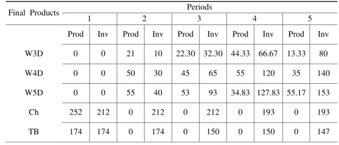
3.2 Lot Sizing Results

The Tables 4 and 5 show the results of the two instances (MCP_V and MCP_H) considering only the decisions associated to the lot sizing problem. The first column of each period shows the production (Prod) and the second column shows the inventory (Inv) of final products.

Table 4: Production and inventory of the final products in each period given by solution of instance MCP_V

Final Products Periods

1 2 3 4 5

Prod Inv Prod Inv Prod Inv Prod Inv Prod Inv

W3D 0 0 21 10 0 10 70 70 10 80

W4D 0 0 50 30 45 65 20.8 85.8 54.3 125.1

W5D 0 0 33.8 18.8 55 73.8 29.2 103 36.95 109.9 5

Ch 290 250 0 250 0 250 0 231 0 231

TB 174 174 0 174 0 150 0 150 0 147

(13)

level for final products in each period (see Table 1), the solution of instance MCP_ H is slightly better than the solution of instance MCP_V. The instance MCP_H maintains the inventory for final products above the minimum level for all products and periods but for the products of the Group 1 in the first period and for the final product W4D in the second period. It also maintains, in general, the inventory for final products closer to the maximum level.

Table 5: Production and inventory of the final products in each period given by solution of instance MCP_H

1 2 3 4 5

Prod Inv Prod Inv Prod Inv Prod Inv Prod Inv

W3D 0 0 21 10 22.30 32.30 44.33 66.67 13.33 80

W4D 0 0 50 30 45 65 55 120 35 140

W5D 0 0 55 40 53 93 34.83 127.83 55.17 153

Ch 252 212 0 212 0 212 0 193 0 193

TB 174 174 0 174 0 150 0 150 0 147

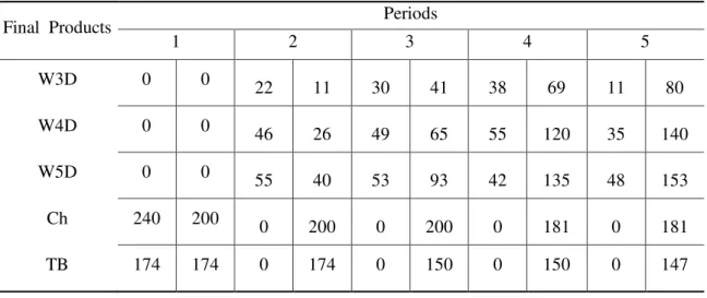
3.3 Results for the strategy to reduce the number of cutting machine cycles

The number of cutting machine cycles can be reduced when constraints (19) are included in the model replacing constraints (13). The results obtained with this new strategy (MCP_H1) are shown in Tables 6 and 7.

Table 6: Solution given by strategy MCP_H1

Periods #plates #Hpatterns #HTCpatterns loss(%) cap #cycles Obj Gap (%)

1 478.56 21 5 14.15 47 83 20,749. 1.09

2 544.83 24 7 14.14 49 82 11,346. 16.41

3 498.44 20 10 16.64 52 84 5722.86 6.18

4 489.38 23 8 18.22 52 82 4657.09 3.76

5 473.56 14 14 14.17 42 76 4360.98 0.17

Average 496.96 20.40 8.80 15.46 48 81.40 9367.39 5.52

(14)

solution of strategy MCP_H and the production of final products is almost the same in all periods (Tables 4 and 7), this means that there is a higher number of pieces in stock.

It is interesting to notice that a smaller number of cutting patterns does not always imply a reduction in the number of cycles. For example, in period 1 the solution given in MCP_H uses 25 cutting patterns and 85 cycles while the solution of MCP_H1 uses 26 patterns and 83 cycles. This has already been noted in other studies to reduce the number of cutting machine cycles (Mosquera and Rangel (2007)). For papers that deal with the reduction of the number of different cutting patterns see Yanasse and Limeira (2006) and Alves and Valerio de Carvalho (2008).

Table 7: Production and inventory of the final products in each period given by solution of strategy MCP_H1

1 2 3 4 5

W3D 0 0 ₂₂ ₁₁ ₃₀ ₄₁ ₃₈ ₆₉ ₁₁ ₈₀

W4D 0 0 ₄₆ ₂₆ ₄₉ ₆₅ ₅₅ ₁₂₀ ₃₅ ₁₄₀

W5D 0 0 ₅₅ ₄₀ ₅₃ ₉₃ ₄₂ ₁₃₅ ₄₈ ₁₅₃

Ch 240 200 ₀ ₂₀₀ ₀ ₂₀₀ ₀ ₁₈₁ ₀ ₁₈₁

TB 174 174 0 174 0 150 0 150 0 147

4 Conclusions

In this paper the furniture industry production process is studied. A new mixed-integer optimization model is proposed combining the lot sizing and cutting stock decisions on a rolling horizon basis. The model considers operational decisions related to the cutting machine programming problem taking into account the decisions related to lot sizing problem. The combined model was tested with a set of data obtained from a small-size furniture factory. The computational tests highlight some areas of the production planning directions that can be improved by considering a small number of cutting patterns and including a strategy to improve the machine utilization.

A drawback of the solution approach is that the cutting patterns used in the model are generated a priori. A column generation approach, for generating the cutting patterns, might help to improve the solution quality and reduce the computational time. This is an interesting topic for future research.

To the best our knowledge the combined model proposed in this paper is the first one to take into account operational decisions related to the cutting machine programming (saw cycle and setup decisions) when planning the cutting patterns and the lot sizing. Therefore a comparison with other combined models of the literature was not possible.

(15)

Ongoing efforts are continuing with the furniture factory to obtain the data necessary for a more precise comparison between the decisions currently used in practice and those output by the proposed model. In parallel, other furniture factories in the region are being sought for further case comparisons. To facilitate such collaboration, a tool with a visual interface needs to be developed, within a wider objective of providing production planning and scheduling software for small and medium-sized furniture factories.

Acknowledgement - The authors would like to thank the referees for the valuable reviews and helpful suggestions. This work was partially funded by the Brazilian agencies FAPESP, CNPq and CAPES, and the FP7-PEOPLE-2009-IRES Project (no. 246881).

References

Alves, C.; Valério de Carvalho, J. M. (2008) A branch-and-price-and-cut algorithm for the pattern minimization problem. RAIRO Operations Research, v.42, p. 435-453.

Araujo, S. A., Rangel, S. and Santos, S. G. (2008a) Lot Sizing and Cutting Machine Programming Problem in Furniture Industry. 4th International Conference on Production Research - ICPR Americas’ 2008.

Araujo, S. A., Arenales, M. N. and Clark, A. R. (2008b). Lot-Sizing and Furnace Scheduling in Small Foundries, Computers and Operations Research, 35, 916 – 932.

Araujo, S. A., Arenales, M. N. and Clark, A. R. (2007). Joint Rolling-Horizon Scheduling of Materials Processing and Lot-Sizing with Sequence-Dependent Setups, Journal of Heuristics, 13, 337 – 358. Arbib, C. and Marinelli, F. (2005). Integrating process optimization and inventory planning in

cutting-stock with skiving option: an optimization model and its application. European Journal of Operational Research 163 (3), 617 – 30.

Carnieri, C, Guillermo, A and Gacinho, L (1994). Solution procedures for cutting lumber into furniture parts. European Journal of Operational Research, 73, 495 – 501.

Cavichia, M. and Arenales, M. (2000). Piecewise linear programming via interior points, Computers & Operations Research, 27, 1303 – 1324.

Clark, A. R. (2003). Optimization Approximations for Capacity Constrained Material Requirements Planning Problems, International Journal of Production Economics, 84, 115 – 131.

Clark, A. R. (2005). Rolling Horizon Heuristics for Production and Setup Planning with Backlogs and Error-Prone Demand Forecasts, Production Planning and Control, 16, 81 – 97.

Dash-Optimization (2009). Modeling with Xpress-mp. (available in: www.dashoptimization.com -last visit: 28/10/2009).

Drexl, A. and Kimms, A. (1997). Lot Sizing and Scheduling - Survey and Extensions, European Journal of Operational Research, 99, 221 – 235.

Farley, A. (1988). Mathematical programming models for cutting-stock problems in the clothing industry, Journal of Operations Research Society, 1, 41 – 53.

Fleischmann, B. and Meyr, H. (1997). The General Lotsizing and Scheduling Problem, Operational Research Spektrum, 19, 11 – 21.

(16)

Gramani, M., França, P. M. and Arenales, M. N. (2009). A Lagrangian relaxation approach to a coupled lot-sizing and cutting stock problem, International Journal of Production Economics, 119, 219 – 227. Haessler, R. W. (1971). A heuristic programming solution to a nonlinear cutting stock problem.

Management Science, 17 (12), 793-812.

Hendry, L., Fok, K. and Shek K. (1996). A cutting stock and scheduling problem in a copper industry, Journal of Operations Research Society, 47, 38 – 47.

Landi, F.R. and Gusmão, R. (2005). Indicadores de ciência, tecnologia e inovação em São Paulo 2004, FAPESP, São Paulo, V 1. (available in www.fapesp.br/indicadores - last visited march/2006)

Morabito, R and Arenales, M (2000). Optimizing the cutting of stock plates in a furniture company. International Journal of Production Research, 38, 2725 – 2742.

Mosquera, G. P. and Rangel, S. (2007). Redução de ciclos da serra no problema de corte de estoque bidimensional na indústria de móveis. In: XXX CNMAC, 2007, Florianópolis. XXX CNMAC - Trabalhos e Resumos - CD ROM. São Carlos - SP: SBMAC.

Nonas, S. and Thorstenson, A. (2000) A combined cutting-stock and lot-sizing problem, European Journal of Operational Research, 120, 327 – 342.

Nonas, S. and Thorstenson, A. (2008). Solving a combined cutting-stock and lot-sizing problem with a column generating procedure, Computers & Operations Research 35, 3371 – 3392.

Poltronieri S., Poldi K., Toledo F., Arenales M. (2007) A coupling cutting stock-lot sizing problem in the paper industry, Annals of Operations Research, 157, 91-104.

Rangel, S. and Figueiredo, A. (2006). Generation of productive 2D-cutting patterns for the furniture industry. In: Anales del XIII Congreso Latino-Iberoamericano de Investigación Operativa, v. único. p. T120.

Rangel, S. and Figueiredo, A. (2008). O problema de corte de estoque em indústrias de móveis de pequeno e médio portes. Pesquisa Operacional, 28, 3, 451-472.

Respicio, A. and Captivo M. (2002). Integrating the cutting stock problem in a capacity panning, Department of Informatics and Centre of Operational Research, University of Lisbon, Portugal.

Silva C., Alem D., M. Arenales A. (2007). Combined cutting stock and lot-sizing problem in the small furniture industry. In: Anais do XXXIX Simpósio Brasileiro de Pesquisa Operacional.

Silva, E. (2003). Alinhamento das Estratégias competitivas com as estratégias de produção: Estudo de casos no Pólo Moveleiro de Votuporanga/SP, Dissertação, Pós-Graduação em Engenharia de Produção, USP, São Carlos, Brazil.

Stadtler, H. (2003). Multilevel Lot Sizing with Setup Times and Multiple Constrained Resources: Internally Rolling Schedules with Lot-Sizing Windows, Operations Research, 51, 487 – 502.

Stipp, M. (2002). Cluster Industrial: O Pólo moveleiro de Votuporanga-SP (1962-2001), Dissertação de Mestrado, FCL - UNESP, Campus de Araraquara, SP, Brazil.

Suerie, C. and Stadtler H. (2003). The Capacitated Lot-Sizing Problem with Linked Lot-Sizes, Management Science, 49, 1039 – 1054.

Suzigan, W. (2000) Industrial Clustering in the state of Sao Paulo, working paper CBS-13-00(E), University of Oxford Centre for Brazilian Studies, Oxford, U.K..

Valença, A., Pamplona, L. and Souto S. (2002). Os novos desafios para a indústria moveleira no Brasil, BNDES Setorial, 15, 83 – 96.

(17)

Yanasse, H., Harris, R. and Zinober A. (1993). Uma heurística para redução do número de ciclos da serra no corte de chapas, Anais do XIII ENEGEP / Congresso Latino Americano de Engenharia Industrial, 879 – 885.