The effect of anthropogenic noise as a source of acoustic stress in wild populations of Hippocampus guttulatus in the Ria Formosa

Marisa Raquel Gonçalves Magalhães

The effect of anthropogenic noise as a source of

acoustic stress in wild populations of Hippocampus

guttulatus in the Ria Formosa

U

NIVERSIDADE DO

A

LGARVE

FACULDADE DE CIÊNCIAS E TECNOLOGIAS

T

ESE DE

M

ESTRADO DE

B

IOLOGIA

M

ARINHA

Faro, Setembro 2016

The effect of anthropogenic noise as a source of acoustic

stress in wild populations of Hippocampus guttulatus in the

Ria Formosa

Master Thesis of Marine Biology

Dissertation supervised by Doctor Jorge Palma (CCMAR)

U

NIVERSIDADE DO

A

LGARVE

FACULDADE DE CIÊNCIAS E TECNOLOGIAS

T

ESE DE

M

ESTRADO DE

B

IOLOGIA

M

ARINHA

The content of this work is the sole responsibility of the author

Declaro ser a autora deste trabalho, que é original e inédito. Autores e trabalhos consultados estão devidamente citados no texto e constam da listagem de referências incluída

Assinado:

(Marisa Raquel Gonçalves Magalhães)

Faro

UAlg©_{A Universidade do Algarve reserva para si o direito, em conformidade com o disposto no} Código do Direito de Autor e dos Direitos Conexos, de arquivar, reproduzir e publicar a obra, independentemente do meio utilizado, bem como de a divulgar através de repositórios científicos e de admitir a sua cópia e distribuição para fins meramente educacionais ou de investigação e não comerciais, conquanto seja dado o devido crédito ao autor e editor respectivos”.

A

To CCMAR and to the people that work at Ramalhete, that contributed through the

first 2 months of my thesis, to my knowledge about seahorses and seahorse’ aquarium

maintenance techniques and feeding habits.

To Doctor Jorge Palma for having accepted to guide me, and allowing my constant learning about seahorses, both in captivity and in the wild, for all the dives and for the support and encouragement always demonstrated, as well as the willingness and commitment to my work.

To Doctor Miguel Correia from CCMAR for assisting in the field work, for having provided his previous studies and for being helpful whenever needed.

To Cristiano Soares from Marsensing® for all the help in the section of sound analysis of my work and all the explanations of the material’ functioning and operation.

To professor Paulo Relvas for his help to clarify some of my doubts about physics oceanography and sound propagation on water.

To my family and friends for the unconditional support. A special thanks to my parents and all my family that helped me through all these years financially and emotionally, being far away from home, just to help me achieve my goals and dreams since I can remember.

To my boyfriend and friend Luis for the patience and love, for all the coffees and

encouragement’ war cries shouted from the living room and specially for keeping my

R

Os cavalos-marinhos são peixes de pequenas dimensões com uma morfologia particular (rápido crescimento, maturação precoce e tempos de geração curtos) que utilizam a sua cauda preênsil para se manterem agarrados a estruturas sésseis. Possuem elevada fidelidade a habitats preferenciais e baixa fecundidade. Devido á sua biologia e ecologia específicas, os cavalos-marinhos ocorrem principalmente em zonas costeiras de baixa profundidade, onde em muitos casos, o impacto antropogénico implica uma crescente degradação ambiental à qual estas espécies têm dificuldade em fazer face. Dada a sua sensibilidade às alterações de habitat, são consideradas espécies bandeira (flagship species) e por isso, representativas do habitat onde se incluem (e de outras espécies com quem o partilham), pelo que o seu estudo é de vital importância na salvaguarda da biodiversidade marinha. Cavalos-marinhos da espécie Hippocampus guttulatus são conhecidos por co-existir, juntamente com Hippocampus hipocampus na Ria Formosa, mas a partir de 2000 até agora, verificou-se uma grande redução de sua sustentabilidade na Ria, com uma redução na lagoa de 73% e 94% para o H. hipocampus e H. guttulatus, respectivamente, em menos de 10 anos. São vários os impactos antropogénicos que se julga poderem causar de forma directa ou indirecta, alterações no ecossistema da Ria Formosa, nos quais se incluem factores como a eutrofização, poluição, dragagens, captura acessória por artes de pesca (by-catch), destruição das pradarias marinhas e dos habitats preferenciais e poluição sonora aquática. Quando expostos a situações de poluição sonora subaquática, os cavalos-marinhos podem evidenciar respostas de stress que condicionam o seu bem-estar, incluindo, diminuição do crescimento, perda auditiva e complicações no processo reprodutivo. Estudos semelhantes em peixes e camarões apontam para taxas de crescimento mais lentas, taxa de mortalidade mais elevada, menor ingestão de alimentos, taxas de canibalismo mais elevadas, doenças, taxa de reprodução diminuída, consumos mais elevados de O2e elevado número de excreções de NH3. No entanto, a maior parte

destas conclusões resultam de estudos efectuados em cativeiro, sendo o presente um dos primeiros a ser realizado em condições naturais, e o primeiro na Ria Formosa. Neste estudo, espécimes de cavalo-marinho-de-focinho-comprido, Hippocampus guttulatus foram expostos a diferentes condições acústicas de forma a poder identificar quaisquer reacções fisiológicas a esse estímulo. Para tal, testaram-se dois tipos de som: de motor de barco em trânsito (entre 63.4 e 127.6dB) e desse mesmo motor em situação estática e

contínua (até 137.1dB). Durante um período de três minutos (2 minutos para som transitório e 1 minuto para som constante) e utilizando um conjunto de câmara de vídeo e hidrofone, recolheu-se informação de 60 indivíduos (49 observações válidas: 46 H.

guttulatus (29 machos e 17 fêmeas) e 3 H. hippocampus (2 machos e uma fêmea))

observados entre os 4 e os 10 metros de profundidade em dois locais de amostragem. Foram observadas, de facto, mudanças comportamentais pela parte dos cavalos, observou-se um aumento significativo (p<0.05) na taxa de respiração, facto que se verificou em 87.8% dos animais observados. O número de batimentos operculares por minuto (OMPM) dos cavalos-marinhos da espécie H. guttulatus aumentou de 35,7±10 (amostra no controlo) para 41,2±15,5 no primeiro minuto de observação, para 45,5±13,3 no segundo (ambos sob som em trânsito) e para 49,7±12,5 no terceiro minuto (sob exposição a som constante). Observaram-se igualmente, diferenças significativas entre os valores médios de OMPM dos peixes da amostra controlo e os observados durante o segundo minuto (p<0.01) e durante o terceiro minuto (p<0.0001) e um aumento significativo (p<0.05) nos OMPM de peixes observados durante o primeiro e o terceiro minuto. Para além disso, 30.6% dos peixes ficaram mais irrequietos e/ou abandonaram o local de observação numa tentativa de evitar o estímulo sonoro negativo. Observações de cavalos-marinhos no selvagem em condições de tráfego normal foram também realizadas num terceiro local de amostragem segundo os mesmos parâmetros, apenas com a ausência de som provocado. Após as observações, os vídeos foram analisados de maneira a quantificar os movimentos operculares, movimentos esses que foram posteriormente comparados às observações feitas no controlo. De 35,7±10 movimentos operculares por minuto observados no controlo para 45.6±10.1 dos animais no selvagem em condições de tráfico normal, foi verificado um aumento significativo (p<0.05) de 9.9 movimentos operculares por minuto (27.7%). Uma diferença na respiração entre machos e fêmeas foi também notada, com diferenças de 35.5±14.1 movimentos operculares por minuto nos machos para 44.3±15.4 nas fêmeas no primeiro minuto das passagens do barco, de 37.8±13.1 nas fêmeas para 49.2±13.1 nos machos no segundo minuto (ambas de som transitório) e finalmente de 45.3±12.3 nas fêmeas para 53.1±14.1 nos machos no terceiro minuto das observações correspondente ao som estático contante. Essas diferenças mostraram ser não significativas (p>0.05) e foram também observadas num ambiente controlado com uma diferença em média de 29.8±9.8 movimentos operculares por minuto das fêmeas para 39.9±9.7 movimentos operculares dos machos, também elas não significativas (p>0.05).

Registos sonoros foram também analisados utilizando o programa Audacity® para verificar diferenças ao nível de som perceptível entre o som produzido pelas transições do barco com o som constante e mesmo dentro das transições, quando o barco se encontrava mais afastado da bóia (lançada quando um animal era encontrado, indicando ao skipper para iniciar as transições) e de quando se encontrava mais perto. Médias de dB foram quantificadas e valores máximos e mínimos de médias (e de valores dentro de médias) foram quantificados para posterior elaboração de análises de frequência. Com base no observado, os resultados apontam para um claro impacto do barulho subaquático causado por fontes antropogénicas sob as populações selvagens de H. guttulatus na Ria Formosa. O presente plano de trabalho pretende avaliar este último factor e verificar se o ruído aquático de origem antropogénica, causado nomeadamente por motores de embarcações de diferente potência e calado constitui uma fonte de stress acústico para as populações selvagens de H. guttulatus, indutora de comportamentos atípicos para a espécie e que possa de alguma forma ter um impacto negativo na sua qualidade de vida. Se relevante, os resultados irão ser usados como ferramenta de gestão para prevenir este tipo de perturbação em áreas onde a espécie ainda ocorre em números significativos.

Palavras-chave: H. guttulatus, cavalo-marinho, comportamento, stress acústico,

A

When exposed to underwater noise disturbances, seahorses are reported to display stress responses that affect their life-history, including slower growth, hear loss and reproductive impairment. Prior to this study, most of these conclusions were inferred from experiments held in captivity. The present study, was one of the first to be performed in natural conditions and the first in the Ria Formosa. In this experiment, long snout seahorse, Hippocampus guttulatus specimens were exposed to potential acoustic stress factors in order to evaluate eventual physiological stress responses. Two different underwater noises with different sound intensities were tested: transient motor boat sound (63.4dB to 127.6dB) and constant sound produced by the motor boat anchored directly above the animals, up to 137.1 dB. A total of 60 fish (49 valid observations) were observed between 4 and 10 meters depth throughout a three minute period using a video camera and a hydrophone set. A significant increase (p<0.05) in the respiratory rate was observed in 87.8% of the observed fish. Opercular movements per minute (OMPM) increased from 35,7±10 (control sample) to 41,2±15,5 in the first minute of observations, to 45,5±13,3 in the second (both under transient sound) and to 49,7±12,5 in the third (under constant sound exposure). Significant differences in means between the control fish and fish observed during the second (p<0.01) and third minute of observation (p<0.0001) were observed. Concordantly, a significant increase (p<0.05) in the OMPM of fish observed in the 1st minute and the 3rd minute was noted. In addition to the OMPM increase, 30.6% of the animals abandoned the observation location in an attempt to avoid the negative sound stimuli. Based on the obtained information, results showed a clear impact of underwater anthropogenic noise as a negative stress factor for the wild populations of H. guttulatus in the Ria Formosa lagoon.

T

O

C

Table of Contents ……….………....…... vii

List of tables……….……….………... viii

List of figures……….………... ix

1. Introduction……….………... 1

2. Study Area………..…..……. 5

3. Material and Methods………..…………..….. 7

3.1 Species description………..……….... 7

3.2 Sound and video recording in the natural environment – in situ experiments …… 9

3.3 Controlled environment - ex situ: measurements for control …………..……….. 11

3.4 H. guttulatus Observations in the wild ………..……....… 12

3.5 Working with software Audacity ……….……….….... 13

3.6 Statistical Analysis ………..…….….… 16

4. Results ……….….… 17

4.1. Video Analysis………..… 17

4.1.1. Natural environment - in situ experiments ……….….. 17

4.1.2. Observations in the wild (normal boat traffic) …….……….….. 20

4.2. Hydrophone Analysis ……….…. 21

4.2.1. Male vs Female respiratory’ rate per dB ………... 25

4.2.2 dB per depth ………...……….. 27

5. Discussion ………..….. 31

6. Conclusions ………. 41

L

O

T

Table 4.1: Observed average (average±s.d.), minimum and maximum number of OMPM in H.

guttulatus and H. hippocampus ………..…19

Table 4.2: Statistics descriptive of Tukey´s multiple comparisons test between H. guttulatus

OMPM control values and data obtained under natural conditions

………....… 19 Table 4.3: Observed average (average±s.d.), maximum and minimum number of OMPM in

H. guttulatus ……….…… 20

Table 4.4: Significant differences in OMPM means between control and animals in the wild……….... 20 Table 4.5: Average (average±s.d.), minimum and maximum sound exposure (in dB) of H.

guttulatus observed under natural traffic conditions……… 24

Table 4.6: No significant differences in OMPM means between males and females on control

and observations animals in the wild …………...………... 26

Table 4.7: Number of observed animals per depth class ………....… 27 Table 4.8: OMPM (opercular movements per minute) and dB per each observation depth class

between 4 and 10 meters ………. 27

L

O

F

Figure 1.1: External morphology of a seahorse: whole lateral view (top left), trunk rings (top

right) and head dorsal (bottom left side) and lateral (bottom right side) side view (adapted from Lourie et al., 2004) ………...…………... 1

Figure 3.1: H. guttulatus morphology (adapted from Lourie et al., 2004) ………....… 7 Figure 3.2: H. guttulatus color (Illustrator – Jorge Palma) ……….………...… 8 Figure 3.3: Hydrophone and video camera apparatus (1-Camera, 2- Hydrophone,

3-Weight)……….. 10

Figure 3.4: Ria Formosa sampling site location; virtual image from Google Earth …..…… 11 Figure 3.5 and 3.6: H. guttulatus and H. hippocampus broodstock tanks at Ramalhete experiment

filed station ……… 12

Figure 3.7: dB scale from 1 to zero ………...………….…… 14 Figure 3.8: Soundwaves: Difference between transient sound (top left) and transient sound with

zoom (top right) and recurrent sound (bottom left) and recurrent sound with zoom (bottom right) using Audacity. Left images: peak levels in dark blue and root mean signal (RMS) average loudness in light blue ……….... 15

Figure 3.9: Clipping in Audacity ………... 15 Figure 4.1: Observed behavior response of H. guttulatus when exposed to boat sound…….... 17 Figure 4.2: Respiration rate: Opercular movements per minute during control vs experiment

during the 1st_{, 2}nd_{and 3}rd_{minute ………...… 18}

Figure 4.3: Opercular movements per minute during control vs observations in the wild ..… 21 Figure 4.4: Spectrogram of transient sound of boat passages (top) and constant sound (bottom),

1- Loud sound in red (from boat approximation); 2- Quiet sound in blue (from boat departure)

……….……... 22 Figure 4.5: Example of frequency analysis during boat transitions with the boat departed from

the buoy ………. 23

Figure 4.6: Example of frequency analysis during boat transitions with the boat near the buoy

... 23

Figure 4.7: Example of frequency analysis during constant sound with the boat near the buoy ……….….. 24 Figure 4.8: Comparison between the number of OMPM and respective dB exposure of male and

female H. guttulatus during the observation period ………..… 25

Figure 4.9: Comparison of the number of OMPM between male and female H. guttulatus during

control, observations in the wild and during sound trials ………..………….…... 25

Figure 4.10: Comparison of the number of OMPM and standard deviation between male and

Figure 4.11: OMPM and dBs per depth during the first minute of observation under natural

conditions ……….. 29

Figure 4.12: OMPM and dBs per depth during the second minute of observation under natural

conditions ………... 29

Figure 4.13: OMPM and dBs per depth during the third minute of observation under natural

conditions ………... 30

Figure 4.14: Decibels (dB) default values (constant sound) per depth………... 30 Figure 5.1: Comparison of densities of H. guttulatus during underwater visual census surveys in

2001/2002 (Curtis and Vincent, 2005) and 2008/2009 (Caldwell, 2012) in the Ria Formosa lagoon (adapted from Caldwell, 2012 PhD thesis) ………..…. 32

1. I

Seahorses (Hippocampus) belong to the Syngnathidae family along with pipefishes and seadragons.The name originate from the greek, means fused ‘syn’ and jaws ‘gnathus’ and relates to the tube-snout present in all Hippocampus species (Ahnesjö et al., 2011).

The flexible and fracture resistant body armor of seahorses (Figure 1.1) consists in plates and segments (designed to slip and slide when compressed) which overlay to allow a ventral curving (Vecchione, 2014) and in addition to their peculiar morphology, their prehensile tail is used to hold onto different holdfasts, from coral to sponges, mangroves, seaweeds and even artificial structures (Correia et al., 2015).

(Figure 1.1): External morphology of a seahorse: whole lateral view (top left), trunk rings (top right) and head dorsal (bottom

left side) and lateral (bottom right side) side view (adapted from Lourie, S., A., et al. 2004).

Among Syngnathids, there are many socially and genetically monogamous species that mature clusters of eggs in synchrony particular among seahorses whereas many other species are polygamous or polyandrous producing eggs in asynchrony continuously or in small batches (Ahnesjö et al. 2011).

A unique interesting singularity of the Syngnathidae is male pregnancy. For a long time, pouch bearing of seahorse embryos was assigned to the female and the first male

“false belly” was published by Ekstörm in 1831 (Stölting & Wilson, 2007). Seahorses

have low fecundity but they developed an extreme parental care where the embryos

develop in the male’s pouch (marsupium) where they are kept protected in an oxygenated

and osmotically regulated environment (Jesus, 2011). When juveniles leave the male’s pouch, they are smaller but very similar to the adult seahorses, feeding immediately on live prey (Vecchione, 2014) ceasing from that point on any further parental care. Juveniles may then spend a minimum of 8 weeks pelagically drifting before recruiting to benthic habitats (Curtis & Vincent, 2004) with the possibility of being targeted by other fish, resulting in high mortality rates (Vecchione, 2014).

Seahorses mature at about four to twelve months depending on the species and their lifespan range from about one year in the smaller species to about three to five years in the larger species (Lourie et al., 2004). Predation is higher on juveniles, which are eaten by fish and invertebrates while adult seahorses are presumed to have few predators due to an excellent camouflage effect and a presence of a not so savory bony plates and spines (Lourie et al., 2004).

Throughout their life stages, seahorses feed mainly on crustaceans, mostly on copepods during the early stages and later on small shrimp, mysid shrimp, amphipods, and even larval fish (Kitsos et al., 2008). Seahorse hatch already with a fully developed digestive system composed by a simple digestive apparatus, with a buccopharynx, oesophagus, an intestine (composed of a midgut with intestinal villi) and a hindgut preluded by and intestinal valve (Palma et al., 2014; Vecchione, 2014).

The maximum reported depth for H. gutullatus in particular is 12 meters, inhabiting shallow inshore waters in seaweeds and algal stands and during winter, deeper depths and rocky areas (Lourie et al., 2004). They are (mostly) cryptic fishes with slow movements, remaining static throughout long periods of time which, if by one side make them fit for ecological studies in the field, in the other, difficult their detection, identification and survey (Ahnesjö et al., 2011). Most seahorse species use their prehensile tail as a means to grasp different holdfasts, from sponges to coral, shells, macroalgae, benthic invertebrates, seagrass, mangrove branches and even artificial structures thus relying on some degree of habitat structure (Lourie et al., 2004; Foster & Vincent, 2004).

Unlike H. hippocampus that are known to be habitat generalists which helps them to cope with natural variability and unpredictable changes due to habitat degradation or

even habitat loss (Owens & Bennett, 2000; Harcourt et al., 2002; Krauss et al., 2003; Cunha et al., 2011; ; in Caldwell, 2012), H. guttulatus rather appreciate more complex habitats relying on site fidelity. This means that this species face an increasing difficulty in adapting or tolerating changes and environmental impacts if they occur. This constitutes a problem since these areas that they inhabit are in many cases subjected to anthropogenic impacts, implying an increasing environmental degradation to which these species have a coping deficiency (J. Palma pers. comment).

Seahorses contribute to marine biodiversity and to the function of the ecosystem and in order to access the effects of incidental catch and to promote management conservation strategies and to secure their persistence in the wild it is important to better understand their population parameters and life history (Foster & Vincent, 2004). In the

International Union for Conservation of Nature’s (IUCN) Red List assessment it is held

that for the 41 species of existing seahorses, 27 are given the status of Data deficient (including H. hippocampus and H. guttulatus), 11 as Vulnerable, 1 Endangered, 1 Near Threatened and 1 as Least concern (IUCN, 2016).

Understanding seahorse life history is also of major importance since the entire

Hippocampus genus was added to Appendix II of the Convention of International Trade

in Endangered Species of Wild Fauna and Flora (CITES) providing traffic regulations for those species (Correia, 2014). Species listed in Appendix II like H. guttulatus are those where the wild populations are or may become threatened by international trade. It’s a way to try to safeguard that future use of these species is taken in a sustainable manner where trade is allowed but with exporting parties having to ensure that their exports do not damage and are not harmful to wild populations (Lourie et al., 2004).

Thus, given their data-deficient status and their sensibility to habitat changes, they are considered flagship species, therefore representative of the habitat they comprise and the animals that cohabit with them, whereby their study is of vital importance for the conservation of marine biodiversity. Shokri et al. (2009) showed that syngnathids could be used as an efficient flagship group to select MPAs for other fish in one estuarine system, being a species that attract public support and sympathy and therefore can possibly attract funding for protection (Caro & O’Doherty, 1999; Andelman & Fagan, 2000). By focusing on conservation needs of one flagship species, other less charismatic taxa may be protected simultaneously (Caro & O’Doherty, 1999) and consequently being possible that conservation planning directed at syngnathids may have coincidental benefits for many other species of fish that also inhabit seagrass beds (Shokri et al., 2009).

Seagrass beds are preferred by juveniles and adults of many species of fish since they provide a nursery habitat for early life stages of fish (Pollard, 1984; Bell & Pollard, 1989; Hindell et al., 2000). Since shallow coastal areas, preferred by seahorses, are where anthropogenic disturbances tend to be more frequent and severe (Bell et al., 2003) and again, given their low fecundity, parental care, site fidelity, limited distribution and sedentary nature (low mobility), syngnathids are considered to be highly vulnerable to human impact (Foster & Vincent, 2004).

H. guttulatus are known to co-exist along with H. hippocampus in the Ria Formosa

but from 2000 until now, it was verified a major reduction of their sustainability in the Ria, with a reduction within the lagoon of 73% and 94% for of H. hippocampus and H.

guttulatus respectively in less than 10 years (Caldwell & Vincent 2012; Correia, 2014).

Many human related activities occur in the habitats that are preferred by seahorses, such as, aquatic sports and boat traffic including boat anchoring. These activities increase the environmental disturbance and therefore contribute to the negative pressure on the existing seahorse populations (J. Palma pers. comment).

Underwater sounds produced by all these activities may generate a higher stress factor for these populations since it was verified in other studies that acoustic stress in indeed a factor of disturbance in other marine species. Hastings et al., (1996) noted that underwater sounds equal or greater to 180 dB at 50-2000 Hz would be harmful to fishes and Gisiner et al. (1998) observed physiological effects of intense sound on marine fishes including swim bladder injuries, eye hemorrhages, lower egg viability and growth rates at peak sound pressure levels of 220 dB.

Previous observations in the Ria Formosa (Project HIPPOSAFE, FCT funded) suggest the same problem, with the H. guttulatus populations being effected by boat traffic noise. Therefore, this study aimed to determine the effect of underwater anthropogenic noise caused by boat traffic as a source of acoustic stress in wild populations of H. guttulatus in the Ria Formosa lagoon and an effective cause of disruptive behaviors of this species endorsing negative impacts on their life quality.

2. S

A

This study was conducted in the Ria Formosa lagoon, southern Portugal (36º59’N,

7º51’W), a shallow, estuarine lagoon with 55km long and 6km at its widest point, with

water temperatures ranging seasonally from 12º to 27º (Newton & Mudge, 2003) and connected to the Atlantic Ocean by six inlets. The Ria is an highly productive system with an extensive salt march vegetation, high nutrient concentrations and it is characterized by high water turnover rates and a network of channels and tidal creeks (Curtis & Vincent, 2005).

The western part of the lagoon is heavily urbanized and also used for agricultural purposes. Despite tidal pumping from sediments (Falcão & Vale, 1990) and an exchange with nearby coastal waters (Falcão & Vale, 2003) the Ria as an input of nutrients coming from urban discharges agricultural run-off (Newton & Mudge, 2003) which makes it highly productive and a fitted environment for a lot of different species but also supporting socio economic industries like fishing, tourism, salt extraction and aquaculture which can threaten the species and their habitats.

It is a semi-protected lagoon (it was recognized as Natural Reserve in 1978 and reclassified as a Natural Park in 1987), it forms part of the European network of protected areas Natura 2000 and a protected area of the RAMSAR convention on Wetlands of International importance (Jesus, 2011).

The substrate of the Ria is mostly bare (fine sand, coarse and muddy sand with fragments of shells), with benthic invertebrates and mostly Zostera nolti, Ulva lactuca

and Cymodocea nodosa as the dominant seagrass and macroalgae (pers. observation) and

also the macroalgae Codium spp. (Curtis & Vincent, 2005) as the dominant seagrass and macroalgae.

As it was shown by Caldwell (2012), seahorses were found in the Ria Formosa wrapped around mobile purple sea urchins (Paracentrotus lividus) and this association could accommodate important habitat and protection from predators when another cover is not available. The Ria Formosa lagoon is a highly productive ecosystem and sustains a great variety of commercial species that have high economic value, as among others, the sparid species (Erzini et al., 2002).

South Portugal is a renowned area for tourism and many human related activities occur in the Ria Formosa, including, boat traffic, aquatic sports and boat anchoring. These

activities, combined with the fishing activities by-catch and illegal fishing, over-exploitation for use in commercial trade, curiosities and traditional medicines (Vincent, 1996), increase environmental disturbance and therefore contribute to the negative pressure on the existing seahorse populations. In fact, the use of fishing gears have a direct (by-catch) and indirect (habitat degradation) impact on both seahorse species (Correia, 2014).

3. M

A

M

3.1 Species description

The long-snouted seahorse Hippocampus guttulatus (Cuvier, 1829) is a European species which occurs on the surrounding coasts from the British Isles to the Canary Islands, as well as all of the Mediterranean Sea. According to the SNPRCN (1993) the ecological status of H. guttulatus is undetermined in continental Portugal and rare in the Azores and Madeira Islands. It is a sympatric species along with the short-snouted seahorse, H. hippocampus and one of the only two that exist in the northeast Atlantic including the Ria Formosa (Correia et al., 2015).

Figure 3.2: H. guttulatus color (Illustrator – Jorge Palma).

As it is described by Lourie et al. (2004), the H. guttulatus has a maximum recorded height of 18 cm, it has a total of 11 trunk rings, 35 to 40 tail rings, 17 to 20 dorsal fin rays, 16 to 18 pectoral fin rays and a small but distinct coronet with 5 round knobs or blunt points. It has the coronet not joined smoothly to the neck and a horizontal plate in front of the coronet The spines are medium to well developed with prominent, round eye spines (Figure 3.1) and the color/patter is variable brown with white spots on the body many times with a rink of a dark color around them that tend to blend into horizontal wavy lines (Figure 3.2). It can be mottled or with pale saddles across dorso-lateral surface. 50% of the population reached sexual maturity with 10 cm height and the breeding season extends from March to October. The egg diameter averages 2 mm and gestation lasts 3–5 weeks being the length at birth 12 to 15 mm on average. The offspring’s are planktonic immediately after birth and males have tails proportionally longer than females. In the wild they are found in groups and the maximum reported brood size is 581 (Lourie et al., 2004) being the maximum depth recorded for these animals 12 meters (Caldwell, 2012).

3.2 Sound and video recording in the natural environment - in situ experiments:

In the Ria Formosa lagoon, underwater ambience sound is mainly produced by outboard motor boats, thus one outboard motor boat (5.20 mt long equipped with an 40 hp Yamaha motor) belonging to the Project Seahorse/Fisheries Biology and Hydroecology Group of CCMAR was used. This choice represents the most commonly used combination of boat and outboard motor in the Ria Formosa and can therefore be considered the most important and standard source of underwater noise in this environment.

Sound (including underwater sounds) is normally expressed in dB and its magnitude is in direct relationship with depth, therefore, different depths were covered in this experiment and the recordings of the default sound produced by this boat was collected meter by meter from 1 to 10 meters depth. The sound records were collected using an underwater hydrophone (Marsensing®) in two different circumstances; constant sound and transit or navigation sound.

The transient sound or navigation sound represented the noise produced by a boat in transit passing at a particular location and it was obtained for a set period of time (two minutes) while the constant sound was continuously obtained during one minute, with the boat anchored to try to keep the sound intensity and frequency constant throughout the collection period immediately after the previous recording (transit sound). Additionally, the sound produced by the boat was recorded at different depths (increasing distance to the source) between 4 and 10 meters depth, in order to evaluate any potential depth effect on the seahorse reaction to the stimuli.

Digital hydrophones record the acoustic noise autonomously since they are endowed with memory and they have its own feeding. Some of the relevant technical features of the hydrophone used in this study are:

• Sampling frequency: 50781 samples per second; • Cutting Frequency: 25 kHz.

• Programmable gain of 1, 2, 4, 8, 16, 32, or 64. • Converting analog / digital 16-bit.

• Data Memory: MMC Card 2 Gbyte.

• Autonomy of memory: about 5 hours and 40 minutes (in continuous acquisition).

Besides that, the hydrophone had a programmable amplifier set for a 2x gain and a nominal sensitivity of -162 dB re 1V / 1μPa. The hydrophone was calibrated by recording

test tones from a reference calibrator. The frequency distribution and decibels of chronic (steady state) noise or the peak levels and deviations of acute (transient) noise were measured.

For the video collection it was used a digital camera, Canon G12 with an underwater housing and individual videos were made for each observed fish. Sound and video files were recorded in incorporated memory cards in the two devices and later on downloaded and analyzed with adequate software.

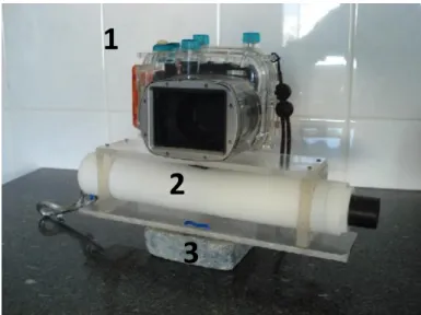
Figure 3.3: Hydrophone and video camera apparatus (1-Camera, 2- Hydrophone, 3-Weight)

For the observations, one scuba diver placed the hydrophone and the video camera (Figure 3.3) close to the seahorse(s), abandoning the location afterword to prevent any kind of interaction/interference with the seahorse in observation. As the hydrophone and camera were placed in position, the diver sent a signal to the surface (by releasing a buoy), alerting the boat skipper to start the boat operation. Each seahorse was observed one single time for a three minute period (two minutes under transit sound and one minute under constant sound) after that, the process was repeated when a new seahorse was found. These recordings were collected during one/two hours’ period during slack high tide, period during which water currents are reduced to a minimum, allowing the diver to operate freely. The number of observations varied from 3 to 25 at each location due to a number of external factors that facilitated or hindered the data sampling (such as visibility, current, tide variation, etc.) and means were reported. During the dives, the seahorse species, sex, depth, temperature and substrate type were recorded.

Later on, collected sound files were analyzed and ranked regarding their characteristics (intensity and frequency) and video files (one per animal) were observed

1

2

3

to detect potential stress responses and to be subsequently compared to the ex situ control sample. Ambient detectable sounds were registered and the sources characterized for later removal during data analysis.

Sample collections were performed in three different locations in the Ria Formosa (site 1 – approx. 36º 59’ 30.55’’N, 7º 53’ 55.96’’ O; site 2 – approx. 36º 59’ 04.56’’ N,

7º 53’ 40.52’’ O and site 3 – approx. 36º59’11.17’’ N, 7º51’42.70’’W (Figure 3.4). Site

selection was based on two important factors, seahorse presence and depth. Site 1 is located in a shallower area, between 4 and 6 meters depth, whereas Site 2 is a deeper area, between 7 to 14 meters depth. Seahorses were observed to the highest depth possible. Site 3 (as being one of the Rias’ location with higher maritime traffic) was chosen to obtain

H. guttulatus observations under normal conditions. Due to the increased human activity

(e. g. boat traffic) recordings were collected during spring and summer time.

Figure 3.4: Ria Formosa sampling site location; virtual image from Google Earth.

3.3 Controlled environment - ex situ: measurements for control

In order to obtain a control sample that could set the values for the basal opercular movements per minute (OMPM), captive born seahorses (both H. guttulatus and H.

hippocampus) reared and maintained in the Aquaculture Research Station of Ramalhete

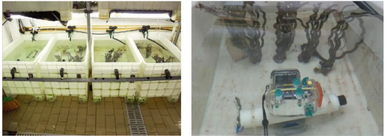
Seahorses are normally kept at a density of 24 fish per tank, in 250 liter plastic tanks assembled in a flow-through system with no sources of distress. The same recording apparatus (video camera plus hydrophone) (Figure 3.3) was gently set in place inside the observation tanks (Figure 3.5 and 3.6) to eliminate any erratic behavior of inherent stress due to its presence. Average temperature and dissolved oxygen in the observation tanks were the same as the recorded under natural conditions.

A total of 16 videos, with an average duration of 3 to 4 minutes each were obtained. The information in them allowed characterizing what is considered a normal, stressed free

H. guttulatus and H. hippocampus breathing situation.

The OMPM were counted to quantify the breathing activity and average breathing per minute both on a gender perspective (male/female OMPM ratio) and overall.

Figure 3.5 and 3.6: H. guttulatus and H. hippocampus broodstock tanks at Ramalhete experiment filed station.

3.4 H. guttulatus: observations in the wild

In order to record the seahorse sound reaction and breathing frequency on site 3, the same procedure and equipment were used. Here, seahorses were observed when exposed to the normal boat traffic in the Olhão channel, one of the more impacted channel in the Ria Formosa. In this situation, the sound occurrence was not controlled, thus matching the fish observation and sound occurrence was random.

A total of 15 videos were recorded between 5.2 to 5.8 meters depth and 15 animals were observed (11 males and 4 females). The same behavior and physiological reactions were analyzed in order to characterize the seahorse breathing under normal boat traffic

conditions (latter on referred as wild). Later on, these values were compared to the previously obtained values.

3.5 Working with software Audacity

The noise associated with boats depends mostly on the type of engine they have. Even small boats can generate large amounts of noise. For example, small boats with large outboard motors can produce sounds on the order of 175 dB re 1 microPa @ 1m. (Conservation and Development’ Problem Solving Team: Graduate Program in Sustainable Development and Conservation Biology, 2009).

The decibel system (dB) is a way to measure sound intensity being intensity perceived as power per area. The low frequency noises that humans can hear are in the order of 10-12wm-2and the loudest in the order of 1wm-2. The region between 10-12wm-2 (essentially zero) and 1wm-2is therefore the audible sound range. dB values are calculated using a logarithmic scale:

dB level = 10 log10I/I0

Where I is the intensity and I0a base intensity (threshold of hearing = 10-12wm-2).

So when the intensity is 1 we have:

10 log10(1/10-12) = 10 log10(1012) = 10*12 = 120 dB level

120 dB can be defined as the “threshold of pain” but saying that humans can hear this dB level with no problem, or if it is high enough to hurt or damage ear canal, that is frequency dependent:

20 Hz ≤ f ≤ 20 000

A frequency lower than 20 Hz it is not audible by the human hear, and only some vibrations are felt and if the frequency is greater than 20 000 it becomes a ultrasonic sound that vibrate too quickly to humans to experience it.

Seahorses like most fishes are considered to have a generalist hearing due to their low frequency sensitivity range and the absence of bony or gaseous vesicular connection to the swim bladder so, it is probable that they detect and process, both particle motion as well as sound pressure components with relative contributions varying according to the sound pressure level, distance from the sound and its frequency (Anderson, 2013).

The program Audacity® (http://www.audacityteam.org/) was chosen to analyze the sound data obtained with the hydrophone. In a scale from 10-12wm-2(approx. zero) to 1 wm-2the sound file was given in this concept (Figure 3.7):

Figure 3.7: dB scale from 1 to zero

For better understanding, sound volume in this experiment was measured in decibels relative to full scale (dBFS) being zero dBFS the reference point (Figure 3.8) and then transformed to dB taking into account the programmable amplified gain of the hydrophone and nominal sensibility (being 162 dB re 1V / 1µPa the nominal sensibility, this value was added to the obtained negative dBFS values to obtain the real dB values).

Figure 3.8: Soundwaves: Difference between transient sound (top left) and transient sound with zoom (top right) and recurrent sound

(bottom left) and recurrent sound with zoom (bottom right) using Audacity. Left images: peak levels in dark blue and root mean signal (RMS) average loudness in light blue.

If the values go above zero to the positive ranges in the program, sound starts to distort and clip. Clipping appears in Audacity in the form of a red line where a positive value took place. (Figure 3.9):

Figure 3.9: Clipping in Audacity

Removing those lines and consequently those sounds, as well as crackles and other

peak sound volume that don’t correspond to the sound of the motor boat is crucial for a

proper interpretation of the obtained sound files.

These so called noises increase and distort the real important sound (for example the sound of released air bubbles by the diver or other remaining sounds created by the camera and hydrophone operation and positioning which generate higher sounds due to

their proximity of the sound receptor) sometimes even suppressing it, changing the peak levels and waveform from the desired one which corresponds to the waveform of the boat transitions during the observations.

A decibel (dB) and a decibel relative to full scale (dBSF) are a logarithmic form of sound measurement and the value of a single decibel relative to full scale will increase, the closer it gets to 0 dBFS and decrease, as it tends to infinity (log. measurement as described above). The difference in the perceived loudness between 0 dBFS and -6 dBFS is going to be greater than the perceived loudness between -6 and -12 dBFS even though, the gap between the dB levels is the same between the two. Actually 6 dB is correlated with doubling of sound level.

In a sound file, there are peak volume levels (dark blue on Figure 3.8) that are the highest sound levels and there is the average loudness of the clip or root mean signal (RMS) which is the average loudness over time (light blue on Figure 3.8). Both these levels were measured in this experiment (during boat transitions and constant sound) and waveforms were analyzed (Figure 3.8: difference between transitional and constant sound) to compare differences between the various steps of the experiment both in perceived loudness over depth and as a possible distress factor for the seahorses in the Ria Formosa lagoon.

3.6 Statistical analysis

The OMPM means between control, wild and 1st, 2nd, and 3rd minute experiment were tested for variance analysis with Graph Pad using a one-way ANOVA, owning to the presence of more than two groups to be analyzed and due to its parametric nature (normal distributed).

4. R

4.1 Video analysis

4.1.1 Natural environment - in situ experiments

A total of sixty animals were observed in the video recordings but only forty-nine were viable to analyze: 46 H. guttulatus (29 males and 17 females) and 3 H. hippocampus (2 males and 1 female). The remaining eleven weren’t included due to technical reasons (e.g. camera movement, blurred image or animal positioning) or because the animal moved before the beginning of the experiment. Animals that felt uncomfortable and moved away due to the presence of the diver (during camera and hydrophone positioning), other animals or external factors, weren’t included in this fifteen that showed discomfort from the sound experiment. Due to the small number of observed H.

hippocampus (n=3) it was impossible to perform a reliable statistical analysis, so those

animals were not considered in further analysis. Thus, forty-three of the forty-nine observed seahorses 87.8% presented an increase in respiratory rate from the first minute of observation until the end. In addition, fifteen of those animals (30.6%) moved away from the sound source (Figure 4.1). After the video analysis, it was observed that only six (12.2%) of the forty-nine animals showed no response to the induced stimuli (Figure 4.1).

For the control sample (basal respiration rate), a total of 55 seahorses, 48 H. guttulatus (28 males and 20 females) and 7 H. hippocampus (5 males and 2 females) were observed. The basal number of opercular movements per minute (OMPM) was 35.7±10 for H.

guttulatus (Figure 4.2) and 36.8±8.3 OMPM for H. hippocampus.

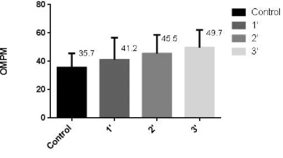
Figure 4.2: Respiration rate: Opercular movements per minute during control vs experiment during the 1st_{, 2}nd_{and 3}rd_minute.

It was observed an upscaling increase in the OMPM, with a 15.4% increase after the first minute compared to the basal control value, a 27.5% increase after the second minute and finally a 39.2% increase after the third minute of the experiment.

During the observations in the Ria Formosa, it was verified for the H. guttulatus an average of 41.2±15.5 OMPM after the first minute of boat transitions, which increased to 45.5±13.3 OMPM after the second minute of transitions and to 49.7±12.5 at the end of the 3rdminute of the observations (persistent sound over the seahorses) (Table 4.1).

Average OMPM ± s.d. Min. OMPM Max. OMPM H. guttulatus

Overall Males Females Overall Males Females Overall Males Females

Control 35.7±10 38.9±9.7 29.8±9.8 13 18 13 62 62 51 1' 41.2±15.5 44.3±15.4 35.5±14.1 20 20 21 71 71 65 2' 45.5±13.3 49.2±13.1 37.8±13.1 21 27 21 76 78 68 3' 49.7±12.5 53.1±14.1 45.3±12.3 31 32 31 82 82 68 H. hippocampus Control 36.6±8.2 34.4±7.3 46.5±2 23 23 43 48 46 48

Table 4.1: Observed average (average±s.d.), minimum and maximum number of OMPM in H. guttulatus and H. hippocampus.

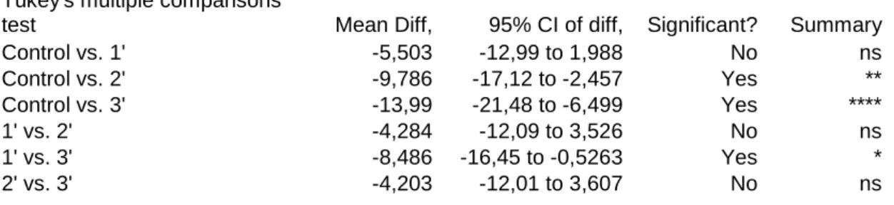
In an overall analysis, H. guttulatus increased their breathing frequency in 8.5 OMPM from the start of the first minute of observations on until the end. This represents almost 4.3 opercular movements’ increase every 20 seconds of respiration in the observed individuals. No matter the slight increase of OMPM, no significant differences (p>0.05) were observed between the number of OMPM of control fish and fish exposed to the transient boat sound during the first minute of observations. However, significant differences were observed from that point on, between the control fish and fish observed during the second (p<0.01) and third minutes of observation (p<0.0001). Concordantly, a significant increase (p<0.05) in OMPM of fish observed in the 1st minute and the 3rd minute was observed (Table 4.2):

Tukey's multiple comparisons

test Mean Diff, 95% CI of diff, Significant? Summary

Control vs. 1' -5,503 -12,99 to 1,988 No ns Control vs. 2' -9,786 -17,12 to -2,457 Yes ** Control vs. 3' -13,99 -21,48 to -6,499 Yes **** 1' vs. 2' -4,284 -12,09 to 3,526 No ns 1' vs. 3' -8,486 -16,45 to -0,5263 Yes * 2' vs. 3' -4,203 -12,01 to 3,607 No ns

Table 4.2: Statistics descriptive of Tukey´s multiple comparisons test between H. guttulatus OMPM control values and data obtained

4.1.2 Observations in the wild (normal boat traffic)

In these observations, just a small number of valid observations were obtained due not only to the random chance of boats passing close to the observed seahorse, but also due to diver’ security issues.

A total of 15 videos were performed between 5.2 and 5.8 meters and 15 animals were observed (11 males and 4 females). Due to technical reasons (identical to the ones mentioned above) within these 15 videos, only 11 animals were able to be used and analyzed for stimuli reaction (site abandon and OMPM measurements). Overall, it was observed an OMPM average of 45.6±10.1, with values ranging between 30 and 70 opercular movements per minute (Table 4.3).

OMPM (average ± s.d.) Min. OMPM Max. OMPM

H. guttulatus

Overall Males Females Overall Males Females Overall Males Females

45.6±10.1 47.4±11.5 42.5±5.8 30 30 36 70 70 53

Table 4.3: Observed average (average±s.d.), maximum and minimum number of OMPM in H. guttulatus.

In a pair-wise comparison with the control data, a significant increase in the OMPM of the wild animals was observed (p<0.05). It was verified a 9.9 OMPM difference (27.7%) between control animals and the ones from the wild (Figure 4.3, Table 4.4).

ANOVA

Variation source SQ Gl MQ F p value Critical F

Between groups 4646.214 4 1161.553 6.82438 4.09882E-05 2.425453 Within a group 28594.68 168 170.2064

Total 33240.9 172 1.974185

Figure 4.3: Opercular movements per minute during control vs observations in the wild

4.2 Hydrophone analysis

In order to perceive the difference between transient sound and constant sound a spectrogram (expressed as frequency per amplitude, thus Hz per dB) was produced using the selected software. Higher sounds perceived as red in the spectrogram corresponded to the boat maximum approximation to the buoy (and therefore to the animals) while blue corresponded to boat moving away from the buoy and fading sound (Figure 4.4).

Figure 4.4: Spectrogram of transient sound of boat passages (top) and constant sound (bottom). 1- Loud sound in red (from boat

approximation); 2- Quiet sound in blue (from boat departure).

During the boat passages a cycle it’s clearly noted: When the trial begins, the boat engage its movement passing near the buoy provoking a loud sound (animals started to increase the OMPM right after the beginning of the trial) represented as red in the spectrogram. As the boat move away from the buoy the sound starts to fade (blue area) and then as the boat returns for the 2ndtransition near the buoy, the sound becomes louder again and so on. (Figure 4.4 – top).

During constant sound observations it was verified that loud sounds prevailed, being red the predominant color throughout all the timeline, fading only when the engine stopped changing to a blue color which corresponded to the end of the observation (Figure 4.4 (bottom).

The frequency analysis allows us to see the differences in the sound produced during the boat transitions and compare it between the moments when the boat was most departed from the buoy (Figure 4.5) to when it was close to it (Figure 4.6). This was achieved through spectrogram analysis, exporting the RMS values (average dBFS) from the red (louder sounds) and blue (lower sounds) zones transforming them into dB and then plot dB per Hz graphs allowing comparisons between each other and also to the one

that corresponded to the red zone (again, the louder sounds’ area) of constant sound’

A distinction is clearly noted between the frequencies analysis of when the boat was far from the buoy to when it was closer. The dB levels were obviously lower when the boat was far from the buoy, varying between 63.4 dB (min.) and 109.4 dB (max.) than when it was the closer (89.8 dB (min.) to 127.6 dB (max.). During constant sound observations, the dB values varied from 82.7 (min.) to 137.1 dB (max.).

Figure 4.5: Example of frequency analysis during boat transitions with the boat departed from the buoy

Figure 4.7: Example of frequency analysis during constant sound with the boat near the buoy

In terms of average sound exposure (RMS) to H. guttulatus, from the first minute to the third, average dB increased from 112.2±2.4 dB to 116.5±3.6 dB with maximum average values ranging from 114.9±2.4 dB to 123.6±3.6 dB (Table 4.5):

Table 4.5: Average (average±s.d.), minimum and maximum sound exposure (in dB) of H. guttulatus observed under natural traffic conditions. × - denote the absence of recorded sound in the control sample. (RMS - root mean signal).

The recorded sound analyzed showed an overall average sound exposure for H.

guttulatus throughout the experience of 112.2±2.4 dB for the 1st minute of boat transitions, 112±3.4 dB for the 2nd _{and 116.5±3.6 dB for the 3}rd _{minute which}

corresponded to constant sound (Table 4.5). Within a RMS average 63.4 dB was the minimum dB value that fish were exposed to (when the boat was at its far off location from the buoy) (Figure 4.5) and 137.1 dB the maximum value (during constant sound observations) (Figure 4.7).

Overall Males Females Overall Males Females Overall Males Females Control

1' 112.2±2.4 111.8±2.3 112.1±1.8 101.8±2 101.8±2.3 106.9±1.8 114.9±2.4 114.2±2.3 114.9±1.8 2' 112±3.4 111.1±4.3 111.7±1.8 94.4±3.7 94.4±4.3 107.8±1.8 115.8±3.4 115.8±3 114.6±1.8 3' 116.5±3.6 116.1±4.4 117.4±3 107.3±3.6 107.3±4.5 112±3 123.6±3.6 123.1±4.5 123.6±3

Average dB of RMS Min. Average dB of RMS Max. Average dB of RMS

4.2.1 Male vs Female respiratory’ rate per dB

It was also verified that when exposed to the same increase in dB’s, males had the tendency to breathe more than females during the entire observation period (Figure 4.8).

Figure 4.8: Comparison between the number of OMPM and respective dB exposure of male and female H. guttulatus during the

observation period.

In fact, it was observed that males have a higher breathing rhythm than females, in all observed situations (Figure 4.9).

Figure 4.9: Comparison of the number of OMPM between male and female H. guttulatus during control, observations in the wild and

On control, where animals are kept in a stressed free environment, males had an average OMPM of 39.9±9.7 and females an average of 29.8±9.8 (Figure 4.10).

Figure 4.10: Comparison of the number of OMPM and standard deviation between male and female H. guttulatus during control

No significant differences (p>0.05) were observed between the number of OMPM between males and females either on control, in the wild or during any point of the observations (Table 4.6):

Tukey's multiple comparisons

test Mean Diff, 95% CI of diff, Significant? Summary Control M vs. Control F 0,2342 -8,061 to 8,529 No Ns

Wild M vs. Wild F 4,929 -19,87 to 29,73 No Ns

1' M vs. 1' F 10,37 -2,936 to 23,67 No Ns

2' M vs. 2' F 11,96 -0,9856 to 24,91 No Ns

3' M vs. 3' F 7,992 -4,784 to 20,77 No Ns

4.2.2 dB per depth

The depths where observations took place were pooled in to depth classes from 4 to 10 meters. Most fish were observed within five meters depth, with a total of 31 from the 60 observations (Table 4.7):

Meters

1 2 3 4 5 6 7 8 9 10

Observed animals

0 0 0 9 31 1 5 8 4 2

Table 4.7: Number of observed animals per depth class

Average OMPM and dB were scored for each depth class (Table 4.8):

Meters OMPM 1' OMPM 2' OMPM 3' dB 1' dB 2' dB 3' H. guttulatus 4 54±12.1 46.8 ±17.1 42.1 ±7.5 128.7 ±4.7 127.3 ±7.8 132±3 5 41.1 ±16.1 47.9 ±14 53±13.1 130.1 ±1.1 129.5 ±3.6 135±3.5 6 21±0 27±0 40±0 130.8 ±0 129.6 ±0 138.1 ±0 7 53±0 46,5±8.5 55.8 ±8.6 131.8 ±0.8 130±2.1 137.7 ±3.4 8 24.8 ±9.9 32.8 ±11.8 30±2 130.2 ±0.9 130.6 ±1.7 132,6±3.5 9 37.3 ±4.5 42±5.4 45.3 ±2.4 128,4±1.1 129.5 ±0.9 135.3 ±3.2 10 23±0 30±0 35±0 128.3 ±3.4 131.4 ±0.9 132.9 ±2.4

Table 4.8: OMPM (opercular movements per minute) and dB per each observation depth class between 4 and 10 meters

Default sound values were also obtained to observe the sound pattern with increasing depths. 30 seconds sound samples per meter were recorded and then analyzed (Table 4.9):

Table 4.9: Default dB per each depth class between 1 to 10 meters.

In the first and second minutes, the OMPM and dBs only get 3 out of 6 and 2 out of 6 transitions (respectively) with a proportional increase or reduction: on the first minute it was only verified a proportional increase from the transition from 6 meters to 7 meters depth, a proportional decrease from 7 meters to 8 meters and a proportional decrease from 9 to 10 meters depth, while on the second minute that is only observed from the 4 to the 5 meters transition and from the 6 to 7 meters transition with proportional increases (Figure 4.11 and 4.12). It was only during the third minute of the experiment, that OMPM and dBs had a proportional increase and reduction in almost every account: 4 out of 6 transitions while increasing depth (Figure 4.13). The sound (in dB) propagated constantly throughout the entire observation periods with one slight residual variations, 2 dB trough the 1st minute, 3 dB from the 2nd minute and 6 dB trough the 3rd (Table 4.8).

It was verified on the default sound measurements (Figure 4.14) that sound increased until 4 meters and then it propagated constantly with just a slight variation of 8 dBs (Table 4.9).

1 2 3 4 5 6 7 8 9 10

140,7±0.4 139,85±4 142,65±0.5 146,7±0.5 147,15±0.7 147,8±3.8 147,55±3.7 146,9±0.7 146,2±0 145,65±0 Meters

Figure 4.11: OMPM and dBs per depth during the first minute of observation under natural conditions.

Figure 4.13: OMPM and dBs per depth during the third minute of observation under natural conditions

5. D

The two European seahorse species, H. guttulatus and H. hippocampus inhabit the Ria Formosa lagoon, where they have been surveyed since the early 2000’s (Curtis & Vincent, 2005; Caldwell & Vincent, 2012; Correia et al., 2014) and where Curtis & Vincent (2005) referenced the bigger seahorse populations irrespectively of the species. However during the last decade (between 2001/2002 and 2008/2009) they suffered a dramatic decrease (Caldwell & Vincent, 2012).

In detail, between 2001 and 2002 Curtis & Vincent (2005) presented estimates of local population abundance, distribution and habitat preference for H. guttulatus and H.

hippocampus. High seahorse densities were found: both species were patchy in

distribution but H. guttulatus mean density (0.073 ind. m–2_{) was one order of magnitude}

greater than that of H. hippocampus (0.007 ind. m–2_{) (Curtis & Vincent, 2005).}

7 years later, Caldwell & Vincent (2012) performed a survey between 2008 and 2009 to identify population changes in H. guttulatus and H. hippocampus in the same locations of the previous study to explore whether there were associated changes in the environment or in habitat use relationships to account for sampling differences between the 2008/2009 surveys and to the 2001/2002 surveys of Curtis & Vincent (2005) where populations in the lagoon were found to be among the densest in the world.

Both seahorse species were absent from 66% of the sites surveyed in the Ria Formosa lagoon in 2008/2009. Between the two species, H. guttulatus was the most common species with an overall density of 0.004 m–2 (± 0.002 S.E.) while H.

hippocampus density was 0.001 m–2 (± 0.0006 S.E.) Both species had declined since 2001/2002, although as mention above the decline was more severe for H. guttulatus. Back in the 2001/2002 survey, H. guttulatus was found in 29 of 32 sites but they had disappeared from 21 sites of those sites by 2008/2009 (Caldwell, 2012).

Figure 5.1: Comparison of densities of H. guttulatus during underwater visual census surveys in 2001/2002 (Curtis and Vincent,

2005) and 2008/2009 (Caldwell, 2012) in the Ria Formosa lagoon (adapted from Caldwell, 2012 PhD thesis).

Overall, the H. guttulatus densities decreased significantly from 0.07 m–2to 0.004 m–2. Population densities of both species had indeed declined significantly between the 2001/2002 and 2008/2009 surveys (94% and 73% for H. guttulatus and H. hippocampus respectively) (Caldwell, 2012) (Figure 5.1).

On a later study by Correia (2014), performed during 2010-2013, 16 of the previously surveyed sites were again surveyed and compared with previous data obtained from those same locations in the two earlier studies (2001/2002 and 2008/2009). Seahorse densities (number of individuals per m2_{), rather than abundances, were compared to}

account for differences in surveyed areas per site in each time period, as it was performed in Caldwell & Vincent (2012). H. guttulatus showed a significant increase in population when compared to the previous 2008-2009 surveys and no significant differences in density where observed when compared to 2001-2002 (Correia, 2014).

Of all the tested variables, (depth, temperature, holdfast coverage) H. guttulatus density only correlated with the percentage of holdfast coverage. The H. guttulatus population seems to be increasing (that may suggest a recovery of this species' population) but still lower than the abundances recorded in 2001-2002 (Correia, 2014).

The short generation time of seahorses, mean that their abundance may fluctuate in response to environmental conditions (Monteiro, 1989; de Silva et al., 2003 in Curtis & Vincent, 2006), making populations vulnerable to declines that could be intensified by high levels of exploitation (King & McFarlane, 2003) in Curtis & Vincent (2006).

Curtis & Vincent (2006) performed a study in the Ria Formosa reporting (among few in situ studies of syngnathid life history) the first mark-recapture estimates of survival

and growth rates for a wild seahorse population. They estimated and cross-validate biological reference points that were indeed important for fisheries management and conservation for H. guttulatus. The results they presented in their study were concordant with inferences based on captive populations and limited field sampling, implying that where field data are lacking, ex-situ studies would be important sources of life-history data for informing conservation policy. They also observed a small fraction (3%) of the population with injuries like punctured brood pouch, clipped tail, missing eye and torn cheek, probably indicating feeding attempts by predators and 7% with small white skin patches accompanied by small black dots, indicating the prevalence of an undetermined disease in this population. On a similar study of Correia et al. (2014) syngnathids were observed in a non-invasive form by means of photo-identification which ultimately led to be a good tool for mark-recapture studies when considering the assessment of seahorses populations and its fluctuations.

They also verified strong site fidelity over space and time for H. guttulatus, coincided with the onset of reproduction and that adult H. guttulatus maintained small home ranges over several years and probably had low emigration rates. The average home range size of adult H. guttulatus on their study was larger than observed in other seahorse species.

Probable causes for this decrease were called into question such as accessory or direct fishing activity (the estimate of the seahorses mortality is possibly derived from exploitation by means of illegal, bottom-dragged fishing gears that are occasionally employed in the Ria Formosa lagoon (Erzini et al., 2002), pollution, environmental degradation and also recreational and human activities that occur in the Ria, generating among other consequences underwater noise pollution.

Due to this issue and to the high vulnerability of the species, CCMAR investigators have been revealing a growing concern regarding the conservations of these species and their habitat, thus developing efforts not only to effectively identify the actual causes for this decrease, but also to test and implement tools to improve and promote the increased complexity of habitats through the creation of artificial structures (Correia et al., 2013; 2014).

There are very few published studies on the effect of sound on seahorses. Although morphologically different from other bony fish, internal organs of seahorses are equal to other bony fish, including the gas bladder so the effect of sound on other fish is likely to be similar in seahorses (Jorge Palma pers. comment).

Captive fish are exposed to ambient noise of water and air pumps, chiller motors of food storage and air bubbles which creates a loud ambient for the animals but literature related to the effects of these noises is poor (Anderson et al., 2011).

Seahorses stress responses to chronic noise exposure have been studied in fish aquariums to score behavioral observations, with tail adjustments and time spent stationary interpreted as irritation behaviors (Anderson et al., 2011).

Noise exposure is also related to hearing, acoustic communication and stress as it may induce hearing loss, affect intraspecific communication (because a loud ambient noise can mask biologically relevant sounds) and trigger stress responses with unfavorable consequences for the animal health, growth and reproduction (Anderson, 2013).

In this study, except for 6 animals, 43 showed visible signs of discomfort throughout the observation period. It was verified that 30.6% of the animals either tried to turn their back or move away from the sound source. Seahorses are cryptic species that always seek to be in contact with holdfasts/shelter only abandoning it in very specific occasions (e.g. feeding in the absence of currents), if they are obliged to do it for other than normal reasons during unsafe situations, for example, during strong current periods, given their poor swimming ability, it can constitute a problem and be a disintegration factor of the population they are included in.

Seahorses are prime examples of sedentary marine fish and being sedentary animals, they can remain within a small area due to easy access of their needed resources: food, shelter/protection, mating opportunities, etc. in that location. Shallow areas of coral reefs or seagrass beds like the Ria Formosa are prone to both natural (e.g. storms, strong currents) and anthropogenic (e.g. fishing, habitat degradation) disturbances. These disturbances may lead to either involuntary displacement of seahorses, or changes in the environment that provokes an immediate response by seahorses to move voluntarily. With dispersal, if fish become displaced far enough from their previous home range they may find themselves unable to return, and thus forced to settle in a new location, which may have a reduced habitat quality and absence of other conspecifics.

A significant increase in the respiration rate of all the 43 observed seahorses was also verified (87.8%). This demonstrates that underwater noise pollution caused by the standard operating boats in the lagoon act as a distress factor to these fish generating an immediate response. It was also verified that animals in the wild tend to breathe significantly more than the ones from control.