Efficient synchronization of one-dimensional chaotic quadratic maps by different couling terms

EFFICIENT SYNCHRONIZATION OF

ONE-DIMENSIONAL CHAOTIC QUADRATIC MAPS BY

DIFFERENT COUPLING TERMS

Dr. Rosário Laureano

, Dr. Diana A. Mendes

, Prof. Dr. Manuel Alberto M. Ferreira

ISCTE -Lisbon University Institute (PORTUGAL)

a,b,c

IBS - ISCTE -IUL Business School, Department of Quantitative Methods

a

[email protected],

[email protected],

[email protected]

The possibility of chaotic systems oscillate in a coherent and synchronized way is not an obvious phenomenon, since it is not possible to reproduce exactly the initial conditions and the sensitive dependence on initial conditions is one of the main characteristics associated with the chaotic behavior. We consider synchronization phenomena of discrete chaotic dynamical systems (identical or non-identical) with nonlinear unidirectional and bidirectional coupling schemes. In order to illustrate the synchronization methods present in this paper, we always use a system of two coupled chaotic quadratic maps. First, we present a systematic way to design unidirectional and bidirectional coupling schemes for synchronizing arbitrary pairs of one-dimensional chaotic maps. In dissipative coupling, we use two methods to study the stability of synchronous state: the linear stability and the Lyapunov functional analysis. Second, we explore other coupling schemes. With the unidirectional coupling based on the singular value decomposition it is possible to suppress the exponential divergence of the dynamics of the synchronization error and to guarantee linear stability of the synchronized state in all points of the state space. The other coupling scheme is asymmetric and appears in natural a family of analytic complex quadratic maps.

Key words: efficient synchronization, one-dimensional chaotic quadratic maps, different coupling terms

INTRODUCTION

Synchronization of dynamical systems is a well-know phenomenon in physics, nature, economics, engine-ering and many other scientific areas. The first observations related to synchronization were reported by Huygens in 1665. In that case, the synchronization was indicated by the equal periods of coupled clocks. Nowadays, syn-chronization is used in a more generalized sense: occurring in periodic and chaotic coupled systems. Coupled dynamical systems are constructed from simple, low-dimensional maps and form new and more complex organizations, with the belief that dominant features of the underlying components will be retained. This building up approach can also be used to create a novel system which behavior is more flexible or richer than that of the components, but which analysis and control remains tractable. One of the main characteristics associated with the chaotic behavior is the sensitive dependence on initial conditions, that is, any infinitesimal perturbations of the initial conditions lead to the divergence of nearby starting orbits. However, when ensembles of chaotic systems are coupled, the attractive effect of a suitable coupling can counterbalance the trend of the trajectories to separate due to chaotic dynamics. As a result, it is possible to reach full or partial synchronization in chaotic systems, depending on the coupling degree. In synchronization we seek subspaces of the coupled system space - the synchronization set - in which a special kind of motion, which relates the coupled system, takes place.

Since the seminal papers of Fujisaka and Yamada (1) and Pecora and Carroll (2), various synchronization methods and several news concepts necessary for analyzing chaos synchronization have been developed. The most well-known regimes of synchronization are the identical (or complete) synchronization, the phase synch-ronization and the generalized synchsynch-ronization. Identical synchsynch-ronization means that the periodic or the chaotic oscillations of the coupled identical systems coincide exactly in time due to the strong interaction between them. Generalized synchronization is a kind of synchronization where exists a one-to-one smooth mapping between oscillations of each subsystem. Hence, knowing the state of one subsystem enables us to know the state of the other subsystem. Phase synchronization is defined as the appearance of a certain relationship between the phases of the coupled systems while the amplitudes can remain uncorrelated.

Coupled dynamical systems in discrete time

Let’s consider the following maps

where and are real dynamical variables, and are chaotic maps and the constants represent the control parameters. Both maps in (1) satisfy a global dissipative condition and hence have a global attractor.

As the dynamics of each map is chaotic, in the case of uncorrelated systems we can observe two independent random-like processes without any mutual correlation. Now let us introduce an interaction between the two systems. Though there are several ways to couple mathematically two maps, we want the coupling to have some relevant properties. The coupling should be dissipative, that is, it tends to make the states and closer to each other, and does not affect the symmetric synchronous state . The proper way to apply a coupling operator to the nonlinear maps (1) is like follows:

where and are the coupling parameters. So, we obtain the coupled system

(2)

as a result of bidirectional coupling. The coupled systems in (2) are synchronized if

as , for a certain range of the control parameters and . The main method of research on this problem is analytical: for given parameter values and , we want to find coupling values of and so that for close initial values and , synchronization must occurs.

The simplest case is the identical synchronized regime, where and . In this case, the system (2) takes the form

. (3)

The coupled system is completely symmetric with respect to changes of the variables , and the coupling parameter is the coupling strength.

This bidirectional coupling scheme can be clearly interpreted in populations light dynamics. One can think of and as simulating the population dynamics of a particular species at two adjacent locations. If the species can migrate in both directions within the time intervals between the stages of their reproduction and death, then represents the fraction of these species, which migrate to the neighboring location, that is, is a measure of the diffusion of individuals between the two locations. For , the phase volume suffers additional contraction in comparison with the magnitude it would have without coupling. This fact gives grounds to call this type of coupling scheme as dissipative coupling.

There are other simple ways to couple two maps. For instance, we could have the linear coupling

, (4) and the bilinear coupling if the linear terms in (4) is replaced by . However, such coupling schemes are not biologically realistic as they involve the mixing of generations: some of the individuals have been allowed to reproduce and die and have also been allowed to move into the other location.

In dissipative coupling, large enough coupling strength should eventually bring about the synchronization of the considered system (3), for any value of . In particular, when , the two variables and are completely independent and uncorrelated, that is, the two systems act independently. For , after few iterations the two variables and become identical and we immediately observe the synchronous state for all . When the synchronous state is reached, the dynamics of both systems corresponds to that of the single map . As the coupling does not affect this state, the dynamics of and are the same as in the uncoupled systems, that is, chaotic. Such a regime, where each of the maps shows chaos and their states are identical at each moment in time, is called full synchronization. So, when the synchronous state is reached, the chaotic dynamics of and are restricted to the one-dimensional invariant attracting subspace , called the synchronization set. Thus, the problem of synchronization can be understood as a problem of stability of a one-dimensional chaotic attractor embedded in the two-dimensional phase space. If we consider the coupling parameter as a bifurcation parameter that increases gradually from , a complex bifurcation structure is generally observed, but one clearly sees a tendency to closer correlation

between the variables and . The goal is to keep the systems as loosely coupled as possible, but still have them synchronize. One can find a critical coupling such that for the synchronous state is established. The synchronization near this the coupling threshold appears to be highly sensitive. The points outside the diagonal represent the non-synchronous state. With the increasing of , the distribution of the points tends towards the diagonal, and beyond the critical coupling all points satisfy . The critical coupling value is obtained from the Lyapunov exponent of the uncoupled chaotic system.

Stability analysis of the synchronous state in dissipative coupling Linear stability analysis

The coupling threshold in which we obtain stable synchronous state in (3) can be computed by the linearization around the synchronous state, where . To characterize the synchronization transition at

, it is convenient to define two new variables

and Geometrically, the variable is directed along the diagonal , while the variable corresponds to the direction transverse to this diagonal. In the synchronous state, and

. Close to the synchronous state, the variable is small and its evolution will determine the stability of the synchronous state. Note that, since system (3) remains invariant under the transformation , the synchronous state is a solution of (3) for all values of . So , if the initial conditions are symmetric, , the symmetry is preserved in time. If we want the synchronous state to be observed not only for specific, but also for general initial states, we must impose the stability condition: the full synchronous state should be an attractor, that is, synchronization should establish even from non-symmetric initial states. This stability condition will give us the critical coupling for the onset of synchronization. The rate of growth of a small difference along two trajectories on the chaotic attractor is measured through the Lyapunov exponent and the evolution of perturbations in the perpendicular direction, which determines the stability of the synchronous attractor, is characterized by the transversal Lyapunov exponent .

The system (3) can be written in the form

.

We make this system linear near the synchronous state , where the variable is small, and obtain a couple of linear maps for small perturbations of and given by

and (5)

where the derivative is evaluated along the synchronous state. Since in the linear approximation the perturbations of and do not interact, the perturbations can be treated separately. For

, the Lyapunov exponent is nothing else than the Lyapunov exponent for the uncoupled map

and the transversal Lyapunov exponent can be written in terms of in the following simple way: . Because of this simple dependence on , the boundary of stability of the synchronous state can be immediately deduced: the synchronous state is stable if the Lyapunov exponent corresponding to the difference variable is negative, that is (and unstable if ), and the range of stability is given by

. The coupling threshold is then defined from the condition , that is

.

Global stability analysis

Global stability in a neighborhood of an equilibrium point is confirmed if there exist a positive definite function defined in that neighborhood, whose derivative is negative semi-definite (3). To get conditions for the

global stability of synchronization of two systems in variables x and y, we define the associated Lyapunov function by

.

Since , the equality holds only when the systems are exactly synchronized. For the asymptotic global stability of the synchronous state, the Lyapunov function should satisfy the following condition in the region of stability,

. (6) If we consider the coupling scheme (3), the Lyapunov function is written as

and, using the Taylor expansion of about , we obtain

(7)

If the expression in the square bracket on the right hand-side is bounded then always exist some values of around for which the synchronous state will be stable.

As an example, consider now the bidirectional coupling scheme (3) with the one-dimensional quadratic

map ,

where is the control parameter. The map defines a discrete dynamical system

whose behavior has been intensively studied. The system obtained by coupling exhibits a much richer dynamics that the single quadratic map, but is still simple enough to allow the study of its behavior. In what follows we will always consider higher than the Misiurewicz point (Figure 1), where the quadratic maps are chaotic. 0 1 2 0 0.5 2 X: 1.565 Y: 0.8111 a x

Figure 1. Bifurcation diagram of the one-dimensional quadratic map .

By (7) the corresponding Lyapunov function leads to

, that is,

. Hence, it follows that we have the approximation

,

and onsidering , we obtain

and finally, by the synchronization condition (6) we have that is, . Moreover, if we consider a more realistic bound for as , a better range for can be obtained

In order to illustrate the efficiency of this synchronization method we consider some numerical simulations with chaotic maps.

-1 -0.5 0 0.5 1 1.5 2 -2 -1 0 1 2 50 100 150 200 250 300 350 -1 0 1 2

Figure 2. Dissipative coupling (3) with , , and : (a) hyperplane

of synchronization, (b) time series

For example, if , and different initial conditions ,

, the synchronization takes place after few steps ( iterations). Figure 2 illustrates the stabilization of the dynamics of the coupled system on the synchronization set . The transition points ( iterations) are the points outside the attractor. We also represent the time series of the and variables and the error . For any value of closer to the critical threshold the synchronization is attained in the shorter time interval.

Unidirectional coupling based on singular value decomposition

Consider two identical chaotic dynamical systems and , where

is the control parameter. We want to synchronize these systems by using a unidirectional dissipative coupling, that is

, (8) where , depending on , is the coupling matrix that suppresses the local expansion of the flow along the non-contracting directions. In this unidirectional coupling, and are the real dynamical variables of the drive (or master) and the response (or slave) systems, respectively. The expression is called the coupling term. As we see, in unidirectional coupling only the dynamics of the response system is affected by the drive system through the coupling; the reverse does not hold.

Junge and Parlitz (3) show that the synchronization of chaotic systems can be explained by the suppression of expanding dynamics in the state space transversal to the synchronization manifold . For that, it was considered the singular value decomposition (SVD) of the Jacobian matrix,

,

where and are orthogonal matrices and is a diagonal matrix with positive elements , represented by the singular values of . Thus, we can use one of the most powerful coupling schemes defined by

where we assume that exist local non-contracting directions at and are the column

vectors of with corresponding singular values . Note that, choosing

,

the matrix governing the synchronization error dynamics , yielding by (8) as

, is given by the singular value decomposition

,

where appear only singular values that are smaller than . So that, the choice of this matrix guarantees the linear stability of the synchronous state. With this method, systems can be synchronized using a minimum of transmitted information. In fact, Junge and Parlitz (3) have showed that this scheme coupling allows for breaking the coupling from time to time in order to reduce the information flow from the drive to the response system. They discuss two ways to exploit this feature: by sporadic coupling (where iterations are performed before the next coupling signal is computed from the current state and transmitted to the response system where it is applied in the coupling) and in partitioned state space (the singular values de depend, in general, on the state , so one may restrict the coupling to the regions in the state space where strong expansion has to be suppressed).

To show the efficiency of the proposed coupling, in deficit to linear coupling, we consider again the one-dimensional quadratic map . The singular value of the Jacobian matrix of is given by the square root of the eigenvalue of the matrix . Thus, we have the characteristic equation

and the singular value is . For we observe chaotic

motion for the quadratic map. Then we find a positive Lyapunov exponent and the singular value satisfy

, when , indicating expansion. Choosing the coupling constant

, the coupling term can be written as

, and the coupling scheme is given by

In practical simulation the synchronization is achieved in a very short time. With and the

initial conditions , we obtain the Figure 3.

The first question we want to address with this example is how much the approximation of the local singular values and vectors at the response system degrades the performance of this coupling. For this purpose we have compared the coupling given below with a corresponding coupling given by linear and quadratic coupling. We can observe that for the similar initial conditions and parameter settings, the synchronization is achieved after more than iterations. This is very important since in economical or biological systems the expenses to apply these synchronization techniques are very elevated and not practical if the time to achieve synchronization is very large.

Bidirectional coupling based on complex quadratic maps

Consider the family of analytic complex quadratic maps defined by

, where we proceed to the decomposition into real and imaginary parts. Further

considering and , we obtain

According to Isaeva et al. (4), the variable and parameter changes , ,

this is equivalent to the simplified form

(9)

where . In (9) we have an asymmetric coupling between two one-dimensional

quadratic maps, where is the coupling strength and is the nonlinear coupling term. The constants and are the control parameters of the subsystems in coupling.

-1 -0.5 0 0.5 1 1.5 -1 -0.5 0 0.5 1 1.5 0 10 20 30 40 50 60 70 80 90 100 -1 0 1 2

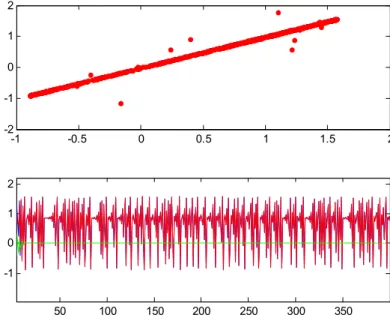
Figure 3. Unidirectional coupling given by SVD with , and : (a)

hyperplane of synchronization, (b) time series.

Consider the coupled system (9) with ,

(10) In this case, the difference evolves with respect to the difference equation defined by

The equation is equivalent to

.

Proposition: For each fixed value of and initial conditions and such that , there is an

interval of values of for which stable asymptotic synchronization in the coupled system (10) is achieved.

For any the difference explodes to infinity. Let the control

parameter in the coupled system (10). In the next table the interval for some values of is presented:

The amplitude of the intervals decreases when the difference between the initial

conditions and increases. If , in decimal step, all the intervals have

as superior extreme. If , in decimal step, the stable asymptotic synchronization is achieved only for . So, it was guaranteed the stable synchronization in the coupled system (10) for

for all the symmetric initial conditions, even if the distance between them is a high value (Figure 4). A small deviation on the value of a leads to a change in the interval .

0 1 2 3 4 5 6 7 8 9 10 -1000 -500 0 500 N x , y , y -x

a=1.97, parâmetro de ligação 0.25

X: 2 Y: 0 -100 0 100 200 300 400 500 -600 -400 -200 0 200 x y

Figure 4. Bidirectional coupling in (10) taking : (a) time series, (b) hyperplane of

synchronization

Now consider initial conditions and such that . For example and .

If the difference is bounded to an interval . The amplitude of the interval

increases with . If the amplitude of is smaller than , so it is

achieved practical synchronization in the Kapitaniak sense for these values of . At the

synchronization error varies in the interval of minimal amplitude.

REFERENCES

1. H. Fujisaka and T. Yamada, Stability theory of synchronized motion in coupled oscillator systems, Prog. Theor. Phys. 69 (32), 32, (1983)

2. L. M. Pecora and T. L. Carrol, Synchronization in chaotic systems, Phys. Rev. Lett. 64 (8), 821, (1990) 3. L. Junge and U. Parlitz, Synchronization using dynamic coupling, Phys. Rev. E 64, 1, (2001)

4. O.B. Isaeva, S.P. Kuznetsov and V.I. Ponomarenko, Mandelbrot set in coupled logistic maps and in an electronic experiment, Phys. Rev. E 64, R055201-4, (2001)