Acta Scientiarum
http://www.uem.br/acta ISSN printed: 1679-9275 ISSN on-line: 1807-8621
Doi: 10.4025/actasciagron.v39i1.28535
Modeling the incidence of citrus canker in leaves of the sweet
orange variety ‘Pera’
Danielle da Silva Pompeu1*, Terezinha Aparecida Guedes1*, Vanderly Janeiro1, Aline Maria
Orbolato Gonçalves-Zuliane2, William Mario de Carvalho Nunes2 and José Walter Pedroza
Carneiro2
1
Departamento de Estatística, Universidade Estadual de Maringá, Av. Colombo, 5790, 87020-900, Maringá, Paraná, Brazil. 2Departamento de Agronomia, Universidade Estadual de Maringá, Maringá, Paraná, Brazil. *Authors for correspondence.
E-mail: danielle11silva@gmail.com; taguedes@uem.br
ABSTRACT. Citrus canker, caused by the bacterium Xanthomonas citri subsp. citri, is one of the most important diseases of citrus. The use of resistant genotypes plays an important role in the management and control of the disease and is the most environmentally sustainable approach to disease control. Citrus canker incidence was recorded in an experiment on nine genotypes of the sweet orange variety ‘Pera’ grafted on four rootstocks. The experiment was started in 2010 and the incidence of citrus canker on the leaves was recorded on a quarterly basis. The incidence data from the experiment were analyzed using a zero-inflated Beta regression model (RBIZ), which is the appropriate method to describe data with large numbers of zeros. Based on the residual analysis, the data fit the model well. The discrete component of the explanatory variable, rootstock, was not significant as a factor affecting the onset of disease, in contrast with the continuous component, genotype, which was significant in explaining the incidence of citrus canker.
Keywords: zero-inflated Beta distribution, mixture models, inflated Beta regression model, modeling proportions.
Modelagem da incidência de cancro cítrico em folhas de laranja doce variedade Pera
RESUMO. O cancro cítrico, causado pela bactéria Xanthomonas citri subsp. citri é uma das doenças mais importantes da citricultura. A utilização de genótipos resistentes à doença assume um papel importante no manejo e controle do patógeno, sendo essa uma medida viável ao produtor e sustentável ao ambiente. O conjunto de dados utilizado neste trabalho consistiu das observações obtidas de um experimento em que foram empregados como material vegetal, nove genótipos de Laranja doce, variedade Pera enxertado em quatro diferentes porta-enxertos. Este experimento teve inicio em 2010 e foram realizadas avaliações trimestrais para determinar a incidência de cancro nas folhas das plantas. Para a análise dos observações resultantes desse experimento foi utilizado a regressão Beta inflacionada de zero (RBIZ), que é a metodologia adequada para descrever proporções com grandes quantidades de zeros. A partir da análise residual, pode-se perceber que os dados se apresentaram de maneira homogênea indicando um bom ajuste do modelo. Para o componente discreto a variável explicativa, porta enxerto, foi significativa para o não aparecimento da doença, em contraste com o componente contínuo, em que a variável genótipo mostrou-se significativa para explicar a incidência de cancro cítrico.
Palavras-chave: distribuição Beta inflacionada no ponto zero, modelo de mistura, modelo de regressão Beta inflacionado, modelagem de proporções.
Introduction
According to Gonçalves-Zuliani, Nunes, Zanutto, Filho, and Nocchi (2015), citrus canker caused by Xanthomonas citri subsp. citri (Xcc, Schaad et al., 2006) is an important disease in many citrus-producing regions of the world (Gottwald et al., 2002). Xcc can cause disease in many commercial varieties of citrus, specifically sweet orange (Citrus sinensis L. Osbeck), resulting in significant economic losses to the producer. In addition to direct yield loss, the lesions caused by citrus canker can preclude
the marketing of fresh fruit. In Brazil, citrus canker has been studied by several authors including Carvalho et al. (2015); Gonçalves-Zuliani et al. (2015) and Braido et al. (2015). The search for genotypes resistant to citrus canker is the most attractive way to control this disease as it has least environmental impact (Gonçalves-Zuliani et al., 2015).
orange. According to these authors, rootstock influenced the tolerance of the canopy to plant disease; in general, the rootstocks that induced less prolific growth in the scion showed a lower incidence of disease compared with the rootstocks that induced more vigorous growth. In this case, the effect was estimated from the total count of leaves and diseased leaves; thus, the resulting data set had a high proportion of zeros, that is, the data were zero-inflated. For analysis, Gonçalves-Zuliani et al. (2015) used a non-parametric statistic and later applied Tukey’s HSD test, without taking into account the large proportion of zeros in the data or the correlation due to repeated measures. The conclusion was that grafted genotypes of sweet orange showed a range in the incidence of diseased leaves, with those scions on Rangpur lime rootstock being the most susceptible to the pathogen, possibly due to increased canopy vigor due to this rootstock.
In the current experiment, the objective was to evaluate the functional relationship of dependent variables to one or more predictor variables (Neter, Kutner, Nachtsheim, & Wasserman, 1996). Many regression models have been proposed in statistical modeling, but the most common is the classic regression model or the linear model. In this case, the relationship between variables is described by a linear function assuming independence and normality of errors. These models, however, are inappropriate when the dependent variable is a rate, ratio, or fraction with the records contained in one of these limited ranges: ([0, 1), (0, 1] and [0, 1]). In these cases, the estimates obtained by using the classical regression model may exceed these limits. Thus, it is recommended that the response variables be transformed to avoid this discrepancy to allow the estimates to conform to the linear model. However, data transformation can make the interpretation of the model parameters difficult in relation to the original response.
An alternative method to fit a regression model for continuous variables is to assume a probability distribution to describe the data. The Beta distribution is appropriate for modeling binary, zero-inflated data (0, 1). Several reports describe the fitting of regression models for response variables using the Beta distribution. For example, Ferrari and Cribari-Neto (2004) developed a regression model where the response variable was described by the Beta distribution and the average response was described by a linear predictor using a linking function. The authors reparameterized the Beta distribution to facilitate their interpretation by
indexing using mean and dispersion parameters. Consequently, the model is useful when the dependent variable has its values in the interval (0, 1) and they are related to other predictor variables. Furthermore, other researchers such as Paolino (2001) have used the Beta regression to compare the estimates obtained using Beta regression models and linear regression with and without transformation of the dependent variable. The estimates of the Beta distribution have significant advantages over the linear model in those cases where the response variable assumes values in the interval (0, 1). Pereira, Souza, and Cribari-Neto (2014) have effectively used the inflated Beta regression model to assess the administrative efficiency of Brazilian municipalities to compare the performance of each region with respect to the management of public resources.
However, there are situations in which the variable of interest assumes values at one or both ends of the range, i.e., [0, 1), (0, 1] and [0, 1]. In these cases, the use of the Beta distribution is not feasible and a mixture model using discrete and continuous distributions has been recommended. The discrete distribution estimates the probability mass at zero, one, or both, and the continuous distribution describes the continuous component of the data. This type of model is known as an inflated model. Ospina and Ferrari (2010) introduced the Beta distribution inflated distributions that mix the Beta distribution with the Bernoulli distribution to estimate the mass of probability of zero, one, or both. This family of distributions is formed by the parameterization of the Beta distribution and by the distribution that will describe the discrete component.
We propose an alternative analysis to the report by Gonçalves-Zuliani et al. (2015), considering an evaluation of genotype response due to the presence of correlations between the repeated observations and the large proportion of zeros in these data. The objective of this study was to apply an inflated regression model to describe the incidence of citrus canker on leaves of different genotypes of sweet orange, variety Pera, taking into account the different rootstocks and their effects on the susceptibility of the sweet orange genotypes to citrus canker. Thus, the same data set as that described by Gonçalves-Zuliani et al. (2015) was used here.
Material and methods
Experimental data
Modeling the incidence of citrus canker 3
the variety Pera were grafted onto four rootstock genotypes (Table 1) and planted (2.5 × 6.0 meters). The trees received fertilizer containing N, P, K and foliar Zn and Cu following standard recommendation. Insecticide sprays were applied to control false spider mites (Brevipalpus phoencis), citrus rust mite (Plyllocoptruta oleivora), citrus red mite (Panonychus citri), psyllids (Diaphorina citri), scale insects (Selenaspidus articulates, Parlatoria sp., Unapis citri, Orthezia praelonga, Coccus sp.), fruit-fly (Ceratitis capitata) and orange fruit borer (Ecdytolopha aurantiana). Additionally, fungicide sprays were applied to prevent anthracnose (Colletotrichum acutatum) and scab (Sphaceloma fawceti), and copper bactericidal sprays were applied for the management of citrus canker (Gonçalves-Zuliani et al., 2015).
Approximately two-year-old plants were assessed quarterly to determine the incidence of citrus canker on the leaves. Gonçalves-Zuliane et al. (2015) selected 10 plants per genotype and four branches from each plant. We only used one of the evaluations to perform the analyses proposed. The total leaf number and the number of diseased leaves were counted on each branch such that the total sample size was n = 360.
Statistical analysis
The percentage incidence of canker-infected leaves on the different genotypes of Pera sweet orange was analyzed using the Beta distribution, which has been widely used for modeling when data are in the range (0, 1). However, because the incidence of citrus canker can take values in the interval [0, 1), it was necessary to make some changes in the analysis. Thus, the distribution that was used was the inflated Beta distribution following the modification suggested by Ferrari and Cribari-Neto (2004).
The parameterization of the Beta distribution suggested by Ferrari and Cribari-Neto (2004) to describe a random variable Y restricted in range (0, 1) has a density function given by:
1 (1 ) 1
y
( )
f (y; , ) y (1 y)
( ) ((1 ) )
µφ− −µ φ− Γ φ
µ φ = −
Γ µφ Γ − µ φ (1)
Thus, Y follows a Beta distribution function with the average parameter μ, precision φ and is denoted by Y B(μ, φ). The respective mean and variance of Y in this parameterization are E[Y]=μ and
Var( ) Var[Y]
1 µ =
+ φ , where Var(μ)= μ(1-μ) is the variance function.
The cumulative distribution function using the mixture model of the Beta distribution with degeneration at zero, one or both is given by:
{c} {c}
BI (y; , , )α µ φ = αI (y) (1+ − α)F(y; , )µ φ (2)
in which IA(y) is an indicator function that assumes the value 1 if y ∈A, or 0 otherwise, and A is the set of elements for the value y = c; F(.; μ, φ) is the cumulative function of the Beta distribution; α=P(y=c) is the parameter of the mixture distribution 0<α<1. As BI{c} has a mass point at y = c, it cannot be considered completely continuous. Note that with a probability α, the variable Y is selected from a degenerate distribution at c, and when the probability is (1-α), the variable is selected from a Beta distribution. The probability density function of the variable Y is given by the value generated by the mixture model and is written in the following form:
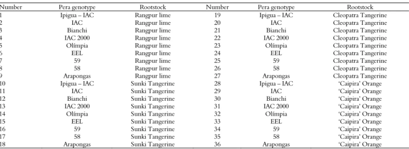
Table 1. Pera sweet orange genotypes grafted on rootstocks of Rangpur Lime, Sunki Tangerine, Cleopatra Tangerine and ‘Caipira’ Orange.
Number Pera genotype Rootstock Number Pera genotype Rootstock
1 Ipigua – IAC Rangpur lime 19 Ipigua – IAC Cleopatra Tangerine
2 IAC Rangpur lime 20 IAC Cleopatra Tangerine
3 Bianchi Rangpur lime 21 Bianchi Cleopatra Tangerine
4 IAC 2000 Rangpur lime 22 IAC 2000 Cleopatra Tangerine
5 Olímpia Rangpur lime 23 Olímpia Cleopatra Tangerine
6 EEL Rangpur lime 24 EEL Cleopatra Tangerine
7 59 Rangpur lime 25 59 Cleopatra Tangerine
8 58 Rangpur lime 26 58 Cleopatra Tangerine
9 Arapongas Rangpur lime 27 Arapongas Cleopatra Tangerine
10 Ipigua – IAC Sunki Tangerine 28 Ipigua – IAC ‘Caipira’ Orange
11 IAC Sunki Tangerine 29 IAC ‘Caipira’ Orange
12 Bianchi Sunki Tangerine 30 Bianchi ‘Caipira’ Orange
13 IAC 2000 Sunki Tangerine 31 IAC 2000 ‘Caipira’ Orange
14 Olímpia Sunki Tangerine 32 Olímpia ‘Caipira’ Orange
15 EEL Sunki Tangerine 33 EEL ‘Caipira’ Orange
16 59 Sunki Tangerine 34 59 ‘Caipira’ Orange
17 58 Sunki Tangerine 35 58 ‘Caipira’ Orange
{
I{c}(y) 1 I{c}(y)}{
1 I{c}(y{c}
bi (y; , , )α µ φ = α (1− α)− f(y; , )µ φ − (3)
where 0<α<1, , φ>0, and f(.; μ, φ) is the density function in Equation (1) (Ferrari and Cribari-Neto, 2004). If α>0, the probability mass distribution at Beta point y = c is exceeded, i.e., the probability of observing y = 0 or y = 1 is α=P(y=c). Note that the first term of the distribution shown in Equation (3) depends on (α), and the second term depends on (μ, φ) because it involves the continuous part of the response variable (Ospina & Ferrari, 2010).
The expected mean and the variance of Y following the inflated Beta distribution are given
by: E[Y]=αc+(1-α)μ and (1 )
Var[Y] (1 ) 1 µ − µ = − α
+ φ ,
respectively. Thus, E[Y]ˆ = α +ˆc (1− α µˆ ˆ) estimates the response of the inflated Beta model. The distribution shown in Equation (3) for Y in the interval [0, 1) is nominated an inflated Beta distribution at point zero (BIZ), and denoted by =Y BIZ(α, μ, φ). In this analysis, the case will be discussed based on the observed values in the range [0, 1) (0 ≤ y < 1).
On account that Y1, ..., Yn are independent random variables, in which Y1, i=1, ..., n, follows the distribution at the inflated Beta c point (c = 0 or c = 1) as in Equation (2), i.e., Yt BI{c}(αt, μt, φ), the inflated Beta regression model (RBIc) is defined by the systematic components:
M
t ti i t
i 1
h(
)
Z
=
α =
γ = ζ
m
t ti i t
i 1
g(
)
X
=
µ =
β = η
in which Zt1, ..., ZtM and Xt1, ..., Xtm are observations from known regression variables with M+m<n. For discrete components of the inverse probit link function αt=Φ{ζt}, and for the continuous model, the inverse of the log link function is μt=exp{ηt}. We note that μt is the conditional average of yt to y∈(0, 1) and φ is the dispersion parameter that can be variable or constant for all of the observations.
In the model RBIc, the estimate of the parameters vector θ=(γT, βT, φ)T can be calculated using the maximum likelihood method whose function is given by:
( ) { }( ) 1( ) (2 )
1
L θ bi y ; α, μ, L γ L β, ,
n
c t t t
t
φ φ
=
=
∏
=wherein,
( )
{ }( )(
)
1 { }( )1
1
L γ α c t 1 α c t , n
I y I y
t t t − = =
∏
− ( ) ( ) ( ) 2t:y 0,1
L β, f y ; μ, .
t
t t
φ φ
∈
=
∏
However, as these estimators do not have a closed form, they may be obtained by maximizing the log-likelihood function using a nonlinear optimization algorithm, such as a Newton algorithm or a quasi-Newton algorithm (Ferrari & Cribari-Neto, 2004). We used the package gamlss
(Generalized Additive Models for Location, Scale and Shape) from the statistical program R to obtain point estimates for the parameters of the RBIZ model.
Various measures of “goodness of fit” can be evaluated, and the model of fit assessment can be based on the estimated values for the maximum likelihood from the sample. One of these goodness of fit values is the pseudo R2 of McFadden (1973),
given by: 2 θ 0
l
ρ
=1-l
,
where lθ is the log-likelihood function of the fitted model and l0 is a function of the log-likelihood of the null model, or the model without the regression structure. Based on Louviere, Hensher, and Swait (2000), the model has the best goodness of fit when the value of ρ2 ranges from 0.2 to 0.4. Domencich and McFadden (1975) ran simulations to compare the range of ρ2 with multiple correlation coefficients of the range (R) and found that the range of ρ2 (0.2 to 0.4) is equivalent to an R range of 0.7 to 0.9.
Based on Ospina and Ferrari (2012), the residual analysis of a regression model inflated with zeros should be divided into two parts: the first evaluates residuals of discrete components (rD
pt) and the
continuous (rC
pt) model. These authors propose that
Modeling the incidence of citrus canker 5
(2012) suggested a standardized version of the Pearson residual. For the continuous component, they followed Espinheira, Ferrari, and Cribari-Neto (2008) to set a weighted version of the common residual of Fisher's iterative algorithm score used to estimate the parameter β when φ is fixed. A more detailed discussion can be found in Ospina and Ferrari (2012).
Results and discussion
Initially, an exploratory analysis of canker incidence was performed for each genotype and rootstock. All zeros were removed from the data set. Based on these data, the genotype Arapongas developed the highest incidence of citrus canker (Figure 1). Considering rootstock effects, the ‘Caipira’ orange (Figure 2) rootstock appeared to support the lowest incidence of citrus canker in the scion (regardless of scion genotype).
Figure 1. Box-plot of the incidence of citrus canker on leaves of different genotypes of sweet orange Pera (Citrus sinensis).
Figure 2. Box-plot of the incidence of citrus canker on leaves of scions of sweet orange Pera (Citrus sinensis) on four different rootstocks.
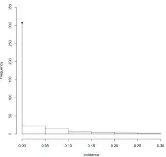
However, the distribution of the variable incidence is asymmetric – there is a high proportion of zeros in these data, Figure 3. Approximately 85.28% of these data are zeros, which justifies the use of the zero-inflated model.
In Figure 3, the incidence of citrus canker can be described by an inflated Beta distribution. Therefore, an RBIZ model was used and adjusted with Yi BIZ(α, μ, φ) as Equation (2), including the covariates rootstock and genotype in the model as follows:
Figure 3. Frequency of incidence of citrus canker on leaves of the sweet orange variety Pera (Citrus sinensis).
( ) 0 1 2 3 4
5 6 7 8
9 10
11
2000 58 59
Probit α γ γ Bianchi γ EEL γ IAC γ IAC
γ Ipigua IAC γ G γ G γ Olímpia
γ Limão Cravo γ Tangerina Cleópatra
γ Tangerina
= + × + × + × + ×
+ × − + × + × + ×
+ × + ×
+ × Sunki
(4)
and
( ) 0 1 2 3 4
5 6 7 8
9 10
11
2000
58 59
Log Bianchi EEL IAC IAC
Ipigua IAC G G Olímpia Limão Cravo Tangerina Cleópatra
Tangerina Sun
= + × + × + × + ×
+ × − + × + × + ×
+ × + ×
+ ×
µ β β β β β
β β β β
β β
β ki.
(5)
These equations represent sub-models and are the discrete and continuous components, respectively, in the model described by Equation (2). To fit these models, we used the gamlss
However, some parameters in the two sub-models were not significant, (Table 2). Therefore, we used the Akaike information criterion (AIC) to select the most appropriate reduced model (using
stepGAIC in module gamlss in R).
The AIC value for the reduced model was 124.7. The McFadden pseudo R2 for this model was estimated at ρ =ˆ2 0.271, indicating a good fit. The test of the likelihood ratios (LR) indicated that there was no evidence to reject the null hypothesis (H0:(γ1=...=γ8=0); (β9=β10=β11=0)), i.e., these parameters were not significant in the model (at the 5% level), with the statistical test LR = 15.1 and p -value = 0.3.
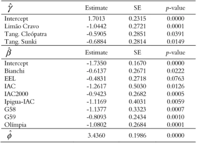
The observed estimates and their standard errors for the reduced model are presented in Table 3. For the sub-model Probit(α) (4), the estimates of the discrete component regression parameters were significant for the variable rootstock. The estimates for the sub-model Log(μ) (5), the continuous component of the model, and the parameters were significant for all genotypes of the sweet orange variety Pera.
Based on the Probit(α), sub-model (6), the rootstock ‘Caipira’ orange induced the most resistance in the scion to citrus canker. ‘Caipira’ orange was followed by Cleopatra tangerine, Sunki tangerine and rangpur lime in increasing incidence of canker on the scion.
The Log(
µ
), sub-model (7), indicated that the genotype Arapongas had the lowest incidence of citrus canker, followed by genotypes IAC and G58.The genotypes EEL and Bianchi were more susceptible to citrus canker.
Table 3. Estimates and standard errors of the regression using the zero-inflated Beta model.
ˆ
γ Estimate SE p-value
Intercept 1.7013 0.2315 0.0000
Limão Cravo -1.0442 0.2721 0.0001
Tang. Cleópatra -0.5905 0.2851 0.0391
Tang. Sunki -0.6884 0.2814 0.0149
ˆ
β Estimate SE p-value
Intercept -1.7350 0.1670 0.0000
Bianchi -0.6137 0.2671 0.0222
EEL -0.4831 0.2718 0.0763
IAC -1.2617 0.5030 0.0126
IAC2000 -0.9423 0.2682 0.0005
Ipigua-IAC -1.1169 0.4031 0.0059
G58 -1.1377 0.3323 0.0007
G59 -0.8093 0.2434 0.0010
Olímpia -1.0802 0.2684 0.0001
ˆ
φ 3.4360 0.1986 0.0000
Note: SE - Standard Error.
The reduced model has the following sub-models:
1.7013 1.0442 0.590
0.68 (
8 )
4
- Limão Cravo - 5Tangerina Cleópatra Tangerina
Probit
Sunki,
= α
(6)
and
1.7350 0.6137 0.4831 1.2617 0.9423 1.1169 1.1377 0.8093 1.08 2 . )
0 ( - - - EEL - -
Log Bianchi IAC IAC2
- - -
000 Ipigua-IAC G58 G59 Olímpia
= µ
(7)
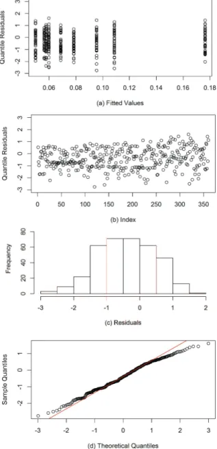
Measures of model fit, Figure 4, show that (a) the residuals were randomly scattered around zero, (b) the points were in the range from -3 to 3, and (c) and (d) the residual distribution function approximated the normal.
Table 2. Estimates and standard errors of the zero-inflated Beta regression model to predict the incidence of citrus canker on sweet orange leaves.
ˆ
γ Estimate SE p-value βˆ Estimate SE p-value
Intercept 1.8974 0.3583 0.0000 Intercept -1.8892 0.3518 0.0000
Bianchi -0.1841 0.3653 0.6146 Bianchi -0.5312 0.2781 0.0570
EEL -0.0147 0.3794 0.9692 EEL -0.4288 0.2728 0.1170
IAC 0.4663 0.4350 0.2845 IAC -1.1147 0.5225 0.0336
IAC2000 -0.3787 0.3555 0.2875 IAC2000 -0.8456 0.2741 0.0022
Ipigua-IAC 0.2716 0.4072 0.5053 Ipigua-IAC -0.9805 0.4024 0.0153
G58 -0.0107 0.3799 0.9775 G58 -1.0994 0.3272 0.0009
G59 -0.5576 0.3491 0.1112 G59 -0.7041 0.2511 0.0053
Olímpia -0.4349 0.3553 0.2219 Olímpia -1.0704 0.2691 0.0001
Limão Cravo -1.1102 0.2852 0.0001 Limão Cravo 0.2123 0.3181 0.5050
Tang. Cleópatra -0.6418 0.2974 0.0316 Tang. Cleóp 0.0313 0.3405 0.9268
Tang. Sunki -0.7515 0.2934 0.0109 Tang. Sunki -0.0818 0.3304 0.8046
ˆ
φ 3.4870 0.1985 0.0000
Note: SE - Standard Error.
Modeling the incidence of citrus canker 7
Figure 4. Measures of model fit. (a) fitted values versus quantile residuals; (b) index versus quantile residuals; (c) histogram of residual frequency; (d) quantile-plot.
To check the outliers of the RBIZ model, we reviewed the residuals (rD
pt) and (rCpt). For the
discrete component (Probit(α)), observations 291, 305, 332 and 340 exceeded the range of -3 to 3 and are outliers (Figure 5 (a) and (b)); (Figure 5 (c) and (d)) represent the continuous component. These observations are the same as the outliers in the box-plot, Figures 1 and 2. In Figure 5 (c) and (d), the points are in the range from -3 to 3.
With the exclusion of observations 291, 305, 332, and 340, the estimates do not differ from those that include all of the observations. Therefore, they should not be excluded from the analysis.
Figure 5. Model fit in relation to outliers. (a) and (b) represent the discrete component; (c) and (d) represent the continuous component.
Conclusion
Acknowledgements
The authors thank the referees for their valuable comments and suggestions on this article and the National Council for Scientific and Technological Development (CNPq).
References
Braido, R., Gonçalves-Zuliani, A. M., Nocchi, P. T., Junior, J. B., Janeiro, V., Bock, C. H., & Nunes, W. M. (2015). A standard area diagram set to aid estimation of the severity of Asiatic citrus canker on ripe sweet orange fruit. European Journal of Plant Pathology, 141(2), 327-337.
Carvalho, S. A., Nunes, W. M. de C., Belasque JR, J., Machado, M. A., Croce-Filho, J., Bock, C. H., & Abdo, Z. (2015). Comparison of Resistance to Asiatic Citrus Canker Among Different Genotypes of Citrus in a Long-Term Canker-Resistance Field Screening Experiment in Brazil. Plant Disease, 99(2), 207-218. Domencich, T., & Mcfadden, D. (1975). Urban travel
demand: a behavioural approach. Amsterdam, NL:
North-Hollan Publishing Co.
Espinheira, P. L., Ferrari, S. L. P., & Cribari-Neto, F. (2008).
Influence diagnostics in beta regression. Computatiomal Statistics & Data Analysis, 52(9), 4417-4431.
Ferrari, S., & Cribari-Neto, F. (2004). Beta regression for modelling rates and proportions. Journal of Applied Statistics, 31(7), 799-815.
Gonçalves-Zuliani, A. M., Nunes, W. M., Zanutto, C. A., Filho, J. C., & Nocchi, P. T. (2015). Evaluation of Susceptibility of ‘Pêra’ Sweet Orange Genotypes to Citrus Canker under Field and Greenhouse Conditions. Acta Horticulturae, 62(1065), 511-516. Gottwald, T. R., Sun, X., Riley, T., Graham, J. H.,
Ferrandino, F., & Taylor, E. L. (2002). Geo-referenced spatio temporal analysis of the urban citrus canker epidemic in Flórida. Phytopathology, 92(4), 361-377.
Louviere, J. J., Hensher, D. A., & Swait, J. D. (2000).
Stated choice methods: analysis and applications. Cambridge University Press.
McFadden, D. (1973). Conditional logit analysis of qualitative choice behavior. Berkeley, CA: Institute of Urban and Regional Development, University of California. Neter, J., Kutner, M. H., Nachtsheim, C. J., &
Wasserman, W. (1996). Applied linear statistical models, (4th ed.). Chicago, IL: Irwin Chicago.
Ospina, R. M., & Ferrari, S. L. (2010). Inflated beta distributions. Statistical Papers, 51(1), 111-126.
Ospina, R., & Ferrari, S. L. (2012). A general class of zero-or-one inflated beta regression models. Computational Statistics and Data Analysis, 56(6), 1609-1623.
Paolino, P. (2001). Maximum likelihood estimation of models with betadistributed dependent variables.
Political Analysis, 9(4), 325-346.
Pereira, T. L., Souza, T. C., & Cribari-Neto, F. (2014). Modeling administrative efficiency scores of brazilian municipalities: Regional differences. Ciencia and Natura, 36(3), 23-36.
Rigby, R. A., & Stasinopoulos, D. M. (2005). Generalized additive models for location, scale and shape. Journal of the Royal Statistical Society: Series C (Applied Statistics),
54(3), 507-554.
Schaad, N. W., PostnikovA, E., Lacy, G., Sechler, A., Agarkova, I., Stromberg, V. K., & Vidaver, A. K. (2006). Emended classification of xanthomonad pathogens on citrus. Systematic and Applied Microbiology,
29(2006), 690-695.
Received on July 15, 2015. Accepted on January 26, 2016