On Automating the Extraction of Programs
from Termination Proofs
∗
Fairouz Kamareddine
†,
Fran¸cois Monin
‡Mauricio Ayala-Rinc´
on
§Abstract
We investigate an automated program synthesis system that is based on the paradigm of programming by proofs. To automatically extract aλ-term that computes a recur-sive function given by a set of equations the system must find a formal proof of the totality of the given function. Because of the particular logical framework, usually such approaches make it difficult to use termination techniques such as those in rewriting theory. We overcome this difficulty for the automated system that we consider by exploiting product types. As a consequence, this would enable the incorporation of termination techniques used in other areas while still extracting programs.
Keywords: Program extraction, product types, termination, ProPre system.
1
Introduction
The Curry-Howard isomorphism [3] that establishes a correspondence between programs and proofs of specifications plays a major role in many type systems. Programming meth-ods using the proof as program paradigm ensure some correctness of programs extracted from a proof of function totality and provide a logical framework for which the behaviour of programs can be analysed. Of these systems which exploit the proof as program paradigm, we mention Second Order Functional Arithmetic (AF2, cf. [7, 9]) and a faithful extension of AF2 called Recursive Type Theory (TTR, cf. [16]). Both systems use equations as al-gorithmic specifications. In AF2 and TTR, the compilation phase corresponds to formal termination proofs of the specifications of functions from which λ-terms that compute the functions are extracted.
Using the logical framework of TTR, an automated system called ProPre, has been developed by P. Manoury and M. Simonot [12, 11]. The automated termination problem turns out to be a major issue in the development of the system. Alongside the system, where data types and specifications of functions are introduced by the user in an ML-style, an algorithm has been designed using strategies to search for formal termination proofs for each specification. When the system succeeds in developing a formal termination proof for a specification, aλ-term that computes the function is given.
As mentioned in [12], the automated termination proofs in this system differ from the usual techniques of rewriting systems because they have to follow several requirements. They
∗This paper is an extended version of [6].
†Corresponding author. School of Mathematical and Computer Sciences, Heriot-Watt University, Edin-burgh, Scotland. [email protected]
‡D´epartement d’informatique, Universit´e de Bretagne Occidentale, CS 29837, 29238 Brest Cedex 3, France. [email protected]
§Departamento de Matem´atica, Universidade de Bras´ılia, Bras´ılia D.F., Brasil.
must beproofs of totalityin order to enable the extraction of λ-terms. InProPre, one has to make sure not only that the programs will give an output for any input, but also that for any well-typed input the result will also be well-typed. Finally, the proofs must also be expressed in a formal logical framework, namely, the natural deduction style. Theλ-terms are obtained from the proof trees that are built in a natural deduction style according to the recursive type theoryTTR.
Therefore enhancing automated proofs strategy is a central issue in programming lan-guages likeAF2 orTTR. While termination methods for functional programing based on or-dinal measures have been developed in [14, 5] relating to the formal proofs devised in [12, 13], the purpose of this paper is to analyse in some sense the reverse of the question. That is, we analyse the possibility to incorporate new termination techniques for the extraction of programs in theProPreor TTRcontext.
In order to simplify the analysis of the formal proofs obtained in the logical framework of ProPre, we show that the kernel of these formal proofs, called formal terminal state property (ftsp), can be abstracted using a simple data structure. This gives rise to a simple termination property, which we call abstract terminal state property (atsp). The interest of atspis that on one hand the termination condition is sufficient to show the termination using the ordinal measures of [5] independently of the particular logical framework ofProPre, and on the other hand we also prove that we can automatically reconstruct a formal proof directly from anatspso that a lambda term can be extracted. That is to say the first result of this paper is to establish a correspondence betweenatsp with a class of ordinal measures in a simple context for the termination and the formal proofs built inProPre.
This correspondence implies that the termination proofs of recursive functions obtained in [4] do not admit in general a formal proof inProPre. Indeed the class of these functions is larger than those proved with the class of ordinal measures of [14, 5]. To overcome the fact that there is in general no formal proof inProPrefor these functions, the second result presented in this paper allows the synthesis of these functions still making use of the whole framework of ProPre but in a different way in TTR. Actually the result turns out to be stronger since it can be applied for recursive functions whose termination is proved by other automated methods such as techniques coming from rewriting theory (see e.g. [1]). The principle consists in simulating a semantic method. That is, from a well-founded ordering for which each recursive call is decreasing, one must be able to build a formal proof by considering general induction on tuples of arguments of the function. Though the principle is natural, this approach becomes difficult when we want in particular to extract programs because we have to take into account the logical framework and the structures of the proofs that we may or may not be able to build.
2
Logical framework
We briefly present the ProPre system (see [10, 12, 13] for details). ProPre relies on the proofs as programsparadigm that exploits the Curry-Howard isomorphism and deals with the recursive type theoryTTR [16]. InProPre, the user needs to only define data types and functions. λ-terms are automatically extracted from the formal proofs of the termination statements of functions which can be viewed as the compilation part.
ProPredeals with recursive functions. The data types and functions are defined in an ML like syntax. For instance, if N denotes the type of natural numbers, then the list of natural numbers is defined by:
and theappendfunction is specified by:
Let append : Ln, Ln -> Ln
Nil y => y | (Cons n x) y => (Cons n (append x y));
Once a data type is introduced by the user, a second order formula is automatically gener-ated. E.g., the following second order formula is automatically generated and associated to the list of natural numbers:
Ln(x) := ∀X(X(nil)→(∀n(N(n)→ ∀y(X(y)→X(cons(n, y)))))→X(x)).
This formula stands for the least set that contains the nilelement and is closed under the constructor cons. Each data type will be abbreviated by a unary data symbol, as it is for instance with the symbol N that represents the data type of natural numbers. Further-more, once a function is specified in the system, a termination statementis automatically produced [11]. As an example, the termination statement of the append function is the formula:
∀x(Ln(x)→ ∀y(Ln(y)→Ln(append(x, y)))).
The system then attempts to prove the termination statement of the function using the set of equations that define the function. In a successful case, aλ-term that computes the function is synthesized from the building of a formal proof in a natural deduction style [12]. Informally, if T is aλ-term obtained for the function append and t1, t2 are λ-terms that
respectively model termsu1of typeLnandu2of typeLn, then theλ-term ((T t1)t2) reduces
to a normal formV that represents the value ofappend(u1, u2) of typeLn.
We refer the reader to [7, 8, 15, 16] regarding the theory that allows to deriveλ-terms from termination proofs of the specification in a natural deduction style.
2.1
The typing rules of
AF2
We recall the typing rules ofAF2 which are also part ofTTR. We assume a setFof function symbols and a countable set X of individual variables. The logical terms are inductively defined as follows:
• individual variables are logical terms;
• iff is ann-ary function symbol inFandt1, . . . , tnare logical terms, thenf(t1, . . . , tn)
is a logical term.
We also assume a countable set of predicate variables. Formulas are inductively defined as follows:
• ifX is ann-ary predicate variable andt1, . . . , tn are logical terms, thenX(t1, . . . , tn)
is a formula;
• ifAandB are formulas thenA→B is a formula;
• ifAis a formula and η is a first or second order variable, then∀ηAis a formula. We will use ∀xA → B to denote ∀x(A → B). For convenience, a formula of the form
F1 → (F2 → . . .(Fn−1 → Fn). . .) will also be denoted by F1, . . . , Fn → F. For instance
Γ, x:A ⊢E x:A
(ax) Γ ⊢E t:A[u/y] E ⊢u=v Γ ⊢E t:A[v/y]
(eq)
Γ, x:A ⊢E t:B
Γ⊢E λx.t:A→B (→i)
Γ ⊢E u:A Γ⊢E t:A→B
Γ ⊢E (t u) :B (→e)
Γ ⊢E t:A
Γ ⊢E t:∀yA
(∀1i)
Γ ⊢E t:∀yA
Γ ⊢E t:A[τ /y]
(∀1e)
Γ ⊢E t:A
Γ ⊢E t:∀Y A
(∀2
i)
Γ ⊢E t:∀Y A
Γ ⊢E t:A[T /Y]
(∀2
e)
Table 1: Rules of the Second Order Functional Arithmetic (AF2)
A typing judgment is an expression of the form: “x1:F1, . . . , xn :Fn ⊢E t:F”, where
x1, . . . , xn are distinctλ-variables,tis aλ-term,F, F1, . . . , Fn are formulas andE is a set of
equations on logical terms. The left-hand side of the judgment is called the context. Note that we can freely use the same notation for both theλ-terms and the logical terms which occur in the formulas, as the context will clarify whether a term is a λ-term or a logical term. In particular, the word “variable” may also refer to a “λ-variable”. The typing rules ofAF2 are given in Table 1 whereE is a set of equations on logical terms.
In Table 1, Γ is a context of the formx1 :A1, . . . , xn :An and may be empty; y (resp.
Y) is a first (resp. second) order variable not occurring free in A1, . . . , An; τ, u, v are first
order terms andT is a formula. The expression E ⊢u=v means that the equation u=v
is derivable fromE in second order logic. For more explanations we refer to [7].
The types and formal data types play an important role inAF2 andTTRin relation to a notion ofrealizability[8] that ensures the extractedλ-terms compute the defined functions. However, for the sake of clarity, we do not state here the definition of formal data types and the realizability notion whose details can be found in [7, 8]. Now, for ann-ary functionf if we have the typing judgment:
⊢E t:∀x1. . .∀xn(D1(x1)→(. . .→(Dn(xn)→D(f(x1, . . . , xn)). . .)
for someλ-termtwhereD1, . . . , Dn, Ddenote formal data types, then theλ-termtcomputes
the functionf according to the setE.
2.2
Some rules of
TTR
As forAF2, we do not state the data types and the realizability notion ofTTR. In particular we do not give the second order least fixed point operatorµ(see [15]) which allows one to de-fine the data types which are represented here by unary data symbolsD, D′, . . . , D
1, . . . , Dn.
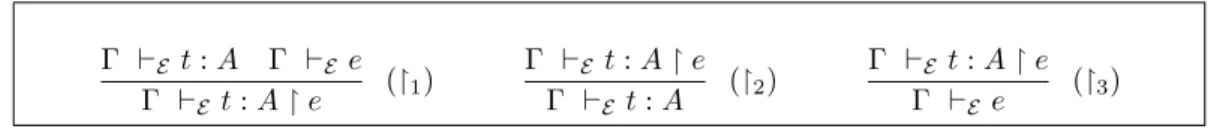
Furthermore, for the sake of presentation we do not state all the rules (which also include those ofAF2), but only give those needed for our purpose.
Γ ⊢E t:A Γ ⊢E e
Γ ⊢E t:A↾e
(↾1) Γ ⊢E t:A ↾e
Γ ⊢E t:A
(↾2) Γ ⊢E t:A ↾e
Γ ⊢E e
(↾3)
Table 2: Rules of the hiding operator↾.
The hiding operator is used with a relation≺where the definition of formulas given in section 2.1 is now completed as follows:
IfAis a formula, andu, v are terms thenA↾(u≺v) is a formula.
If A is a formula where a distinguished variable x occurs, we abbreviate the formula
A[u/x]↾(u≺v) with the notationAu≺v.
Among the rules of TTR, several rules are used to reproduce, from the programming point of view, the reasoning by induction. The rule below stands in TTR for an external induction rule where the relation≺denotes a well-founded partial ordering on the terms of the algebra:
Γ⊢E t:∀x[∀z[Dz≺x→B[z/x]]→[D(x)→B]]
Γ ⊢E (T t) :∀x[D(x)→B] (Ext)
In the rule (Ext), the lambda term T is the Turing fixed-point operator,D is a data type andxis a variable not occurring in the formulaB.
From the (Ext) rule, it is possible to derive theIndg formula: g
Ind:=∀x(Dr(x)→ ∀X(∀y(Dr(y)→ ∀z(Drz
≺y→X(z))→X(y))→X(x))).
That is, for each recursive data type, there is aλ-termindsuch that: ⊢E ind:Indg for
any setE of equations. We say that the termindwitnesses the proof ofIndg. This is stated with Lemma 2.1 below, which is presented with the type of natural numbers in [15].
Lemma 2.1. For each recursive data type, there exists aλ-termindsuch that:
⊢E ind:Indg for any setE of equations.
Lemma 2.1 can be proven for E being empty. Then, one can use the result of [7] which states that if E1 ⊆ E2 then ⊢E1 t : P implies ⊢E2 t : P. The proof of Lemma 2.1 in [15],
given only with the type of natural numbers, can actually also be applied to any data type. In particular if T is the Turing fixed-point operator, then the lambda term ind = (T λxλyλz((z y)λm((x m)z))), is valid for any data type D. The above Lemma is useful for the definition of a macro-rule, called theInd-rule, in theProPre system.
2.3
The
ProPre
system
We assume that the set of functions F is divided into two disjoint sets, the set Fc of
constructor symbols and the set Fd of defined function symbols also called defined
func-tions. Each function f is supposed to have a type denoted by D1, . . . , Dn → D where
D1, . . . , Dn, D denote data symbols and n denotes the arity of the function f. We may
writef :D1, . . . , Dn →D to both introduce a functionf and its typeD1, . . . , Dn→D.
• AspecificationEf of a defined functionf :D1, . . . , Dn →DinFd is a non overlapping
set of left-linear equations{(e1, e′1), . . . ,(ep, e′p)}such that for all 1≤i≤p,eiis of the
formf(t1, . . . , tn) where tj is a constructor term (i.e. without occurrences of defined
function symbols) of typeDj,j= 1, . . . , n,ande′i is a term of typeD.
• Thetermination statementof a functionf :D1, . . . , Dn→Dis the formula
∀x1(D1(x1)→. . .→ ∀xn(Dn(xn)→D(f(x1, . . . , xn)))).
• LetEf a specification of a functionf. Arecursive calloff is a pair (t, v) wheretis the
left-hand side of an equation (t, u) ofEfandva subterm ofuof the formf(v1, . . . , vn).
An equation (l, r) of a specification may be written l = r (as an equational axiom in TTR). We may also drop the brackets to ease the readability.
The formal proofs ofProPre, called I-proofs, are built upon distributing trees, based on two main rules derived from theTTRStructrule and theIndrule in [12]. The distributing trees built in ProPreare characterized by a property calledformal terminal state property. This section presents these two main rules, the distributing trees and the formal terminal state property. Let us first introduce some notations.
Notation 2.3. IfPis the formulaF1, . . . , Fk,∀xD′(x), Fk+1, . . . , Fm→D(t), thenP−D′(x),
will denote the formulaF1, . . . , Fk, Fk+1, . . . , Fm→D(t).
The above notation is correct as it will be used at the same time when the quantified variablexwill be substituted by a term in the formulaP−D(x) with respect to the context
(cf. next two lemmas with Notation 2.4) or when the variablex will be introduced in the context.
Notation 2.4. LetCbe a constructor symbol of a typeD1, . . . , Dk→D. Letx1, . . . , xk, z
be distinct variables. LetF(x) be a formula in which the variablexis free and the variables
z, x1, . . . , xk do not occur and lett=C(x1, . . . , xk). Then ΦC(F(x)) and ΨC(F(x)) will be
respectively the following formulas:
• ΦC(F(x)) is: ∀x1D1(x1), . . . ,∀xkDk(xk)→F[t/x];
• ΨC(F(x)) is: ∀x1D1(x1), . . . ,∀xkDk(xk),∀z(Dz≺t→F[z/x])→F[t/x].
The notation may suggest some kind of formulas that are actually useful in the construc-tion of I-proofs which are defined as follows:
Definitions 2.5. [I-formulas and restrictive hypothesis]
• A formula F is called an I-formula if and only if F is of the form H1, . . . , Hm →
D(f(t1, . . .,tn)) for some:
−data typeD, defined functionf,
−formulasHi for i= 1, . . . , m such thatHi is of the form∀xD′(x) or of the form
∀z(D′z
≺u→F′) for some data typeD′, I-formula F′ and termu.
• AnI-restrictive hypothesisof an I-formulaFof the formH1, . . . , Hm→D(f(t1, . . .,tn))
is a formulaHiof the form∀z(D′z≺u→F′). We say thatH′is arestrictive hypothesis
to an I-restrictive hypothesisH =∀z(D′z
≺u→F′) ifH′is an I-restrictive hypothesis
The definition of an I-formula is recursive, and an I-formula may have sub-I-formulas. An I-restrictive hypothesis is not an I-formula and we can use the termrestrictive hypothesis to also denote I-restrictive hypothesis. The termination statement of a defined function is an I-formula which has no restrictive hypothesis.
The lemmas below state that one can use two additional rules, calledStructrule andInd
rule, inTTRas they can be derived from the other rules ofTTR. These rules correspond to macro-rules, the former one can be seen as a reasoning by cases, while the last one stands for an induction rule.
Lemma-Definition 2.6. [The Ind rule]
LetDbe a data type and consider all the constructor functionsCiof typeDi1, . . . , Dik→D,
0 ≤ ik, i = 1, . . . , q. Let P be a formula of the form F1, . . . , Fk,∀xD(x), Fk+1, . . . , Fm →
D′(t), and Γ a context. For Ψ
Ci(P−D(x)) given as in Notation 2.4, the inductionInd rule
on type Dis:
Γ ⊢E ΨC1(P−D(x)) . . . Γ ⊢E ΨCq(P−D(x))
Γ ⊢E P
Ind(x)
Along with theIndrule, theStructrule defined below, which is also a macro-rule derived fromTTR, can be considered as a reasoning by cases.
Lemma-Definition 2.7. [The Struct rule]
LetDbe a data type and consider all the constructor functionsCiof typeDi1, . . . , Dik→D,
0 ≤ ik, i = 1, . . . , q. Let P be a formula of the form F1, . . . , Fk,∀xD(x), Fk+1, . . . , Fm →
D′(t), and Γ a context. For Φ
Ci(P−D(x)) given as in Notation 2.4, theStruct rule on type
D is:
Γ ⊢E ΦC1(P−D(x)) . . . Γ ⊢E ΦCq(P−D(x))
Γ ⊢E P
Struct(x)
Due to these lemmas, two macro-rules can be added inTTR: theStruct-rule (Lemma 2.7) and the Ind-rule (Lemma 2.6). From these rules, distributing treescan be built in ProPre
(see Definition 2.10).
Remark 2.8. I-formulas are preserved by theStruct-rule and theInd-rule. That is, ifP
is an I-formula, then so are: ΦC(P−D(x)) and ΨC(P−D(x)).
Definition 2.9. [Heart of formula] Theheartof a formula of the formF=H1, . . . , Hm→
D(t), whereD is a recursive data type, will be the termt, denoted by H(F).
The distributing trees are defined as follows:
Definition 2.10. [Distributing tree] Assume Ef is a specification of a function f :
D1, . . . , Dn → D. A is a distributing tree for Ef iff A is a proof tree built only with the
Structrule andIndrule where:
1. the root ofAis the termination statement off with the empty context, i.e.:
⊢Ef ∀x1D1(x1), ...,∀xnDn(xn)→D(f(x1, ..., xn)).
2. if L ={Γ1 ⊢Ef F1, ...,Γq ⊢Ef Fq} is the set of A’s leaves, then there exists a one to
one applicationB: L֒→ Ef such thatB(L) = (t, u) with L= (Γ⊢Ef F) in Land the
Note that it can be inductively checked, from the root, using remark 2.8, that any formula in a distributing tree is an I-formula.
The I-proofs found by theProPresystem are formal termination proofs of termination statements of defined functions. They are divided into three phases:
1. the development of a distributing tree for the specification of a defined function, char-acterized by a property, called formal terminal state property;
2. each leaf of the distributing tree is extended into a new leaf by an application of an (eq) rule;
3. each leaf, coming from the second step, is extended with a new sub-tree, with the use of rules defined in [12], whose leaves end with axiom rules.
Due to the following fact proved in [12], it is not necessary to consider in this paper the middle and upper parts of proof trees built in theProPresystem:
Fact 2.11. A distributing tree T can be (automatically) extended into a complete proof tree iffT enjoys a property, called theformal terminal state property.
That is, it is enough to look at distributing trees that have the formal terminal state property to be able to complete the proof tree and hence state the termination of the function. Therefore it remains for us to state the mentioned property.
Definition 2.12. We say that an I-formula or a restrictive hypothesisP can be applied to a term tif the heart H(P) ofP matchest according to a substitution σwhere for each variablexthat occurs free inP we have σ(x) =x.
The relation≺of Definition 2.5 deals with the measure|.|# on the terms, ranging over
natural numbers, which counts the number of subterms of a given termt (includingt), and is interpreted as follows:
Definition 2.13. LetVar(t) be the set of variables occurring int. Letu, v be terms. We say thatu≺v iff: |u|#<|v|#,Var(u)⊆ Var(v), anduis linear.
This clearly defines a well-founded ordering≺on terms. We can now state the main property that a distributing tree must enjoy in the I-proofs ofProPre.
Definition 2.14. [Formal Terminal State Property]
Let Ef be a specification of a function f and A be a distributing tree for Ef. We say
that A satisfies the formal terminal state property (ftsp) iff for all leaves L = (Γ ⊢Ef F)
of A with the equation e ∈ Ef such that B(L) = e, where B is the application given in
Definition 2.10, and for all recursive calls (t, v) of e, there exists a restrictive hypothesis
P =∀zDz≺s, H1, . . . , Hk→D(w) ofF and a substitutionσsuch thatP can be applied to
v according toσ with:
1. σ(z)≺sand
2. for all restrictive hypothesisH of P of the form∀yD′y
≺s′ →K there is a restrictive hypothesisH0ofF of the form∀yD′y≺s0 →K withσ(s
′)s 0.
So,ProPreestablishes the termination of a functionf by showing that the distributing tree of the specification of f (which is a partial tree whose root is the termination statement of
Γ⊢Ef P
❏ ❏ ❏ ❏ ❏ ❏ ❏
✡✡ ✡✡
✡✡✡
⊢Ef F
F: termination statement
Distributing Tree
H
✲ H(P)
❏ ❏ ❏ ❏ ❏ ❏ ❏
✡✡ ✡✡
✡✡✡
H(F)
Term Distributing Tree
Figure 1: The operator H
3
The abstract terminal state property
Proof structures can often be heavy and difficult to work with. However, in the constructive framework of the Curry-Howard isomorphism, compiling a recursive algorithm corresponds to establishing a formal proof of its totality. InProPre, termination proofs play an important role as they make it possible to obtain λ-terms that compute programs. We set out to simplify the termination techniques developed in ProPre by showing that its automated formal proofs can be abstracted giving rise to a simpler property which respects termination. Instead of dealing with formulas, we will use the simpler concept of functions. Also, instead of data symbols, we will use sorts and assume that there is a correspondence between the data types of ProPre and our sorts. Instead of the complex concept of distributing trees used in ProPre (Definition 2.10), we will use the much simpler notion ofterm distributing treesof [14]. By living in the easier framework, we will introduce the newabstract terminal state property which will play for term distributing trees a similar role to that played by the formal terminal state property for distributing trees. In this section we present a data structure for which we will be able to introduce a new termination property.
We consider a countable setX of individual variables and we assume that each variable of
X has a unique sort and that for each sortsthere is a countable number of variables in X
of sorts. For sorts,F subset ofF, and X subset ofX,T(F,X)s denotes the set of terms
of sortsbuilt fromF andX. In caseX is empty we will also use the notation T(F)s.
We recall the definition of term distributing trees of [14]. A term distributing tree is much simpler than the distributing tree of ProPregiven in Definition 2.10. The novelty of this section will be a term distributing tree equipped with abstract terminal state property (Definition 3.5 below).
Definition 3.1. [Term distributing tree] Let Ef be a specification of a function f :
s1, . . . , sn→s. T is a term distributing treeforEf iff it is a tree where:
1. its root is of the formf(x1, . . . , xn) wherexi is a variable of sortsi, i≤n;
2. each of its leafs is a left-hand side of an equation ofEf (up to variable renaming); and
3. each node f(t1, . . . , tn) of T admits one variable x′ of a sort s′ such that the set
of children of the node is {f(t1, . . . tn)[C(x′1, . . . x′r)/x′], where x′1, . . . , x′r are not in
t1, . . . tn andC:s′1, . . . , s′r→s′∈ Fc}.
A term distributing tree can bee seen as a skeleton form of a distributing treeT by taking the heart of the formulas in the nodes ofT, which gives rise to an operatorHillustrated by Figure 1.
Proposition 3.2. If there is a distributing tree for a specificationEf of a functionf then
there is also a term distributing tree for the specificationEf.
A term distributing tree is easier to handle than a distributing tree. But, in both parts of Figure 1, term distributing trees and distributing trees may have no termination property. However, we know by Fact 2.11 that a function terminates if we have a distributing tree that satisfies a right terminal state property. What we want is to define a notion on the term distributing trees that also ensures the termination of functions. We first give some notations and remarks.
Notations 3.3. LetT be a term distributing tree with rootθ1.
• A branchb from θ1 to a leaf θk is denoted by (θ1, y1), . . . ,(θk−1, yk−1), θk where for
eachi≤k−1,yi corresponds to the variablex′ for the nodeθi in the third clause of
Definition 3.1. We useLb to denote the leaf of the branchb.
• If a nodeθ matches a term u of a recursive call (t, u) then the substitution will be denoted byρθ,u (in particular in Definition 3.5).
• For a termtof a left-hand side of an equation,b(t) will denote the branch in the term distributing tree that leads tot(second clause of Definition 3.1).
Remarks 3.4.
• Letf :s1, . . . , sn →s be a function andEf be a specification of f. Let T be a term
distributing tree of Ef. Then for each (w1, . . . , wn) ofT(Fc)s1 ∗. . .∗ T(Fc)sn there
is one and only one leaf θ of T and a ground constructor substitution ϕ such that
ϕ(θ) =f(w1, . . . , wn).
• LetT be a term distributing tree for a specification and letb be a branch from the rootθ1 of T to a leafθk with b = (θ1, x1), . . . ,(θk−1, xk−1), θk. Then for each node
θi, θj with 1≤i≤j ≤k, there exists a constructor substitution, denotedσθj,θi, such
thatσθj,θi(θi) =θj.
Now, we give theabstract terminal state propertyfor term distributing trees:
Definition 3.5. [Abstract terminal state property]
Let T be a term distributing tree for a specification. We say that T has the abstract terminal state property (atsp) if there is an application µ :T → {0,1} on the nodes of T
such that if L is a leaf,µ(L) = 0, and for every recursive call (t, u), there is a node (θ, x) in the branch b(t) with µ(θ) = 1 such that θ matches u with ρθ,u(x) ≺ σLb(t),θ(x) (cf.
Notations 3.3 and Remark 3.4) and for all ancestors (θ′, x′) ofθ in b(t) with µ(θ′) = 1, we
have ρθ′,u(x′)σLb(t),θ′(x ′).
Note that similarly to term distributing trees, no formula is mentioned in the definition of atsp and henceatsp is easier to handle than ftsp (Definition 2.14) because atsp only uses relations of substitutions where all proposition informations have been abstracted. However, it is not obvious that a term distributing tree that satisfiesatsp implies the termination of the given function. A way to prove this fact would be to infer some particular measures from such distributing trees and to show that these measures have the decreasing property through the recursive calls of the given function so that the function terminates.
4
Building formal proofs from skeleton forms
The aim of this section is first to show that the atspcan be viewed as an abstract form of the theftsp. This is formally stated with Theorem 4.2 below. Secondly, Theorem 4.5 states that the atsp is a sufficient condition to construct a distributing tree with theftsp from a term distributing tree (skeleton form). This can be illustrated with the picture below.
Distributing trees in Formal terminal proofs
with
(skeleton)
✲
Term distributing trees
with
Formal terminal state property
Theorem 4.2
✲ ✛
Theorem 4.5
Abstract terminal state property
We start by extending the applicationH(Figure 1) into a new operatorH′ from a
distribut-ing treeA to the term distributing tree H(A) which is now equipped with an application
µ:H(A)→ {0,1} defined on the node ofH(A), so thatH′(A) will be (H(A), µ). A term
distributing tree equipped with an application µ will also be called a µ-term distributing tree.
To define the operatorH′, the applicationµis given as follows: LetAbe a distributing tree
and (Γ ⊢Ef P) be a node of A. If (Γ ⊢Ef P) is a leaf, we take µ(H(P)) = 0. If not, we
considerµ(H(P)) = 1 if the rule applied on (Γ⊢Ef P) inAis theIndrule andµ(H(P)) = 0
otherwise.
Note thatHis not injective: there is at least two distinct distributing trees Aand A′ such
that H(A) = H(A′). However, H′ is injective. Actually if we consider term distributing
trees equipped with aµ-application, thenH′ becomes bijective and the inverse operator of
H′ can be stated with the definition below.
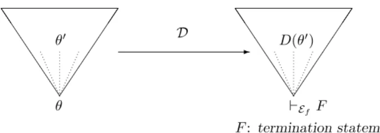
Lemma-Definition 4.1. [D, the inverse of H′] Let E
f be a specification of a function
f : s1, . . . , sn → s, and let (T, µ) be a term distributing tree for Ef (equipped with a µ
application). There is one and only one distributing treeAforEf such thatH′(A) = (T, µ).
This one can be automatically obtained from (T, µ) and we define the application Dwith
D(T, µ) =A.
Proof: LetF =∀x1D1(x1), . . . ,∀xnDn(xn)→D(f(x1, . . . , xn)) be the termination
state-ment of f. We can inductivelybuild a distributing treeA of the same size asT by taking the root ofAto be⊢Ef F and assuming the existence of a node (Γ⊢Ef P) ofA, forP is an
I-formula, such that:
i) P is of the form: F1, . . . , Fr,∀xD′(x), Fr+1, . . . , Fp → D(f(t1, . . . , tn)) where D and
D′ are data symbols, and variables in the heart ofP are bound,
ii) Tadmits a level, the same as those (Γ⊢Ef P) inA, such that the nodeθat this level is
distinct from a leaf, withθ=f(t1, . . . , tn) whose variable according to Definition 3.1.3
is the variablexof sorts′ associated toD′.
From above, we build the children nodes of (Γ⊢Ef P) inAas follows:
•Ifµ(θ) = 0, the node (Γ⊢Ef P) is extended by theStructrule onxinP.
•Ifµ(θ) = 1, the node (Γ⊢Ef P) is extended using theIndrule onxin P.
In both cases, sinceP is an I-formula, if P′
D(θ′)
❏ ❏ ❏ ❏ ❏ ❏ ❏
✡✡ ✡✡
✡✡✡
⊢Ef F
F: termination statement
Distributing Tree
D
✲
θ′
❏ ❏ ❏ ❏ ❏ ❏ ❏
✡✡ ✡✡
✡✡✡
θ
Term Distributing Tree
Figure 2: The reverse operator ofH′
Definitions 2.6 and 2.7 as a children node ofP, then P′
j is an I-formula. As the variables
that occur in P are bound, by construction of its children, the variables occurring in the heart ofP′
j are bound too. Now, due to the definitions of the term distributing trees and the
IndandStructrules, it is easy to see that there is a child nodeθj ofθsuch thatC(Pj′) =θ′j.
Therefore, the above process allows the property ii) to be held by each child of (Γ⊢Ef P)
except if the corresponding node inT is a leaf. By definition ofA, C′(A) = (T, µ) and its uniqueness results from injectivity ofC′. This gives the associated treeA=D(T) ofT with
C′(D(T, µ)) = (T, µ). Hence we deduce, because C′ is injective, thatD(C′(A)) =Afor each
distributing tree. ✷
This means that for any distributing tree A and term distributing tree (T, µ), we have:
D(H′(A)) =AandH′(D(T, µ)) = (T, µ). We can illustrateDwith Figure 2.
However there is still no warranty on the termination of functions usingµ-term distribut-ing trees. The first theorem below shows that theatspofµ-term distributing trees stands in some sense for theftsp from which all proposition informations are abstracted in a simpler context.
Theorem 4.2. LetEf be a specification of a function f andA be a distributing tree for
Ef. IfAhas the formal terminal state property then the term distributing tree H′(A) has
the abstract terminal state property.
Proof: Similar to the proof of Theorem 4.5 below. ✷ Before giving the opposite of Theorem 4.2, Theorem 4.5, we need to introduce the following two definitions:
Definition 4.3. [Nr(Q, P)] Let P be an I-formula and Q a restrictive hypothesis of P.
Nr(Q, P) is the number of restrictive hypotheses ofP that appear between the outermost
restrictive hypothesis of P. E.g., if Q is the outermost restrictive hypothesis of P, then
Nr(Q, P) = 1. Ni(P) is the number of restrictive hypothesis ofP.
Definition 4.4. [T rj,kb (Q)] Let A be a distributing tree for a specification Ef. Let b be
a branch and P a node in b at a level i from the root. We define T rbi+1,i(Q), where Qis
a restrictive hypothesis of P, as the restrictive hypothesisQ′ in the child P′ of P in b as
follows depending on whether the rule applied onP is:
• Struct: Q′ is the restrictive hypothesis whereN
r(Q′, P′) =Nr(Q, P).
• Ind: Q′ is such thatN
We also define T rbj,k(Q) with j > k as the restrictive hypothesis of the nodeP′′ at levelj
in bdefined by: T rj,kb (Q) =T rj,jb −1◦. . .◦T rbk+2,k+1◦T rbk+1,k(Q). FinallyT ri,ib will denote the identity onP.
The next theorem is the opposite of Theorem 4.2 and shows that we can automatically rebuild a distributing tree that has the ftsp from a skeleton form that has the atsp. As a consequence, according to Section 2.3, we can also build an I-proof and thus extract a
λ-term that computes the given function.
Theorem 4.5. LetEf be a specification of a functionf and (T, µ) be aµ-term distributing
tree for Ef. If (T, µ) has the abstract terminal state property then the distributing tree
D(T, µ) has the formal terminal state property.
Proof: Let (T, µ) be a term distributing tree forEf which has theAtsp. We want to show
thatD(T, µ) has theftsp. Take a recursive call (t, v) of an equation ofEf. We have to find a
restrictive hypothesisR =∀zDz≺s, F1, . . . , Fk →D(w) inLof D(T, µ) with B(L) = (t, v),
whereB is the application of Definition 2.10, such that clauses 1. and 2. of Definition 2.14 hold. LetB be the corresponding branch inD(T, µ) ofb(t) in T, and let (θ, x) be the node in b(t) given in Definition 3.5. Consider (Γ⊢Ef P) in D(T, µ) that is at the same level of
(θ, x) inT. Asµ(θ) = 1, by construction ofD(T, µ), a new restrictive hypothesis of the form
Q=∀z(Dz≺s→P−D(x)[z/x]) is created in the childP′ ofP in B. ConsiderR=T rBj,i(Q)
the restrictive hypothesis in Bwhere iandj are respectively the level ofP′ and the leaf of
B. We can writeR=∀z(Dz≺s′ →P−D(x)[z/x]) for some terms′ because:
1) The free variables inQ are those of the term s, and the appliedInd/Struct rule is done on a variable inP′ which is out of the scope ofQ.
2) As 1) first holds forQ′=T ri+1,i
B (Q), next holds for T r i+2,i B (Q)=T r
i+2,i+1
B (Q′), . . . , we
have that: R=T rj,iB(Q) =∀z(Dz≺s′ →P−D(x)[z/x]) where the variables ofC(R) are closed inR.
Clause 1 We know thatθ matchesv with a substitutionρθ,v, butC(P) =θ, so Rcan be
applied tovaccording to a substitutionσdefined withσ(z) =ρθ,v(x) andσ(y) =ρθ,v(y) for
y 6=z. We have to show thatσ(z)≺s′. This can be easily proved, by induction onk≥i,
that if T rBk,i(Q) =∀z(Dz≺sk →P−D(x)[z/x]) for some term sk, thensk =σk,i−1(x) where
the node θ matches the node at levelkin T with the substitution σk,i−1. By definition of
j, σj,i−1 = σLB,θ, so ρθ,v(x) ≺ σj,i−1(x) by Definition 3.5, and we can now deduce that
σ(z)≺s′ sinces′ =s
j. Therefore clause 1. of Definition 2.14 holds.
Clause 2 Consider a restrictive hypothesis H =∀zD′z
≺r → K in R; we have to find a
restrictive hypothesis H0 in P of the form ∀zD′z≺r0 → K such that σ(r) r0. As H is
a restrictive hypothesis of T rj,iB(Q), H is also a restrictive hypothesis of Q. Hence, one
associates toH a restrictive hypothesisH′ in
P′ =∀x
i1Di1(xi1), . . . ,∀xikDik(xik),∀z(Dz≺si →P−D(x)[z/x])
| {z }
Q
→P−D(x)[si/x],
where H and H′ respectively appear in P
−D(x)[z/x] andP−D(x)[si/x]. As H is of the
form ∀zD′z
≺r →K thenH′ is of the form ∀zD′z≺r0 →K since only the variables in the
term r are free in H. Now consider the node (Γ ⊢Ef N) in B at a level l such that 1)
a new restrictive hypothesis M is created in the child N′ of N in B, namely, N
i(N′) =
Ni(N) + 1 and Nr(M, N′) = 1, and 2)T ri,lB(M) = H′. Let (θ′, x′) be the corresponding
node in T of (Γ ⊢Ef N) in A. It is clear that θ
′ is an ancestor of θ in T since l < j
we have the relation ρθ′,v(x′) σLb(t),θ′(x
′). Let us now choose H
0 =T rj,lB+1(M) as the
restrictive hypothesis in P′. Using the same property of clause 1 as we did withT rj,iB(Q),
we know that r0 is σj,l(x′) = σLb(t),θ′(x
′). Let us show that σ(r) = σ
θ′,v(x′). We note
that i−1≥l+ 1 sincei−1 andl are respectively the level of P andN that are distinct. We have T riB−1,l+1(M) = ∀z(D′z
≺σi−1,l(x′) → K) in P, where σi−1,l is by definition the
substitution σθ,θ′. So, according to the restrictive hypothesis Q in P′, the term r in H is σθ,θ′(x′)[z/x]. Now, by definition of σ in clause 1 of Definition 2.14, we have σ(r) =
ρθ,v{z→x}(σθ,θ′(x′)[z/x]) = ρθ,v(σθ,θ′(x′)). But the relation of substitutions gives usρθ′,v=
ρθ,v◦σθ,θ′. So we finally obtainσ(r) = ρθ′,v(x′), and we can deduce from the above and
Definition 3.5 thatσ(r)r0. Hence, clause 2. of Definition 2.14 holds. ✷
In [5], measures were related to given functions whose decreasing property through the recursive calls were dependent on theftspenjoyed by distributing trees. We claim that it is possible to infer measures directly from term distributing trees whose decreasing property through the recursive calls of the considered functions now rely only onatsp. We do not state the measures for lack of space but just remark that this is a straightforward consequence of the results of this section with the previous one and [5].
Following distributing tree withatsp makes the analysis of the I-proofs easier. In par-ticular there are no measures from [5] associated to thequot function (defined in the next section) that have the decreasing property (see [4]). As a consequence of the above results of this section, there are no I-proofs for such function. The aim of the following section is to show that the framework ofProPre can actually be applied to new functions (e.g. quot
function) provided an automated termination procedure (e.g. [4, 1, 2]) is used.
5
Synthesizing programs from termination techniques
As noted in Section 2, if we can prove, in TTR, a formula that states the totality of a function then it is possible, in term of programs, to obtain a λ-term as the code of the function. As earlier mentioned, this formula is calledtermination statementinProPre (Def-inition 2.2). More precisely, assume thatEf1, . . . ,Efm are specifications of defined functions
already proved in theProPre system. Letf be a new defined function with a specification
Ef. We put E = ⊔jj==1nEfj, and E
1
f = Ef ⊔ E. In order to obtain a lambda term F that
computes the new functionf,ProPreneeds to establish⊢E1
f F :Tf in TTR.
Now consider the following specification function :
Example 5.1. Letquot:nat, nat, nat→natbe a defined function with specificationEquot
given by the equations:
quot(x,0,0) = 0 quot(s(x), s(y), z) =quot(x, y, z)
quot(0, s(y), z) = 0 quot(x,0, s(z)) =s(quot(x, s(z), s(z))
The valuequot(x, y, z) corresponds to 1 +⌊x−y
z ⌋when z6= 0 and y≤x, that is to say
quot(x, y, y) computes ⌊x
y⌋. Its specification does not admit an I-proof and therefore no
λ-term can be associated by theProPresystem.
To circumvent this drawback, we show, considering the framework ofProPreandTTR, that it is possible to add other automated termination procedures than the one ofProPre
regarding the automation of the extraction ofλ-terms.
A new relation≺
Formal Proof of Totality of ˜f
Termination Proof off given with an automated procedure
Product Types ✛
✲
Lemma 5.4 Formal Proof of Totality off
Figure 3: A formal proof of totality of the functionf.
algorithm designed in ProPre. Said informally, to convey the termination informations in the formal proof inProPre, it is used with the relation≺included in formulas of the form
A[u/x]↾(u≺v) due to Table 2.
Now assume, for a given function that terminates, the equations admit only one argu-ment. This provides a natural (partial) relation on the data type on which the function is specified so that each recursive call decreases. Also assume that an automated procedure ensures the termination of this function. Then this one can be used as the termination al-gorithm ofProPre, but we now consider the new relation instead of the earlier relation≺of
ProPre. Due to the hiding rules of the operator↾we can develop a particular formal proof, as an I-Proof, for the considered function but where in particular the sequent Γ⊢E(u≺v)
in the rule (↾1) withe= (u≺v) can be obtained with the new termination procedure that
provides the new relation ≺.
In case the function admits several arguments, we would like to cluster the arguments of the equations of the specification into one argument. To do so, we show that the use of uncurryfication forms of functions is harmless in TTR (also inAF2) in the sense given by Lemma 5.4 by considering the product types. As a consequence this enables us to follow the principle illustrated in Figure 3 where ˜f stands for an uncurryfication form of a given functionf. The left part of Figure 3 is obtained with Theorem 5.7.
We will now come into more details to get the synthesis of a function concerning the above principle.
5.1
Product types
We introduce particular specifications that correspond in some sense to uncurryfication forms of earlier specifications. To do so, we will consider a product type associated to a function. As we have not stated the data types of TTR with the operatorµ(cf. beginning of Section 2.2), for the sake of presentation, we present below the product types in the context ofAF2. This presentation in Definition 5.2 is harmless because Lemma 5.4 below and its proof hold both inAF2 andTTR.
Definition 5.2. [Product type of a function]
Letf :D1, . . . , Dn→D be a defined function,cp∈ Fc be a new constructor of aritynand
take the termination statement off:
Tf =∀x1. . .∀xn(D1(x1), . . . , Dn(xn)→D(f(x1, . . . , xn))). The data typeK(x) defined by
the formula: ∀X∀y1. . .∀ynD1(y1), . . . , Dn(yn) → X(cp(y1, . . . , yn)) → X(x) is called the
product type ofD1, . . . , Dn, and is denoted by (D1×. . .×Dn)(x).
Starting from the specification of a defined functionf it is possible to associate another defined function ˜f whose specificationEf˜takes into account the product type off.
Definition 5.3. Let f : D1, . . . , Dn → D be a defined function with a specification Ef.
Let ˜f be a new defined symbol inFd, which is called thetwin functionoff. To define the
f(t1, . . . , tn) =v ofEf wherecpis the constructor symbol of the product type associated to
f. The termv is recursively defined fromv as follows:
• (i) ifv is a variable or a constant thenv=v,
• (ii) if v =g(u1, . . . , um) with g a constructor or a symbol function distinct from f,
thenv=g(u1, . . . , um),
• (iii) ifv=f(u1, . . . , un) thenv= ˜f(cp(u1, . . . , un)).
Note that this clearly defines the specification Ef˜of the defined function ˜f associated tof,
and that the termination statement of ˜f is:
Tf˜=∀x((D1×. . .×Dn)(x)→D( ˜f(x))).
Let us consider the specification Ef of a function and the set of equations Ef′ = Ef∪
{f(x1, . . . , xn) = ˜f(cp(x1, . . . , xn))}. The set Ef′ is not a specification according to
Defini-tion 2.2 inProPre, but we can still reason inTTR. Assume the termination statement of ˜f
proved inTTRwithEf˜and the setE of the specifications already proved. Now we can add
the equations of Ef˜in the setE before proving the termination statement Tf. Due to the
form of the specifications Ef˜and Ef, the equation f(x1, . . . , xn) = ˜f(cp(x1, . . . , xn)) does
not add any contradiction in the set of the equational axiomsEf⊔ E. Therefore we can now
use the new set E′
f ⊔ E to prove the termination statement Tf in TTR. So, the equation
f(x1, . . . , xn) = ˜f(cp(x1, . . . , xn)) provides the connection betweenEf and Ef˜from the
log-ical point of view and the proof ofTf˜provides the computational aspect of the functionf.
More precisely we have the following lemma.
Lemma 5.4. Letf :D1, . . . , Dn→Dbe a defined function with a specificationEf, andEf˜
the specification of the twin function ˜f. LetE1, . . . ,En be the specifications of the defined
functions already proved (in AF2 or TTR), E = ⊔i=n
i=1Ei. Let us note Ef1˜ = Ef˜⊔ E and
E2 ˜
f =E
′ ˜
f⊔ E
1 ˜
f with E
′
f = Ef ∪ {f(x1, . . . , xn) = ˜f(cp(x1, . . . , xn))}. If there is aλ-term Fe
such that⊢E1 ˜
f
e
F :Tf˜, then there is aλ-termF such that⊢E2 ˜
f F :Tf.
Proof: This lemma holds both in AF2 andTTR, (using the rules in Table 1). We assume familiarity withAF2 and only give steps without naming the rules. LetK= (D1×. . .×Dn)
be the product type of f with cp the associated constructor symbol. By definition of the data typeK, we get inTTR:
a1 :D1(x1), . . . , an:Dn(xn)⊢Efλk(. . .((k a1)a2). . . an) :K(cp(x1, . . . , xn)).
Hence: a1:D1(x1), . . . , an:Dn(xn)⊢E1 ˜
f
(F λke (. . .((k a1)a2). . . an)) :D( ˜f(cp(x1, . . . , xn))).
BecauseE1 ˜
f ⊂ E
2 ˜
f we have:
a1 :D1(x1), . . . , an:Dn(xn)⊢E2 ˜
f
(F λke (. . .((k a1)a2). . . an)) :D( ˜f(cp(x1, . . . , xn))).
Now, we have the equation f(t1, . . . , tm) = ˜f(cp(t1, . . . , tm)) inEf2˜.
Hence: a1:D1(x1), . . . , an:Dn(xn)⊢E2˜
f( e
F λk(. . .((k a1)a2). . . an)) :D(f(x1, . . . , xn)).
Finally: ⊢E2 ˜
f F :Tf, withF =λa1. . . λan(
e
F λk(. . .((k a1)a2). . . an)). ✷
5.2
Canonical I-proofs
Letf :D1, . . . , Dn→Dbe a defined function, with a specificationEf, which is terminating
with an automated procedure. As mentioned earlier, instead of using the ordering of the terms given in Definition 2.13, we define a new ordering for the symbol relation ≺ by considering the ordering given with the recursive calls of the equations of the specificationEf˜.
As in theProPresystem, we will assume that we have a subsetF⋆
d ofFdof defined functions
whose specification admits a proof of totality inTTR (the functions already introduced by the user) so that the defined functions occurring in the specification of the function f for which we want to prove the termination statement, are inF⋆
d ∪ {f}.
Now, let t be a term in T(F,X)s′, for some sort s′ (see Section 3), such that all the defined functions occurring in t admit a specification and are terminating. Then, for each ground sorted substitutionσ, we can define the ground termppσ(t)qqas the term inT(Fc)s
that corresponds to the normal form ofσ(t). The definition ofppσ(t)qqmakes sense as the functions occurring in the specification f are terminating which gives the existence of the normal form while the definition of the specifications (Definition 2.2) gives the uniqueness of the normal form. Therefore, we can state formally the relation≺f˜below.
Definition 5.5. Let Ef˜ be a specification of the twin function of a defined function
f such that the functions occurring in the specification Ef˜ admit a specification and are
terminating. We also assume the functionf to be terminating. LetK be the product type (D1×. . .×Dn) associated tof andcpthe constructor associated toK. We define a relation
≺f˜onKsuch that for each recursive call (f(cp(t1, ..., tn)), f(cp(v1, . . . , vn))) ofEf˜, we have
cp(ppσ(v1)qq, . . . ,ppσ(vn)qq) ≺f˜ σ(cp(t1, . . . , tn)) for any ground sorted substitutionσ.
Hence, we get the straightforward but useful following fact.
Fact 5.6. The above relation≺f˜is a well-founded ordering on K.
The next theorem says that if a functionf is terminating and if we have a distributing tree for the specification Ef˜of the twin functionf, having or lacking the formal terminal
state property, it is then possible to get a new one having the ftsp. The principle mainly consists of changing, in the initial distributing tree, the Structand Ind rules in such way that we now have a new tree with ftspwhich can be called a canonical distributing tree. It means that the formal proofs we are going to build will depend on the ability of building a distributing tree whatever its properties and on the ability of showing the termination of the function.
Theorem 5.7. LetEf be a specification of a defined function f :D1, . . . , Dn →D such
that the defined symbols that occur on the right-hand side of the equations of Ef are in
F⋆
d ∪ {f}. Let A be a distributing tree for the specification Ef˜ of the twin function ˜f.
Assume the functionf is proved terminating by a termination procedure. Then there is a distributing treeA′ forE
˜
f, which can be automatically obtained fromA, that satisfies the
formal terminal state property with the relation≺f˜.
Proof: Let Ef be a specification of a defined functionf : D1, . . . , Dn → s such that the
defined symbols that occur in the right-hand side of the equations of Ef are in Fd⋆∪ {f}.
Let A be a distributing tree for the specification Ef˜ of the twin function ˜f. We assume
f is proved terminating by a termination procedure. Since we know that the function is terminating given by an automated procedure we can introduce the ordering≺f˜. From the
term distributing tree Awe can associate a new distributing tree A′ with the ordering≺ ˜
f,
A′ ❏ ❏ ❏ ❏ ❏ ❏ ❏ ✡✡ ✡✡ ✡✡✡
⊢Ef˜Tf˜
Distributing Tree forEf˜with
formal terminal state property
}
Struct Ind(x)✲ A ❏ ❏ ❏ ❏ ❏ ❏ ❏ ✡✡ ✡✡ ✡✡✡
⊢Ef˜ Termination statement of ˜f
A Distributing Tree ofEf˜
Figure 4: The canonical distributing treeA′ ofA
Note thatA′ can be built automatically fromA. We show that A′ satisfies the formal
terminal state property. The root of A′ is ⊢
Ef˜ Tf˜, with Tf˜ = ∀x(K(x) → D( ˜f(x))) the
termination statement of ˜f where K denotes the product type (D1×. . .×Dn) and cp its
associated constructor.
LetL= (Γ⊢Ef˜P) be a leaf ofA
′ande= (t, u) be the equation ofE ˜
fwithH(P) =t. Let
(t, v) be a recursive call ofe. According to the definition of a specification and a recursive call, the terms t and v are respectively of the formf(cp(t1, . . . , tn)) and f(cp(v1, . . . , vn)).
Because of the construction of the canonical distributing treeA′ that uses a particular order
of the application rulesStructandInd(also illustrated with Figure 4),P is of the form:
∀x′i1D ′
i1(x ′
i1), . . . ,∀x ′
imD
′
im(x
′
im),∀z(Kz≺cp(h1,...,hn)→K(f(z)))
→K(f(cp(h1, . . . , hn))).
As the heart ofP isH(P) =t, we havehj=tj for any 1≤j≤n.
Now, letQ be the restrictive hypothesis ∀z(Kz≺cp(t1,...,tn)→K(f(z))) of P. Let us show
that Q can be applied to the term v according to a substitution. By the definition of Q, we haveH(Q) =f(z), so we can take a substitutionσwith σ(z) =cp(v1, . . . , vn). We also
take the valueσ(y) =y for any free variabley inQ, that is any variableyin cp(t1, . . . , tn).
Hence Qcan be applied tov according to the above substitutionσ. We now have to show the two items of Definition 2.14. As we are in the conditions of Definition 5.5, we know that
cp(ppρ(v1)qq, . . . ,ppρ(vn)qq)≺f˜ ρ(cp(t1, . . . , tn)) for any ground sorted substitutionρ. But
σ(z) =cp(v1, . . . , vn), thus we get the first item. The second item becomes straightforward:
because of the form ofQ, the set of restrictive hypotheses ofQis empty. Hence, we conclude that the canonical distributing treeA′ satisfies the formal terminal state property.
✷
The next theorem (and its proof) expresses Figure 3. It tells that if we know that a functionf is terminating, and if we have already a proof of totality of each defined function that occurs in the specification off (apart fromf), and if we have a term distributing tree associated to the specification of f, then we are able to get a λ-term that computes the functionf in the sense ofTTR.
Theorem 5.8. LetEf be a specification of a defined functionf :D1, . . . , Dn→D andD
be a given distributing tree for the specificationEf such that the defined symbols that occur
on the right-hand side of the equations ofEf are inFd⋆∪ {f}. Assume the termination of
Proof: Let ˜f be the twin function off andEf˜its specification given in Definition 5.3. By
Definition 5.3, a distributing tree A associated to Ef˜can be automatically obtained from
D. Hence, with Theorem 5.7, we now have a (canonical) distributing treeA′ associated to
Ef˜ which has the ftsp with ≺f˜ as the ordering relation. As Fact 2.11 still holds with the
new ordering relation, we get an I-proof of Ef˜that can be calledcanonical proof. Thus we
obtain a formal proof of the termination statement Tf˜in TTR. Hence, by Lemma 5.4 we
finally obtain a proof of totality off in TTR. ✷
Let us now go back to Example 5.1. It was shown in [1, 4] that the termination of the specification Equot can be proven with automated termination methods. So if we consider
such methods in the right upper part of Figure 3, we then obtain a new ordering relation
≺for the specificationEquotg of the associated functionquotg. Together with our setting, this provides a formal proof of totality ofquotg as expressed in the left part of Figure 3. Finally, using this latter result, and thanks to Lemma 5.4, we obtain a formal proof of totality of the functionquot which was not previously possible in the ProPre system .
6
Conclusion
An important part of the programming paradigms using logics as is done inProPre, is the Curry-Howard isomorphism where a λ-term is extracted from the proof. However because of the logical framework, it is often difficult to make use of termination techniques from different areas. The study of this paper has shown that, for the automated systemProPre, the extraction part of λ-terms can be released from the termination analysis, using the setting of ProPre, so that other automated termination techniques (like those of [1, 2, 4]) can now be included in this framework modulo distributing trees.
References
[1] T. Arts and J. Giesl. Automatically proving termination where simplification orderings fail. In Proceedings of Theory and Practice of Software Development TAPSOFT’97, volume 1214 ofLNCS, pages 261–272, 1997.
[2] J. Giesl. Termination of nested and mutually recursive algorithms. J. of Automated Reasoning, 19:1–29, 1997.
[3] W. A. Howard. The formulæ-as types notion of construction. In J. Hindley and J. Seldin, editors, To H.B. Curry: Essays on combinatory logic, lambda-calculus and formalism, pages 479–490. Academic Press, 1980.
[4] F. Kamareddine and F. Monin. On automating inductive and non-inductive termination methods. InProceedings of the 5th Asian Computing Science Conference, volume 1742 ofLNCS, pages 177–189, 1999.
[5] F. Kamareddine and F. Monin. On formalised proofs of termination of recursive func-tions. InProceedings of the Int. Conf. on Principles and Practice of Declarative Pro-gramming, volume 1702 ofLNCS, pages 29–46, 1999.
[7] J. L. Krivine.Lambda-calculus, Types and Models. Computers and Their Applications. Ellis Horwood, 1993.
[8] J. L. Krivine and M. Parigot. Programming with proofs. J. Inf. Process Cybern, 26(3):149–167, 1990.
[9] D. Leivant. Typing and computational properties of lambda expression. Theoretical Computer Science, 44:51–68, 1986.
[10] P. Manoury. A user’s friendly syntax to define recursive functions as typed lambda-terms. In Proceedings of Type for Proofs and Programs TYPES’94, volume 996 of LNCS, pages 83–100, 1994.
[11] P. Manoury, M. Parigot, and M. Simonot. ProPre, a programming language with proofs. InProceedings of Logic Programming and Automated Reasoning, volume 624 ofLNCS, pages 484–486, 1992.
[12] P. Manoury and M. Simonot. Des preuves de totalit´e de fonctions comme synth`ese de programmes. PhD thesis, University Paris 7, 1992.
[13] P. Manoury and M. Simonot. Automatizing termination proofs of recursively defined functions. Theoretical Computer Science, 135(2):319–343, 1994.
[14] F. Monin and M. Simonot. An ordinal measure based procedure for termination of functions. Theoretical Computer Science, 254(1-2):63–94, 2001.
[15] M. Parigot. Recursive programming with proofs: a second type theory. InProceedings of the European Symposium on Programming ESOP’88, volume 300 of LNCS, pages 145–159, 1988.