* Corresponding author:
E-mail: lenask@gmail.com
Received: June 4, 2017
Approved: November 17, 2017
How to cite: Pinheiro HSK, Carvalho Júnior W, Chagas CS, Anjos LHC, Owens PR. Prediction of topsoil texture through regression trees and multiple linear regressions. Rev Bras Cienc Solo. 2018;42:e0170167.
https://doi.org/10.1590/18069657rbcs20170167
Copyright: This is an open-access article distributed under the terms of the Creative Commons Attribution License, which permits unrestricted use, distribution, and reproduction in any medium, provided that the original author and source are credited.
Prediction of Topsoil Texture
Through Regression Trees and
Multiple Linear Regressions
Helena Saraiva Koenow Pinheiro(1)*
, Waldir de Carvalho Junior(2)
, César da Silva Chagas(2)
, Lúcia Helena Cunha dos Anjos(1)
and Phillip Ray Owens(3)
(1)
Universidade Federal Rural do Rio de Janeiro, Departamento de Solos, Seropédica, Rio de Janeiro, Brasil. (2)
Empresa Brasileira de Pesquisa Agropecuária, Embrapa Solos, Rio de Janeiro, Rio de Janeiro, Brasil. (3)
United States Department of Agriculture, Dale Bumpers Small Farms Research Center, Booneville, Arkansas, United States of America.
ABSTRACT: Users of soil survey products are mostly interested in understanding how soil
properties vary in space and time. The aim of digital soil mapping (DSM) is to represent the spatial variability of soil properties quantitatively to support decision-making. The goal of this study is to evaluate DSM techniques (Regression Trees - RT and Multiple Linear Regressions - MLR) and the ability of these tools to predict mineral fraction content under a wide variability of landscapes. The study site was the entire Guapi-Macacu watershed (1,250.78 km²) in the state of Rio de Janeiro in the Southeast region of Brazil. Terrain attributes and remote sensing data (with 30 m of spatial resolution) were used to represent landscape co-variables selected as an input in predictive models in order to develop the explanatory variables. The selection of sampling sites was based on the Latin Hypercube algorithm. A representative set of one hundred points with feasible field access was chosen. Different input databases were tested for prediction of mineral fraction content (harmonized and original data). The Spline algorithm was used to harmonize data according to the GlobalSoil.Net consortium standards. The results showed better performance from the RT models, using input from an average of six covariates; the simplest MLR model used twice as many input variables, creating more complex models without gaining precision. Furthermore, better R² values were obtained using RT models, irrespective of harmonization of soil data. The harmonized dataset from the 0.00-0.05 and 0.05-0.15 m layers, in general, presented better results for the clay and silt, with R2 values of 0.52 (0.00-0.05 m) and 0.69 (0.05-0.15 m), respectively. Prediction of sand content showed better results when the original depth data was used as an input, although all regression tree models had R2 values greater than 0.52. The RT models provided a better statistical index than MLR for all predicted properties; however, the variance between models suggests similarity of performance. Regarding harmonization of soil data, both input databases (harmonized or not) can be used to predict soil properties, since the variance of model performance was low and generalization of the soil maps showed similar trends. The products obtained from the digital soil mapping approach make it possible to integrate the factor of uncertainties, providing easier interpretation for soil management and land use decisions.
Keywords: terrain attributes, soil depth functions, digital soil mapping, regression models.
INTRODUCTION
Soil maps are widely used as primary information in land management and protection of natural resources. Soil scientists face great challenges in meeting societal demand for soil information on appropriate scales to support decisions regarding land use and management of natural resources. Digital soil mapping techniques are able to provide useful soil information on an appropriate scale and in digital format.
Soil texture or mineral particle size is a highly variable soil physical property, and studies on a regional and local scale have shown spatial dependence at short distances interfering in crops yield (Marques Júnior and Lepsch, 2000), which indicates the essential role of this property in growing crops, engineering projects, and land protection and conservation (White, 2006). The effects of soil texture on land capability, water and nutrient storage, and vegetation distribution and composition are well known globally (Klingebiel, 1963; Jenny, 1980; Silver et al., 2000; Fernandez-Illescas et al., 2001). Particle size distribution in soils is directly related to topographic indexes and slope (Leão et al., 2010, 2011).
Accurate prediction of soil texture is very important for agronomical purposes, particularly in precision farming, since soil texture is directly related to yield (He et al., 2013; Gozdowski et al., 2014). In this context, pedometric tools can be useful in predicting soil properties variability (spatial and vertical), such as soil particle size (Moore et al., 1993; Arrouays et al., 1995; McBratney et al., 2000). Usually, soil sampling at various depth intervals and description of horizons/layers are performed according to morphological properties related to pedogenesis. The measured values of soil properties correspond to the depth of the horizon, which varies according to the type of soil profile. However, surveys with specific objectives usually sample the soil according to predefined depths.
The global soil survey consortium (GlobalSoilMap project) has proposed standard depths (vertical soil profile) to expand the database of soil properties. The six pre-defined depths correspond to the following layers: 0.00-0.05, 0.05-0.15, 0.15-0.30, 0.30-0.60, 0.60-1.00, and 1.00-2.00 m. The specifications of the GlobalSoilMap project suggest that data at these six depth intervals can be harmonized through soil depth function, usually applying the equal-area quadratic spline (Arrouays et al., 2014). The legacy dataset has been successfully harmonized by Nussbaum et al. (2018), allowing comparison between different models applied to predict soil properties for distinct soil layers.
Spatial prediction of soil properties using statistical tools and pedometric concepts is supported by correlation with landscape attributes derived from a digital elevation model (DEM) and remote sensing data (Dobos et al., 2000; McBratney et al., 2003). Application of these techniques was exemplified at Moore et al. (1993), McBratney et al. (2003), and Odeh et al. (1994). Most papers concerning prediction of soil properties focus on carbon storage and hydrological properties. Multivariate linear regression models and/or tree-based models applied to predict soil properties are exemplified by Moore et al. (1993), Henderson et al. (2005), Eldeiry and Garcia (2008), Vasques et al. (2008), Ließ et al. (2012), Minasny et al. (2013), and Carvalho Junior et al. (2014a).
The study hypothesis is based that the application of digital mapping techniques can aid the quantitative spatial prediction of soil particle size components at distinct depths. In this sense, the main goal of this study was to compare two different models used to predict the spatial distribution of soil mineral particle-size fractions (clay, silt, and sand).
MATERIALS AND METHODS
Study area and soil sampling
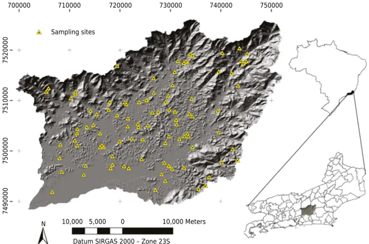
and land use by the National Policy on Water Resources (Law No, 9433/97). The Guapi-Macacu watershed is one of twelve in the Guanabara Bay Hydrographic Region. It has a catchment area of 1,250.78 km² and a perimeter of 199.2 km. The climate is classified as tropical rainy with a dry winter (Aw, according to the Köppen classification system), supporting different land uses, such as agriculture, cattle raising, and a preserved natural park under typical rainforest vegetation (Atlantic Forest). The area is located between the UTM coordinates 7488481-7526005 mS and 699292-752193 mW (horizontal datum WGS-84), and it has a wide variety of landscape features. The region is located in the central part of Guanabara Graben, known as the Macacu Sedimentary Basin, which was formed by several deposition sequences from tectonic events at the beginning of the Tertiary (Ferrari, 2001). As an example of landscape variability, elevation varies from sea level (0 m) up to 2,600 m within the watershed (Hora et al., 2010). The study was conducted in 2010 and 2011, and figure 1 shows the location of sampling sites in the Guapi-Macacu watershed in Rio de Janeiro, Brazil.
Conditioned Latin Hypercube Sampling (cLHS) was used to best achieve distribution of the sampling sites according to landscape attributes while considering the feasibility of acquiring the samples (Minasny and McBratney, 2006; Roudier et al., 2012). To set the parameters for conditioning the sampling scheme, a buffer size of 100 m to each side of the mapped roads (source: national database in scale 1:50,000 from Brazilian Institute of Geography and Statistics - IBGE), the number of sample points (100), correlation and data weight (0.5 and 1.0, respectively), and number of iterations (20,000) were set. All of these input parameters are required, and the values can be adjusted based on the specific research area and limitations (Minasny and McBratney, 2006). The selection of sampling points within this watershed was based on the parameters of spatial position, elevation slope, curvature, and land use map (Fidalgo et al., 2008). The urbanized areas were excluded, and selection of sampling sites was restricted to the buffer area (Roudier et al., 2012) defined by preliminary analyses (Carvalho Junior et al., 2014b).
10,000 Meters
Datum SIRGAS 2000 – Zone 23S 10,000
N
Sampling sites
700000 710000 720000 730000 740000 750000
5,000 0
7490000
7500000
7510000
7520000
Sand, silt, and clay content were obtained according to the procedures described by Claessen et al. (1997). The analytical results of the mineral fraction content correspond to the depth of the genetic horizons/layers, as identified in the field soil survey. The soil was classified according to the Brazilian System of Soil Classification - SiBCS (Santos et al., 2013) and the corresponding classes in the World Reference Base for Soil Resources - WRB (WRB, 2014). The typical classes that occur in the area are Planosols (Planossolos), Cambisols (Cambissolos), Gleysols (Gleissolos), Ferralsols (Latossolos), Fluvisols, and Regosols (Neossolos Flúvicos and Litólicos, respectively).
Input covariates
The main Geographic Information System (GIS) used was ArcGIS Desktop v.10 (ESRI, 2010). Terrain attributes were obtained through the System for Automated Geoscientific Analyses - SAGA v.2.1.4 (Conrad, 2007). This software is focused on landscape analysis but can be used for soil mapping (Conrad, 2007; Hengl, 2009).
Additional analyses related to remote sensing data were performed on Erdas Imagine v.9.1. software (Erdas Systems, 2008), and the landform map was created on the Geographic Resources Analysis Support System (Grass, 2013), with the Geomorphons add-on. The DEM was generated by interpolation of the primary elevation data and the drainage network, and was restricted to the watershed limits. The primary elevation data involved contour lines and precision elevation points extracted from the official Brazilian charts, 1:50,000 scale (Brazilian Institute of Geography and Statistics, and Brazilian Geological Service). An elevation model with spatial resolution of 30 m was generated by the “Topo to Raster” tool in the ArcGIS Desktop v.10. After the interpolation procedure, “sink” cells were completely filled so the final DEM would not result in interpolation failures in the model and derivatives.
Digital landscape attributes were generated from the adjusted DEM to expand the set of predictive variables used as input for the predictive models. Analyses were first performed to understand the variability of terrain variables and soil properties in the watershed. They included visual evaluation of the maps and descriptive statistics parameters (mean, standard deviation, minimum and maximum). After this procedure, thirty-seven terrain variables were selected for testing as predictor variables, as described below.
Attributes derived from the DEM and stream networks, such as elevation, slope, curvature, Compound Topographic Index (CTI), and the Euclidean distance from stream networks were generated by “Surface tools” in the “Spatial Analyst” toolbox (ArcGIS Desktop v.10). The CTI was obtained by a sequence of commands in the “grid” module of ArcINFO. These attributes were first tested, and they showed effectiveness in predicting soil classes in the same watershed (Pinheiro et al., 2013). Terrain co-variables were derived from the 30 m resolution DEM and drainage network using the “Terrain Analysis” toolbox in SAGA (System for Automated Geoscientific Analyses) to provide enough quantitative data to represent landscape features and environmental functions to predict soil properties. The derived covariates included: (i) 15 terrain attributes related to relative position and relief features [mass balance index, mid slope position, modified catchment area, multiresolution index of ridge top flatness (MrRTF), multiresolution index of valley bottom flatness (MrVBF), normalized height, protection index, slope height, valley depth, hillshade, channel network base level, altitude above the channel, vertical overland flow distance, SAGA wetness index]; and (ii) nine climatic properties (sky view factor and simplified sky view factor, solar radiation, total insolation, terrain view factor, wind effect, diffuse insolation, direct insolation, duration of insolation). Additional information about the procedures for creating terrain attributes in SAGA can be found in Olaya (2004).
add-on. The pre-defined parameters to create the landforms correspond to 45 cells (1,350 m) of search radius and 1st
of flatness threshold.
Remote sensing data from Landsat 5 TM (reference image of September/2011) were used as input variables, represented by six spectral bands (1, 2, 3, 4, 5, and 7) and three indexes calculated from the spectral bands of Landsat 5 TM, also with a 30 m spatial resolution. The indexes were the Normalized Difference Vegetation Index (NDVI), the iron oxide index (ratio between band 3/band 1), and the clay mineral index (ratio between band 5/band 7). The iron oxide index highlights the presence of iron oxides and sulfates, and the clay mineral index highlights the presence of clay minerals, such as alunite, illite, kaolinite, and montmorillonite (Sabins, 1997; Chagas et al., 2013). These last two indexes are commonly used in remote sensing applied to geology studies to recognize hydrothermal alteration and unaltered rocks (Sabins, 1999). The geology map was created by vectoring tools in ArcGIS Desktop v.10, based on the official Brazilian charts in a 1:50,000 scale (Geological Survey of Brazil and Department of Mineral Resources), and was simplified according to the type of parental material in four classes: alkaline rocks, granite/gneiss, sedimentary rocks, and quaternary sediments.
All layers were projected in the Universal Transverse Mercator (UTM) coordinate system, and the horizontal data according to the Geocentric Reference System for the Americas - Sirgas 2000, Zone 23S.
Modeling procedures
The procedures used to predict soil properties (sand, silt, and clay) were regression trees and multiple linear regression. The statistical procedures were implemented in the R software (R Development Core Team, 2014).
Multiple Linear Regressions (MLR) have been widely used to predict the response of a dependent variable from a set of independent variables, as a function of the correlations between them. The MLR algorithm was implemented using the lm( ) command, with stepwise (backward) analysis, fitting the model by removing variables according to confidence level (95 %). The approximation through least-squares was used to validate and constitute the best linear unbiased estimators of the regression parameters (Berry and Feldman, 1985; Vasques et al., 2008).
Regression Trees (RT) are implemented through the Recursive Partition and Regression Trees package, named “rpart” (Therneau et al., 2017), primarily based on the CART (classification and regression trees) algorithm (Breiman et al., 1984). The logic of the tree-based methods is a binary procedure, which is obtained by recursive partitioning of the dataset in two subsets. These methods are more homogeneous, based on the importance of the covariates over the data. This procedure is repeated recursively until the number of subsets reaches a minimum, or there are no gains in fitting models through further subdivisions. The pre-defined parameters were complexity parameter (cp) equal to 0.001 (default) and the model was fitted as analysis of variance (Anova) according to the least square mean error. Each partitioning tends to minimize the difference between two subgroups at each node, and subdivisions that do not improve the fitted model are pruned by cross-validation. Finally, terminal nodes represent the predictive value as the average of all measured values (Vasques et al., 2008).
Assuming that the influence of terrain variables on soil properties is markedly closer at the soil surface (Florinsky et al., 2002), and topsoil models are stronger than subsoil models (Henderson et al., 2005), this study focused on prediction of sand, silt, and clay content in the topsoil layer.
To meet the specifications of the GlobalSoilMap project (Arrouays et al., 2014), a new database was created from the original to represent the harmonized data in the 0.00-0.05 and 0.05-0.15 m layers. Harmonization of soil properties at regular depths was performed using the soil depth function to interpolate the data. The spline function proposed by Ponce-Hernandez et al. (1986) represents a nonparametric function, called an equal-area spline, appropriated to model soil properties (Bishop et al., 2009; Malone et al., 2009). The equal-area spline function considers each horizon as the pre-defined interval and the knots of each horizon lie between horizon boundaries, with one inflexion in each interval. The knots should lie as near as possible to the inflexion and as far from boundaries as possible, which, in essence, preserves the mean value of the soil property (Odgers et al., 2012). The spline functions were applied from the original data collected in the horizon layer (genetic horizons) to harmonize at six pre-defined depths according to the GlobalSoilMap project. From the output data generated by this procedure, the data from the first two layers (0.00-0.05 and 0.05-0.15 m) were selected to represent the topsoil layer. This procedure was performed to contrast the results obtained by the different input databases (harmonized data at two depths, and original data).
Maps and graphs were generated to compare performance between models (multivariate linear regressions and regression trees), and between input data (original depth and harmonized at 0.00-0.05 and 0.05-0.15 m). The results were compared through the coefficient of determination (R2), root mean square error (RMSE), complexity of the model (number of variables used), and map generalization. All statistical procedures used to create the maps and graphs were created on R and RStudio software, and the final layout was built with the support of ArcGIS Desktop v.10.
RESULTS AND DISCUSSION
Landscape covariates and importance in predicting soil texture
A brief description of the covariates and their respective importance in modelling the variability of soil texture in accordance with the methods tested are presented in table 1.
The predictive models (MLR and RT) tend to prioritize input variables that provide significant explanatory effects (Faraway, 2002). Redundant predictors act as noise to the estimation and should be removed to make the model as simple as possible, according to the principle of Occam’s razor, which advocates that the simplest theory should be chosen from among all theories (Young et al., 1996).
According to table 1, all models included at least one input covariate from remote sensing data (Landsat bands or derived indexes) to predict the soil properties of interest. The geology map was selected by all MLR models, regardless of the input dataset (original or harmonized), showing the direct relationship between parental material and soil texture. On the other hand, some of the terrain attributes, such as elevation, geomorphons, CTI, mass balance index, wind effect, and direction and duration of insolation, were not selected by any model tested in this study. One possible explanation is that the models discard variables correlated with each other, as highlighted by Beven and Binley (1992) and Deng et al. (2008). For example, a pairs of terrain attributes can vary simultaneously such as elevation and slope, insolation attributes, and analytical hill shading. Modified catchment area and altitude above the channel were used in one model each, showing their restricted influence on prediction of soil properties.
Table 1. Terrain attributes in the watershed: description, references, and contribution to predictive models
Covariates Description References Original data 0.00-0.05 m 0.05-0.15 m
MLR RT MLR RT MLR RT
Landsat data (band 1 to 5, 7, and indexes)
Six multispectral bands from Landsat 5 TM; derived indexes: NDVI (band 4 - band 3)/(band 4 + band 3); clay minerals (band 5/band 7); Iron Oxide
(band 3/band 1)
Yang et al. (1997), Sabins (1997, 1999), Chagas et al. (2013), Pinheiro et al. (2013)
(1,2,3) (1,2,3) (1,2,3) (1,2,3) (1,2,3) (1,2,3)
Geology map Simplified map from lithology units (Brazilian Department of Mineral
Resources, at a 1:50,000 scale)
Pinheiro et al. (2013) (1,2) N (1,2) N (1,2) N
Landform map
Landform map (Geomorphon classification) with the ten most
common landforms (flat, peak, ridge, shoulder, spur, slope, hollow, footslope, valley, and pit), considering
a broad range of scales according to the search radius distance (predefined as 45 cells) and flatness threshold (1°)
Jasiewicz and
Stepinski (2013) 0 0 0 0 0 0
Elevation
DEM from interpolation of primary elevation data, described by
Pinheiro et al. (2012)
Hutchinson and Gallant (2000), Moore et al. (1991)
0 0 0 0 0 0
Slope Slope gradient, first derivative from
the DEM (%)
Thompson et al. (2001), Wilson and
Gallant (2000)
0 (1,2) 0 (1,2) 0 (1)
Curvature classification
Classification of surface curvature based on the combination of profile and plan curvatures. Negative values
correspond to concave surfaces, positive to convex, and planar surfaces between -0.01 and 0.01
Hall and Olson, (1991), Gessler et al.
(1995), Figueiredo (2006)
(1,2,3) 0 (1,3) 0 (1,2) 0
Euclidean distance
Linear distance of the nearest stream network feature (m)
Pinheiro (2012),
Cunha (2013) (1) (1) (1) (1) (1) (1,2)
Compound topographic index - CTI
Topographic wetness index calculated according to slope and catchment area [CTI = ln (As/tan ß)], where As
is the catchment, and ß represents slope in radians
Böhner and Selige (2006), Moore
et al. (1993), Gessler et al. (1995)
0 0 0 0 0 0
Mass balance index
Represent areas of soil loss and accumulation. Negative values correspond to depressions, and positive values are related to convex
steep and erosional slopes. Values near zero represent balance between
soil loss and accumulation
Moller and Volk (2015), Moller et al.
(2008)
0 0 0 0 0 0
Mid-slope position
Relative vertical distance to the mid-slope valley or crest directions
Böhner and Antonic (2009), Häring et al.
(2012)
(3) 0 (3) 0 (3) 0
Modified catchment area
Flow accumulation in pixels as a sum of precedent flow in catchment area
(pixels or square meters)
Lea (1992), Costa‐Cabral and
Burges (1994)
0 0 0 0 0 (1)
Multiresolution index of ridge top flatness - MrRTF
Indicate flat positions on high elevation areas
Gallant and Dowling
(2003) (1,2) (2) (1,2) (2) (1,2) (2)
Multiresolution index of valley bottom flatness -MrVBF
Indicate flat surfaces on valley bottom Gallant and Dowling (2003) (1) 0 (1,2) 0 (1) 0
as a predictor covariate in all RT and MLR models. Relationships between this covariate and soil properties were observed in the field survey, particularly near the larger river basins, showing the influence of water on the genesis of soils, such as Fluvisols. These soils exhibited low clay content since the smaller particle size is easily removed from the soil profile by the action of the flow stream. This corroborates the soil map produced by
Continuation
Normalized height
Relative topographic position (%) used for modeling relative heights
and slope positions
Böhner and Conrad (2007), Nguyen et al. (2006)
(3) 0 (3) (1) 0 (3)
Protection index Maximum angle of zenith or at nadir
relating a point to surrounding relief
Yokoyama (2002), Bruna et al. (2013),
Yokoyama (2002)
(3) (1) (3) (1) (3) (1,3)
Sky view factor and Sky view factor (simplified)
Represents the fraction of visible sky viewed from the ground up. Varies from 0 to 1 from the location center
Böhner and Antonic (2009), Zakšek et al.
(2011)
(1,2,3) (1) (1,2,3) 0 (1,2,3) (1,2)
Slope height
Vertical distance from the base of the slope to the crest, or line of intersection of the two slope planes
Böhner and Conrad (2007), Gökceoglu
and Aksoy(1996)
(1,2) 0 (1,2) 0 (1,2) 0
Solar radiation
Potential incoming solar radiation (insolation) or amount of incoming
solar energy (KWH m-2
yr-1
)
Böhner and Antonic (2009), Thompson
et al. (2012)
(2,3) 0 (2,3) 0 (2,3) 0
Total insolation Sum of direct and diffuse incoming
solar radiation (KWH m-2
yr-1
)
Böhner and Antonic (2009), Wilson and
Gallant (2000)
(1,3) 0 (1,3) 0 (1,3) 0
Terrain view factor
Factor of terrain obstruction to incoming radiation
Böhner and Antonic (2009), Sandmeier
and Itten (1997)
(1,2,3) (3) (1,2,3) (2,3) (1,2,3) 0
Valley depth Vertical distance of a base level
channel network (m) Conrad (2012) (3) 0 (3) 0 (3) 0
Altitude above the channel
Vertical distance of stream network (m)
Prates et al. (2012),
Brenning (2009) 0 0 0 (2) 0 0
Vertical overland
flow distance Vertical distance projected of mean runoff length (m)
Freeman (1991), Quinn et al. (1991),
Gomi et al. (2008)
(3) 0 (2,3) 0 0 (2,3)
SAGA wetness index
Similar to the ‘Topographic Wetness Index’ (TWI); however, it is based on a
modified catchment area
Böhner et al. (2002),
Moore et al. (1993) (3) 0 (3) 0 0 (3)
Wind effect Climatic factor (m s-1)
Böhner and Antonic (2009), Ließ et al.
(2014)
0 0 0 0 0 0
Hillshading The angle between the surface and
the incoming radiation (radians) Tarini et al. (2006) 0 (2) 0 (2) 0 0
Channel network base level
Difference between the DEM and a surface interpolated from the channel
network (m)
Grimaldi et al.
(2007) (1,2,3) (3) (1,2,3) (3) (1,2,3) 0
Diffuse insolation
Incoming solar radiation reflected by atmospheric components
(KWH m-2
yr-1
)
Böhner and Antonic (2009), Wilson and
Gallant (2000)
(3) 0 (3) (1,2) (3) (1)
Direct insolation
Incoming solar insolation perpendicular to surface, excluding
diffuse insolation (KWH m-2
yr-1
)
Böhner and Antonic (2009), Wilson and
Gallant (2000)
0 0 0 0 0 0
Duration of insolation
Mean time of incoming insolation by
day (h day-1)
Böhner and Antonic (2009), Wilson and
Gallant (2000)
0 0 0 0 0 0
MLR = Multiple Linear Regression; RT = Regression Tree; NDVI = Normalized Difference Vegetation Index. (1) = Clay; (2) = Sand, (3) = Silt; 0 =
Pinheiro et al. (2017) for the same area. The terrain attributes of valley depth, normal height, and SAGA wetness index were important only for predicting silt content, which was also observed in the field, and table 1 shows each covariate used to predict the texture components. Higher silt contents were related to less developed soils, such as Regosols (Neossolos Litólicos Distróficos), Cambisols (Cambissolos Haplicos Tb Distróficos), and Fluvisols (Neossolos Flúvicos Tb Distróficos). The Fluvisols had the highest values for wetness index due to their low slopes, and their occurrence was related to deep and irregular fluvial deposits in the broader valleys. The attributes of analytical hillshade and altitude above the channel were used only in sand prediction models. Topsoil layers with high sand content were also related to proximity to river channels and young soils.
It is well known that success in modeling environmental characteristics is related to the quality of the input data, associated with a powerful set of predictive covariates (Zhu, 2001; Minasny et al., 2003). In this sense, this study can contribute to improving the modeling techniques applied to the mapping of soil properties. As for the input data, harmonization of the data allows creation of a map for the target properties corresponding to a layer of pre-defined thickness, which can be useful for agricultural purposes, for example. As for predictive covariates, by testing a large set of environmental data, it was possible to identify primarily those covariates related to soil texture, but that also may be related to other soil properties in this watershed, such as cation exchange capacity (CEC) and soil types. However, to build better predictive models for soil particle size, further studies are necessary for determining the appropriate input covariates to understand the relationships between landscape attributes and soil variability.
Variability of soil texture in the watershed
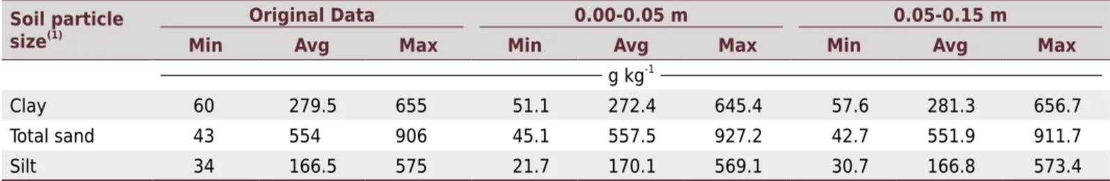
The statistical description of soil properties (sand, clay, and silt) based on soil sample analysis (original data and harmonized data) (0.00-0.05 and 0.05-0.15 m) is presented in table 2.
The Guapi-Macacu watershed exhibited substantial variability in soil types, predominantly Ferrasols - Latossolos (28 %), Acrisols - Argissolos (24 %), Cambisols - Cambissolos
(18 %), and Gleysols - Gleissolos (15 %). Soils with high sand content were common
along the Macacu and Guapi-Açu floodplains, which have wide texture variation due to river deposition systems and events. In the floodplains, particularly near river deltas and in estuarine deposits, Histic horizons and Gleysols with low pH (<4.5) were documented. Clayey soils show a wide area of distribution and were primarily derived from granite and gneiss parent materials. Some Acrisols have abrupt textural changes, with sandy surface horizons above clayey horizons (Santos et al., 2013). Parent materials of sedimentary rock origin are limited in the watershed and, in general, the soils formed have clayey textures and xanthic properties (WRB, 2014). A detailed analysis of soil-landscape relationships and soil genesis in the area can be consulted in Pinheiro et al. (2017).
The spline fitted curve of the profile (Figure 2) illustrates the original data (mean value corresponding to the depth of layer/horizon) and the harmonized data (fitted curve) according to the pre-defined depth intervals.
Table 2. Statistical description of soil properties based on soil samples of topsoil layer (original data and data harmonized to
0.00-0.05 and 0.00-0.05-0.15 m layers)
Soil particle
size(1)
Original Data 0.00-0.05 m 0.05-0.15 m
Min Avg Max Min Avg Max Min Avg Max
g kg-1
Clay 60 279.5 655 51.1 272.4 645.4 57.6 281.3 656.7
Total sand 43 554 906 45.1 557.5 927.2 42.7 551.9 911.7
Silt 34 166.5 575 21.7 170.1 569.1 30.7 166.8 573.4
The profile distribution of sand decreased with depth (Figure 2c). In contrast, the clay distribution increased substantially below 0.50 m of depth, and in the same layer, the silt fraction decreased drastically (Figures 2a and 2e). Silt content had decreasing values with depth to the bottom of the solum (approximately 1 meter). Below the solum depth, the increase in silt content in particular can be related the influence of weathered parental material. This textural pattern is typical for Haplic Ferralsols (Dystric), classified as Latossolo Vermelho-Amarelo according to the Brazilian System of Soil Classification - SiBCS (Santos et al., 2013), which are predominant in the watershed (Pinheiro et al., 2013). The spline function was executed on all sample point data to improve the capacity of preliminary results to predict the soil mineral fraction in the surface layer and to standardize the input database according to the GlobalSoilMap project (Arrouays et al., 2014).
Digital mapping of mineral soil particle size fraction
The linear models showed a greater range and more even distribution of output values compared to the predicted attributes. With the regression tree output, the values were discreet and points were often linear and parallel to the ‘x’ axis (Figures 3a, 3b, 3c, 3g, 3h, 3i, 3m, 3n, and 3o).
350
Original data and fitted spline Harmonized data
400 450 500 550
Depth (m)
0
1.00
2.00
350
Clay content (g kg-1)
400 450 500 550
350 400 450 500 550
0
1.00
2.00
350
Total sand content (g kg-1)
400 450 500 550
90 100 110 120
0
1.00
2.00
Silt content (g kg-1)
90 100 110 120
Figure 2. An example of clay, sand, and silt content variability with depth within a soil profile, with original data and harmonized
Original Data 0.00-0.05 m 0.05-0.15 m
R2
= 0.48 RMSE = 96.16
R2
= 0.52 RMSE = 99.48
R2
= 0.46 RMSE = 94.68
R2
= 0.42 RMSE = 101.35
R2
= 0.47 RMSE = 101.32
R2
= 0.40 RMSE = 106.35
R2
= 0.58 RMSE = 114.15
R2
= 0.56 RMSE = 120.68
R2
= 0.52 RMSE = 112.13
R2
= 0.38 RMSE = 138.43
R2
= 0.34 RMSE = 144.05
R2
= 0.39 RMSE = 139.61
R2
= 0.66 RMSE = 48.05
R2
= 0.65 RMSE = 48.95
R2
= 0.69 RMSE = 46.10
R2
= 0.51 RMSE = 57.68
R2
= 0.47 RMSE = 60.27
R2
= 0.51 RMSE = 57.66
Silt
content (g kg
-1)
Silt content (g kg-1)
RT
ML
R
Sand content (g kg
-1)
RT
ML
R
Clay content (g kg
-1)
Clay content (g kg-1)
Sand content (g kg-1)
RT ML R 150 200 250 300 350 400 150 200 250 300 350 400 450 150 200 250 300 350 400 450 100 200 300 400 500 100 200 300 400 500 100 200 300 400 500
100 200 300 400 500 600 100 200 300 400 500 600 100 200 300 400 500 600
300 400 500 600 700 800 300 400 500 600 700 800 300 400 500 600 700 300 400 600 700 800 150 200 250 300 350 150 200 250 300 350 100 200 250 300 350 100 150 200 250 350 100 200 250 300 350
200 400 600 800 200 400 600 800 200 400 600 800
500 300 400 600 700 800 500 300 400 600 700 800 500 200
100 200 300 400 500 100 200 300 400 500 100 200 300 400 500
150 50 100 100 200 250 300 350 50 100 300
(a) (b) (c)
(d) (e) (f)
(g) (h) (i)
(j) (k) (l)
(m) (n) (o)
(p) (q) (r)
Figure 3. Plotted results of clay, sand, and silt content predictions for the three input datasets (original data, and harmonized layers
In general, the RMSE showed low values when the original database was used, although the data range was large. The data range for sand was 112.13-144.05 g kg-1, for clay was 94.68-106.35 g kg-1, and for silt was 46.10-60.27 g kg-1. When utilizing the RT models, the output values according to the terminal nodes (leaves) and the plot results show a horizontal trend (Figure 3) that suggests a grouping of output values subordinated to the homogeneity of the output nodes. This homogeneity is intrinsic to the method since the output values are grouped in terminal nodes.
The RT models fitted the predicted results better than MLR models, and had the lowest values for RSME errors (94.68 for clay content, 112.13 for sand content, and 46.10 for silt content) suggesting better predicted results than the RLM models, which exhibited 101.32 for clay content, 138.43 for sand content, and 57.66 for silt content. These values were within the range that was proportional to the magnitude of the input data values. A lower RMSE is associated with greater predictive ability, but this index cannot be used to compare different properties since it depends directly on the scale of values (Henderson et al., 2005). Regarding clay content, the mean value for RSME was 103.00 for the MLR models and 96.78 for the RT models. The lowest index values were obtained for silt content, with a mean value of 46.10 for the RT models and 58.53 for the MLR models. The highest mean values of RSME were found in sand prediction (140.70 in MLR models and 115.65 in RT) due to the assumed natural range of sand content, which is larger than that of the other components. A detailed discussion about model performance is presented below.
Evaluation and selection of the models to represent topsoil texture
Results of predictive models (multiple linear regressions and regression trees) for the three soil properties and different input databases are summarized in table 3.
General analysis of the models primarily showed better performance of regression trees than multiple linear regressions for all three properties of mineral soil fraction content, regardless of the database used. Nussbaum et al. (2018) observed that linear regression models are unstable with a large number of covariates. The authors indicate that difficulties in working with datasets with a large number of covariates are chances of over-fitting calibration data, multi-collinearity, and noisy covariates. Unsatisfactory performance from linear regression models in predicting soil particle size, probably due to inter-correlation among covariates, was observed by Chagas et al. (2016).
Some positive aspects of the models were the ability to quickly tune parameters and to yield insight into decision rules and predictors. Vasques et al. (2008) had different results predicting total soil carbon, in which the stepwise multiple linear regressions showed better performance than regression tree models.
Sand content showed better performance in the regression tree models, in which all R2 values were greater than 0.52 in the RT models, and the highest value was 0.58.
Table 3. Summary of results for all models tested in the watershed according to soil particle size, model type, and depth
Soil property
Predictive model
Original data 0.00-0.05 m 0.05-0.15 m Variance(1)
R2
Adj R2
N R2
Adj R2
N R2
Adj R2
N R2
Adj R2
Clay MLR 0.42 0.32 15 0.47 0.16 15 0.40 0.30 15 0.0013 0.0076
RT 0.48 0.47 6 0.52 0.51 7 0.46 0.13 7 0.0009 0.0436
Sand MLR 0.38 0.28 13 0.34 0.25 12 0.39 0.29 13 0.0007 0.0004
RT 0.58 0.57 5 0.56 0.56 7 0.52 0.52 6 0.0009 0.0007
Silt MLR 0.51 0.39 19 0.47 0.36 17 0.51 0.40 18 0.0005 0.0004
RT 0.66 0.66 5 0.65 0.64 5 0.69 0.68 3 0.0004 0.0004
(1) Variance between coefficients of determination (R2 ); Adj R2
= adjusted R2
Meanwhile, multiple linear regressions had R2 values ranging from 0.34 to 0.39. Among the predicted soil properties, silt content had the best performance, in which all R2 values were higher than 0.65 in all RT models (Figure 3 and Table 3). Clay content prediction also showed better performance with RT models, reaching an R2 of 0.52 with the harmonized data in the 0.00-0.05 m layer; the lowest R2 value (0.46) was in the 0.05-0.15 m layer. The R² values in this study have higher correlations than the values described by Henderson et al. (2005) using tree-based models for prediction of particle size fractions in Australian topsoil layers (R2 values reaching 0.44). Similar values for mineral soil prediction were obtained by Sudduth et al. (2010) studying soils in Missouri (USA) where the clay, sand, and silt had R2 values of 0.56, 0.28, and 0.68, respectively. The values for clay and silt contents are considered relatively good, due to the high variability of these properties in soils. However, for sand content, the value are considered low. Lower values for soil texture prediction (average values of R2 lower than 0.20) were obtained by Carvalho Junior et al. (2014a) in a hillslope environment in Brazil, using the GlobalSoilMap harmonized depths.
The coefficient of determination (R2) is a well-known index used to evaluate regression
models. However, comparison between models with a different number of variables is more appropriate through the adjusted R2. This index is also useful in comparing models
with distinct input datasets, since the algorithm compensates for different sample sizes (Hair et al., 2009). The adjusted R2 and the R2 showed similar patterns of variability, with low values mostly ranging from 0.13 to 0.68 (Table 3). The variability of the predictive models for each soil property was compared through variance in the coefficients of determination, showing small values of variance between MLR and RT models; the greatest variability was related to clay prediction. Carvalho Junior et al. (2004a) observed similar performance between MLR and RT models used to predict soil texture components.
Concerning the number of covariates, the best performance model (R2 = 0.69) used the lowest number of terrain variables (3), which suggests a strong correlation among those terrain variables (band 4 of Landsat, the clay mineral index, and the protection index) and the silt content. In general, the RT models used 3 to 7 covariates, and an average of 6 covariates.
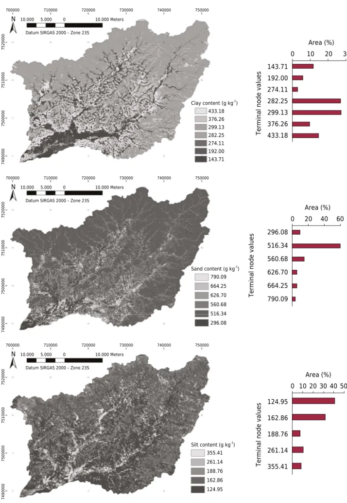
Tree models produced discreet output values in the terminal nodes (leaves), and for that reason, they were considered a good technique for separating a dataset into homogeneous groups. The range of terminal nodes was from 5 to 8, with an average of 7. Similar results regarding the number of covariates and terminal nodes of regression trees was demonstrated by Vasques et al. (2008) for soil carbon prediction when models used, on average, seven covariates and ten terminal nodes. Figure 4 presents the maps of the soil mineral fractions with the terminal node values related to the area.
In general, the surface horizons of soils in the watershed showed sand contents higher than silt and clay, as observed in the field survey. This was correlated with the soil classes, predominantly Ferrasols and Acrisols, with a clay content increasing along with soil depth. Another reason is the occurrence of surface laminar erosion and landslides, removing finer soil particles, such as silt and clay, due to steep slopes that are common in the watershed, as observed by Pinheiro et al. (2017). This may be observed in figure 4, particularly in the northern portion of the watershed within the mountain range, which showed high values of sand content. These observations were corroborated in the field survey and by interpretation of analytical data.
Area (%)
0 10 20 30
Area (%)
0 20 40 60
Area (%)
0 1020 30 40 50
Terminal node values
143.71
192.00
282.25
376.26 274.11
299.13
433.18
Terminal node values
296.08
560.68
664.25 516.34
626.70
790.09
Terminal node values
124.95
162.86
261.14 188.76
355.41
Silt content (g kg-1)
355.41
261.14
188.76
162.86
124.95
Sand content (g kg-1
)
790.09
664.25
626.70
560.68
516.34
296.08
Clay content (g kg-1)
433.18
376.26 299.13
282.25 274.11
192.00 143.71
N
Datum SIRGAS 2000 – Zone 23S
10.000 5.000 0 10.000 Meters
700000 710000 720000 730000 740000 750000
7490000
7500000
7510000
7520000
N
Datum SIRGAS 2000 – Zone 23S
10.000 5.000 0 10.000 Meters
700000 710000 720000 730000 740000 750000
7490000
7500000
7510000
7520000
N
Datum SIRGAS 2000 – Zone 23S
10.000 5.000 0 10.000 Meters
700000 710000 720000 730000 740000 750000
7490000
7500000
7510000
7520000
Figure 4. Prediction maps for sand (original data), clay (0.00-0.05 m), and silt (0.05-0.15 m) contents in the watershed with the
(Figure 4), more than 54 % of the watershed area had clay content in the topsoil layer, ranging from 280 to 300 g kg-1. In contrast, greater sand contents were related to active
floodplains and the sand content was lowest at the mouth of the watershed where clay content was highest due to the depositional environment. In this area, the topsoil has the highest values of total organic carbon, which is also related to the estuarine depositional environment near sea level.
In general, the soils in the watershed had irregular distribution of silt, with a trend of high silt content where Fluvisols predominate. Areas with high silt content in the surface layer were also identified in landscapes with a steep slope in the mountain range, with poorly developed soils (Regosols) and the presence of rock outcrops. Both types of soils show the strong influence of parental material enhancing an incipient pedogenic process and structural development.
The main differences in the final products (attribute maps) are inherent to the models since the RT model produces discreet output values corresponding to each terminal node (Vasques et al., 2008), instead of the wide range of continuous values presented by the MLR models.
The analysis indicated that differences among databases (original and harmonized data) were small, which suggests that they can likewise be used for modeling. Thus, soil scientists are encouraged to harmonize their data, as proposed by the GlobalSoilMap project, and in this way contribute to the global soil database of soil properties.
The products from the digital mapping approach may enhance soil survey reports, providing easier interpretation for soil management and the uncertainties associated with soil property predictions. Additionally, the digital soil map products provide higher resolution property predictions, which can be combined to develop many use-oriented indexes to target particular management issues related to soil-landscape function. All these beneficial outcomes from digital soil mapping can be used to address land use decisions in the Guapi-Macacu watershed, Rio de Janeiro, and other locations where these maps are developed.
CONCLUSIONS
The regression tree models performed better for all the predicted properties and soil depths tested, although multiple linear regression showed similar results. The harmonized dataset at the 0.00-0.05 and 0.05-0.15 m layers, in general, had better results for clay and silt properties, with values of 0.52 for clay in the 0.00-0.05 m layer, and 0.69 for silt in the 0.05-0.15 m layer. The prediction of sand content showed better results with the original data depth as input, although all regression tree models for this attribute had R2 values greater than 0.52, and small variance
among them (0.0007). Variance between the coefficients of determination was small; thus, both databases (original and harmonized) may equally be applied to modeling the soil properties in the watershed.
The generalization of soil texture components (sand, clay, and silt) performed by the regression tree methods were consistent with field observations and the watershed landscape characteristics. This evidence supports a relationship between terrain attributes and topsoil properties, which can be determined by field observations and model predictions.
ACKNOWLEDGMENTS
Our thanks to the Federal Rural University of Rio de Janeiro - Agronomy Institute (Brazil), Embrapa Solos (Brazil), Purdue University - Department of Agronomy (United States), and the Coordination of Improvement of Higher Level Personnel - Capes (Brazil), which supported this study by providing the expertise of professors/researchers, infrastructure, software licenses, and funding.
REFERENCES
Arrouays D, McKenzie N, Hempel J, Forges AR, McBratney A. GlobalSoilMap: basis of the global spatial soil information system. Netherlands: CRC Press/Balkema; 2014.
Arrouays D, Vion I, Kicin JL. Spatial analysis and modeling of topsoil carbon storage in temperate forest humic loamy soils of France. Soil Sci. 1995;159:191-8.
https://doi.org/10.1097/00010694-199503000-00006
Berry WD, Feldman S. Multiple regression in practice: quantitative applications in the social sciences. Beverly Hills: Sage Publications, Inc.; 1985. (Sage University Paper - Book 50).
Beven K, Binley A. The future of distributed models: model calibration and uncertainty prediction. Hydrol Process. 1992;6:279-98. https://doi.org/10.1002/hyp.3360060305
Bishop TFA, McBratney AB, Laslett GM. Modelling soil attribute depth functions with equal-area quadratic smoothing splines. Geoderma. 1999;91:27-45.
https://doi.org/10.1016/S0016-7061(99)00003-8
Böhner J, Antonic O. Land-surface parameters specific to topo-climatology. Dev Soil Sci. 2009;33:195-226. https://doi.org/10.1016/S0166-2481(08)00008-1
Böhner J, Conrad O. Module relative heights and slope positions. SAGA - System for automated geoscientific analyses; 2007. Available at: www.saga-gis.org/saga_tool_doc/2.2.6/ta_
morphometry_14.html
Böhner J, Köthe R, Conrad O, Gross J, Ringeler A, Selige T. Soil regionalisation by means of terrain analysis and process parameterisation. In: Micheli E, Nachtergaele FO, Jones RJA, Montanarella L, editors. Soil Classification 2001. Luxembourg: European Communities; 2002. p. 213-22. (European Soil Bureau Research Report No. 7).
Böhner J, Selige T. Spatial prediction of soil attributes using terrain analysis and climate
regionalisation. In: Böhner J, McCloy KR, Strobl J. SAGA - Analysis and modelling applications. v. 115. Göttingen: Verlag Erich Goltze GmbH; 2006. p. 13-27. (Göttinger Geographische Abhandlungen). Breiman L, Friedman J, Olshen R, Stone C. Classification and regression trees: the Wadsworth statistics/probability series. Belmont: Wadsworth International; 1984.
Brenning A. Benchmarking classifiers to optimally integrate terrain analysis and multispectral remote sensing in automatic rock glacier detection. Remote Sens Environ. 2009;113:239-47. https://doi.org/10.1016/j.rse.2008.09.005
Brůna J, Wild J, Svoboda M, Heurich M, Müllerovà J. Impacts and underlying factors of landscape-scale, historical disturbance of mountain forest identified using archival documents. Forest Ecol Manag. 2013;305:294-306. https://doi.org/10.1016/j.foreco.2013.06.017
Carvalho Junior W, Lagacherie P, Chagas CS, Calderano Filho B, Bhering SB. A regional-scale assessment of digital mapping of soil attributes in a tropical hillslope environment. Geoderma. 2014a;232-234:479-86. https://doi.org/10.1016/j.geoderma.2014.06.007
Carvalho Junior W, Chagas CS, Muselli A, Pinheiro HSK, Pereira NR, Bhering SB. Método do hipercubo latino condicionado para a amostragem de solos na presença de covariáveis ambientais visando o mapeamento digital de solos. Rev Bras Cienc Solo. 2014b;38:386-96. https://doi.org/10.1590/S0100-06832014000200003
Chagas CS, Vieira CAO, Fernandes Filho EI. Comparison between artificial neural networks and maximum likelihood classification in digital soil mapping. Rev Bras Cienc Solo. 2013;37:339-51. https://doi.org/10.1590/S0100-06832013000200005
Claessen MEC, organizador. Manual de métodos de análise de solo. 2. ed. Rio de Janeiro: Embrapa Solos; 1997.
Costa‐Cabral MC, Burges SJ. Digital elevation model networks (DEMON): a model of flow over hillslopes for computation of contributing and dispersal areas. Water Resour Res. 1994;30:1681-92. https://doi.org/10.1029/93WR03512
Cunha AM. Seleção de variáveis ambientais e de algoritmos de classificação para mapeamento digital de solos [tese]. Viçosa, MG: Universidade Federal de Viçosa; 2013.
Deng Y, Wilson JP, Gallant JC. Terrain analysis. In: Wilson JP, Fotheringham AS. The handbook of geographic information science. Malden: Blackwell Publishing; 2008. p. 417-35.
https://doi.org/10.1002/9780470690819.fmatter
Dobos E, Micheli E, Baumgardner MF, Biehl L, Helt T. Use of combined digital elevation model and satellite radiometric data for regional soil mapping. Geoderma. 2000;97:367-91.
https://doi.org/10.1016/S0016-7061(00)00046-X
Donagema GK, Campos DVB, Calderano SB, Teixeira WG, Viana JHM, organizadores. Manual de métodos de análise do solo. 2. ed rev. Rio de Janeiro: Embrapa Solos; 2011.
Eldeiry AA, Garcia LA. Detecting soil salinity in alfalfa fields using spatial modeling and remote sensing. Soil Sci Soc Am J. 2008;72:201-11. https://doi.org/10.2136/sssaj2007.0013
Environmental Systems Research Institute - Esri. ArcGIS and ArcINFO [computer program]. Version 10.0. Redlands: 2010.
Erdas Systems. Erdas Imagine. Version 9.1. Maryland: 2008.
Faraway JJ. Practical Regression and Anova Using R. United Kingdom: University of Bath; 2000.
Fernandez-Illescas CP, Porporato A, Laio F, Rodriguez-Iturbe I. The ecohydrological role of soil texture in a water-limited ecosystem. Water Resour Res. 2001;37:2863-72.
https://doi.org/10.1029/2000WR000121
Ferrari AL. Evolução tectônica do Gráben da Guanabara [tese]. São Paulo: Universidade de São Paulo; 2001.
Fidalgo ECC, Pedreira BCCG, Abreu MB, Moura IB, Godoy MDP. Uso e cobertura da terra na bacia hidrográfica do rio Guapi-Macacu. Rio de Janeiro: Embrapa Solos; 2008. (Documentos 105). Figueiredo SR. Mapeamento supervisionado de solos através do uso de regressões logísticas múltiplas e sistema de informações geográficas [dissertação]. Porto Alegre: Universidade Federal do Rio Grande do Sul; 2006.
Florinsky IV, Eilers RG, Manning GR, Fuller LG. Prediction of soil properties by digital terrain modeling. Environ Modell Softw. 2002;17:295-311. https://doi.org/10.1016/S1364-8152(01)00067-6 Freeman GT. Calculating catchment area with divergent flow based on a regular grid. Comp Geosc. 1991;17:413-22. https://doi.org/10.1016/0098-3004(91)90048-I
Gallant JC, Dowling TI. A multiresolution index of valley bottom flatness for mapping
depositional areas. Water Resour Res. 2003;39:1347. https://doi.org/10.1029/2002WR001426
Geographic Resources Analysis Support System - GRASS. Software: GRASS is Copyright, 1999-2013. Available at: http://grass.osgeo.org/home/copyright/. 2013.
Gessler PE, Moore ID, McKenzie NJ, Ryan PJ. Soil-landscape modelling and spatial prediction of soil attributes. Int J Geogr Inf Syst. 1995;9:421-32. https://doi.org/10.1080/02693799508902047
Gökceoglu C, Aksoy H. Landslide susceptibility mapping of the slopes in the residual soils of the Mengen region (Turkey) by deterministic stability analyses and image processing techniques. Eng Geol. 1996;44:147-61. https://doi.org/10.1016/S0013-7952(97)81260-4
Gozdowski D, Stępień M, Samborski S, Dobers ES, Szatyłowicz J, Chormański J. Determination of the most relevant soil properties for the delineation of management zones in production fields. Commun Soil Sci Plan. 2014;45:2289-304. https://doi.org/10.1080/00103624.2014.912289
Grimaldi S, Nardi F, Di Benedetto F, Istanbulluoglu E, Bras RL. A physically-based method for removing pits in digital elevation models. Adv Water Resour. 2007;30:2151-8.
https://doi.org/10.1016/j.advwatres.2006.11.016
Hair JF, Black WC, Babin BJ, Anderson RE, Tatham RL. Análise multivariada de dados. 6. ed. Porto Alegre: Bookman; 2009.
Hall GF, Olson CG. Predicting variability of soils from landscape models. In: Mausbach MJ, Wilding LP, editors. Spatial variabilities of soils and landforms. Madison: Soil Science Society of America; 1991. p. 9-24. https://doi.org/10.2136/sssaspecpub28.c2
Häring T, Dietz E, Osenstetter S, Koschitzki T, Schröder B. Spatial disaggregation of complex soil map units: a decision-tree based approach in Bavarian forest soils. Geoderma.
2012;185-186:37-47. https://doi.org/10.1016/j.geoderma.2012.04.001
He Y, Wei Y, DePauw R, Qian B, Lemke R, Singh A, Cuthbert R, McConkey B, Wang H. Spring wheat yield in the semiarid Canadian prairies: effects of precipitation timing and soil texture over recent 30 years. Field Crop Res. 2013;149:329-37. https://doi.org/10.1016/j.fcr.2013.05.013
Henderson BL, Bui EN, Moran CJ, Simon DAP. Australia-wide predictions of soil properties using decision trees. Geoderma. 2005;124:383-98. https://doi.org/10.1016/j.geoderma.2004.06.007
Hengl T. A practical guide to geostatistical mapping. 2nd ed. Amsterdam: University of Amsterdam; 2009.
Hora AF, Hwa CS, Hora MAGM. Projeto Macacu: planejamento estratégico da região hidrográfica dos rios Guapi-Macacu e Caceribu-Macacu. Niterói: Universidade Federal Fluminense/Fundação Euclides da Cunha; 2010.
Hutchinson MF, Gallant JC. Digital elevation models and representation of terrain shape. In: Wilson JP, Gallant JC, editors. Terrain analysis: principles and applications. New York: John Wiley & Sons; 2000. p. 29-50.
Jasiewicz J, Stepinski TF. Geomorphons - a pattern recognition approach to classification and mapping of landforms. Geomorphology. 2013;182:147-56.
https://doi.org/10.1016/j.geomorph.2012.11.005
Jenny H. The soil resource: origin and behaviour. New York: Springer-Verlag; 1980. (Ecological Studies, 37).
Klingebiel AA. Land classification for use in planning. Washington, DC: Yearbook of Agriculture; 1963.
Lea NJ. An aspect-driven kinematic routing algorithm. In: Parsons AJ, Abrahams AD, editors. Overland flow: hydraulics and erosion mechanics. London: Routledge; 1992. p. 374-88. Leão MGA, Marques Júnior J, Souza ZM, Pereira GT. Variabilidade espacial da textura de um Latossolo sob cultivo de citros. Cienc Agrotec. 2010;34:121-31.
https://doi.org/10.1590/S1413-70542010000100016
Leão MGA, Marques Júnior J, Souza ZM, Siqueira DS, Pereira GT. Terrain forms and spatial variability of soil properties in an area cultivated with citrus. Eng Agric. 2011;31:643-51. https://doi.org/10.1590/S0100-69162011000400003
Ließ M, Glaser B, Huwe B. Uncertainty in the spatial prediction of soil texture: comparison of regression tree and Random Forest models. Geoderma. 2012;170:70-9.
https://doi.org/10.1016/j.geoderma.2011.10.010
Ließ M, Hitziger M, Huwe B. The sloping mire soil-landscape of Southern Ecuador: influence of predictor resolution and model tuning on random forest predictions. Appl Environ Soil Sci. 2014;3014:1-10. https://doi.org/10.1155/2014/603132
Marques Júnior J, Lepsch IF. Depósitos superficiais neocenozóico, superfícies geomórficas e solos em Monte Alto, SP. Geociências. 2000;19:265-81.
McBratney AB, Odeh IOA, Bishop TFA, Dunbar MS, Shatar TM. An overview of pedometric techniques for use in soil survey. Geoderma. 2000;97:293-327.
https://doi.org/10.1016/S0016-7061(00)00043-4
Mcbratney AB, Santos MLM, Minasny B. On digital soil mapping. Geoderma. 2003;117:3-52. https://doi.org/10.1016/S0016-7061(03)00223-4
Minasny B, McBratney AB. A conditioned Latin hypercube method for sampling in the presence of ancillary information. Comput Geosci. 2006;32:1378-88.
https://doi.org/10.1016/j.cageo.2005.12.009
Minasny B, McBratney AB, Malone BP, Wheeler I. Digital mapping of soil carbon. Adv Agron. 2013;118:1-47. https://doi.org/10.1016/B978-0-12-405942-9.00001-3
Minasny B, McBratney AB, Mendonça-Santos ML, Santos HG. Revisão sobre funções de pedotransferência (PTFs) e novos métodos de predição de classes e atributos do solo. Rio de Janeiro: Embrapa Solos; 2003. (Documentos 45).
Möller M, Volk M. Effective map scales for soil transport process and related process domains – statistical and spatial characterization of their scale-specific inaccuracies. Geoderma.
2015;247-248:151-60. https://doi.org/10.1016/j.geoderma.2015.02.003
Möller M, Volk M, Friedrich K, Lymburner L. Placing soil‐genesis and transport processes into a landscape context: a multiscale terrain‐analysis approach. J Plant Nutr Soil Sci.
2008;171:419-30. https://doi.org/10.1002/jpln.200625039
Moore ID, Gessler PE, Nielsen GA, Peterson GA. Soil attribute prediction using terrain analysis. Soil Sci Soc Am J. 1993;57:443-52. https://doi.org/10.2136/sssaj1993.03615995005700020026x
Moore ID, Grayson RB, Ladson AR. Digital terrain modelling: a review of hydrological. geomorphological and biological applications. Hydrology Processes. 1991;5:3-30. https://doi.org/10.1002/hyp.3360050103
Moriasi DN, Arnold JG, Van Liew MW, Bingner RL, Harmel RD, Veith TL. Model evaluation guidelines for systematic quantification of accuracy in watershed simulations. ASABE. 2007;50:885-900. https://doi.org/10.13031/2013.23153
Nguyen MQ, Atkinson PM, Lewis HG. Superresolution mapping using a hopfield neural network with fused images. IEEE T Geosci Remote. 2006;44:736-49.
https://doi.org/10.1109/TGRS.2005.861752
Nussbaum M, Spiess K, Baltensweiler A, Grob U, Keller A, Greiner L, Schaepman ME, Papritz A. Evaluation of digital soil mapping approaches with large sets of environmental covariates. Soil Discuss. 2018;4:1-22. https://doi.org/10.5194/soil-2017-14
Odeh IOA, McBratney AB, Chittleborough DJ. Spatial prediction of soil properties from landform attributes derived from a digital elevation model. Geoderma. 1994;63:197-214.
https://doi.org/10.1016/0016-7061(94)90063-9
Odgers NP, Libohova Z, Thompson JA. Equal-area spline functions applied to a legacy soil database to create weighted-means maps of soil organic carbon at a continental scale. Geoderma. 2012;189-190:153-63. https://doi.org/10.1016/j.geoderma.2012.05.026
Olaya V. A gentle introduction to SAGA GIS. Germany: The SAGA user group eV; 2004.
Pinheiro HSK, Anjos LHC, Chagas CS. Mapeamento digital de solos por redes neurais artificiais - estudo de caso: bacia hidrográfica do rio Guapi-Macacu, RJ. Germany: Novas Edições Acadêmicas; 2013.
Pinheiro HSK, Chagas CS, Carvalho Júnior W, Anjos LHC. Modelos de elevação para obtenção de atributos topográficos utilizados em mapeamento digital de solos. Pesq Agropec Bras.
2012;47:1384-94. https//doi.org/10.1590/S0100-204X2012000900024
Ponce-Hernandez R, Marriott FHC, Beckett PHT. An improved method for reconstructing a soil profile from analyses of a small number of samples. J Soil Sci. 1986;37:455-67.
https://doi.org/10.1111/j.1365-2389.1986.tb00377.x
Prates V, Souza LCP, Oliveira Junior JC. Índices para a representação da paisagem como apoio para levantamento pedológico em ambiente de geoprocessamento. R Bras Eng Agric Ambient. 2012;16:408-14. https://doi.org/10.1590/S1415-43662012000400011
Quinn P, Beven K, Chevallier P, Planchon O. The prediction of hillslope flow paths for distributed hydrological modelling using digital terrain models. Hydrol Process. 1991;5:59-79.
https://doi.org/10.1002/hyp.3360050106
R Development Core Team. R: A language and environment for statistical computing. R Foundation for Statistical Computing, Vienna, Austria; 2014 [accessed on 09 Jun 2014]. Available at: http://www.R-project.org/.
Resende M, Curi N, Santana DP. Pedologia e fertilidade do solo: Interações e aplicações. Brasília: Ministério da Educação; 1988.
Roudier P, Hewitt AE, Beaudette DE. A conditioned Latin hypercube sampling algorithm incorporating operational constraints. In: Minasny B, Malone BP, McBratney AB. Digital soil assessments and beyond: proceedings of the 5th Global workshop on digital soil mapping. Sydney: CRC Press; 2012. p. 227-32.
Sabins FF. Remote sensing for mineral exploration. Ore Geol Rev. 1999;14:157-83. https://doi.org/10.1016/S0169-1368(99)00007-4
Sabins FF. Remote sensing: principles and interpretation. 3rd ed. New York: Waveland Press, Inc.; 1997.
Sandmeier S, Itten KI. A physically-based model to correct atmospheric and illumination effects in optical satellite data of rugged terrain. IEEE T Geosci Remote. 1997;35:708-17.
https://doi.org/10.1109/36.581991
Santos HG, Jacomine PKT, Anjos LHC, Oliveira VA, Oliveira JB, Coelho MR, Lumbreras JF, Cunha TJF. Sistema brasileiro de classificação de solos. 3. ed. rev. ampl. Rio de Janeiro: Embrapa Solos; 2013.
Silver WL, Neff J, McGroddy M, Veldkamp E, Keller M, Cosme R. Effects of soil texture on belowground carbon and nutrient storage in a lowland Amazonian forest ecosystem. Ecosystems. 2000;3:193-209. https://doi.org/10.1007/s100210000019
Sudduth KA, Kitchen NR, Sadler EJ, Drummond ST, Myers DB. VNIR spectroscopy estimates of within-field variability in soil properties. In: Rossel RAV, McBratney AB, Minasny B, editors. Proximal soil sensing. New York: Springer; 2010. p. 153-64.
System for Automated Geoscientific Analyses - SAGA. Software: SAGA Version: 2.1.4. SAGA-GIS. org; 2007. Available at: http://www.saga-gis.org.
System for Automated Geoscientific Analyses - SAGA. Module valley depth. System for Automated Geoscientific Analyses. SAGA-GIS.org; 2012. Available at: http: www.saga-gis.org/ saga_tool_doc/2.2.6/ta_morphometry_14.html
Tarini M, Cignoni P, Montani C. Ambient occlusion and edge cueing to enhance real time molecular visualization. IEEE T Geosci Remote. 2006;12:1237-44.
https://doi.org/10.1109/TVCG.2006.115
Therneau T, Atkinson B, Ripley B. Package ‘rpart’: recursive partitioning and regression trees. Version 4.1-11. R package; 2017. Available at: ftp://cran.r-project.org/pub/R/web/packages/ rpart/rpart.pdf.
Thompson JA, Bell JC, Butler CA. Digital elevation model resolution: effects on terrain attribute calculation and quantitative soil-landscape modeling. Geoderma. 2001;100:67-89.
https://doi.org/10.1016/S0016-7061(00)00081-1
Vasques GM, Grunwald S, Sickman JO. Comparison of multivariate methods for inferential modeling of soil carbon using visible/near-infrared spectra. Geoderma. 2008;146:14-25. https://doi.org/10.1016/j.geoderma.2008.04.007
White RE. Principles and practice of soil science: the soil as a natural resource. 4th ed. Oxford: Blackwell; 2006.
Wilson JP, Gallant JC. Terrain analysis: principles and applications. New York: John Wiley & Sons, Inc; 2000.
Word Reference Base for Soil Resources - WRB: International soil classification system for naming soils and creating legends for soil maps. Food and Agriculture Organization of the United Nations. Rome: IUSS/ISRIC/FAO; 2014. (World Soil Resources Reports, 106).
Yang W, Yang L, Merchant JW. An assessment of AVHRR/NDVI-ecoclimatological relations in Nebraska, U.S.A. Int J Remote Sens. 1997;18:2161-80. https://doi.org/10.1080/014311697217819
Yokoyama R, Shirasawa M, Pike RJ. Visualizing topography by openness: a new application of image processing to digital elevation models. Photogramm Eng Rem S. 2002;68:257-65.
Young P, Parkinson S, Lees M. Simplicity out of complexity in environmental modelling: Occam’s razor revisited. J Appl Stat. 1996;23:165-210. https://doi.org/10.1080/02664769624206
Zakšek K, Oštir K, Kokalj Ž. Sky-view factor as a relief visualization technique. Remote Sens. 2011;3:398-415. https://doi.org/10.3390/rs3020398