PREDICTING KAPPA NUMBER IN A KRAFT PULP CONTINUOUS DIGESTER: A COMPARISON OF FORECASTING METHODS

of Chemical

Engineering

ISSN 0104-6632 Printed in Brazil www.scielo.br/bjce Vol. 35, No. 03, pp. 1081-1094, July - September, 2018

dx.doi.org/10.1590/0104-6632.20180353s20160678

PREDICTING KAPPA NUMBER IN A KRAFT PULP

CONTINUOUS DIGESTER: A COMPARISON OF

FORECASTING METHODS

Flávio Marcelo Correia

_{*, José Vicente Hallak d’Angelo}

_,

Gustavo Matheus Almeida

_{and Sueli Aparecida Mingoti}

1 _{CENIBRA Celulose Nipo Brasileira SA}

2 _{UNICAMP – University of Campinas, School of Chemical Engineering} 3 _{UFMG – Federal University of Minas Gerais, Dep. of Chemical Engineering}

4 _{UFMG – Federal University of Minas Gerais, Dep. of Statistics}

(Submitted: December 16, 2016; Revised: August 24, 2017; Accepted: October 23, 2017)

Abstract - This paper discusses kappa number prediction models using Single Exponential Smoothing, Multiple Linear Regression Analysis, the Time Series Method of Box-Jenkins (ARIMA) and Artificial Neural Networks. Applying a database of an industrial eucalyptus Kraft pulp continuous digester, these four different methods were evaluated according to different statistical decision criteria. After fitting the parameters of the models, validations were performed using a new dataset. Results, advantages and limitations of the four methods were compared. Some statistical forecasting indexes indicate that the ARIMA model showed more accurate estimation results, achieving a MAPE lower than 3 % and over 90% of the prediction data deviations lower than one kappa unit.

Keywords: Kraft pulping; Continuous digester; Statistical methods; Neural network applications.

INTRODUCTION

Complex processes with significant time delays are difficult to optimize and control. An example of

such a process in the Kraft pulp mill is continuous cooking, which is the dominant pulping method in modern mills (Pikka and Andrade, 2015). The role of the pulp digester is to remove lignin from wood chips. Kappa number is the most used index for measuring residual lignin present in the pulp (Costa and Colodette, 2007). It is measured either using online concentration analyzers, or in the laboratory by lignin oxidation with potassium permanganate under acidic conditions. The digester primary control objective is to produce uniform pulp with minimum

variability, contributing to keep quality and stability

in the following fiber line steps. A low kappa number affects negatively pulp strengths because of the

carbohydrate dissolution, resulting in a substantial loss in pulp yield. On the other hand, the main production failure in a continuous digester occurs when a high kappa number pulp is achieved, which raises the bleaching chemicals costs, organic charge

to the effluent treatment station and plugging risks

at the screen plant as well (which forces reduction of the production). In recent years, regarding pulp yield aspects, the trend in bleachable-grade chemical pulping has been to push the kappa number as high as

possible, just below the fiber liberation point (Weding,

2012; Hart, 2014). Thereby, considering the natural

wood quality variations, long residence time and the tendency of the mills to end the cooking at a higher kappa number, a better accuracy in kappa number control is a keynote to digester operation.

Making a forecast is to predict a future observation. Forecasting is an important issue for manufacturing companies. Several decision making processes need accurate forecasts in order to choose proper actions

relevant to different production aspects. For this

reason, over the years practitioners and academics have devoted particular attention to how forecasting can be improved to increase forecast accuracy (Danese and Kalchschmidt, 2011).

Artificial Neural Networks and statistical methods are widely reported for different chemical engineering

applications (Assidjo et al., 2008; Kazemi-Beydokhti et al., 2015). Kappa number prediction models are useful in cases where an on-line analyzer is not available, or as an inferential sensor to be used as an additional kappa number indicator, giving a warning to the operators when large discrepancies are observed (between measured and estimated values), as a reference model for device calibration monitoring or for a better understanding of the process behavior as

well. With a kappa number inference, more information

can be achieved and then used to determine actions to control the process in advance.

In this context, the objective of this study is to

compare performance of different dynamic inferential

models for kappa number prediction. Four methods - Single Exponential Smoothing (SES), Box-Jenkins (ARIMA), Multiple Linear Regression Analysis

(MLR) and Artificial Neural Networks (ANN) were

used to formulate and compare the kappa number inferential capability of a eucalyptus Kraft pulp continuous digester. Advantages and limitations of these four methods were discussed.

Kraft Pulping Continuous Digester

The kraft pulp continuous digester is a tubular reactor where wood chips react with an aqueous

solution of sodium hydroxide and sodium sulfide

(referred to as white liquor) to remove lignin from

cellulose fibers. Most continuous digesters consist of

three basic zones: impregnation, cooking and washing,

where the flow of white liquor is either co-current or counter-current with respect to the chips flow (Smook,

1992).

White liquor penetrates and diffuses into the wood chips as it flows down through the impregnation zone.

The mix is heated to a target cooking temperature

where bulk delignification starts, and the majority of

lignin is removed. The cooking process is stopped at the beginning of the washing zone by reducing the temperature and then cooked pulp is washed in a counter-current washing zone, using wash liquor injected at the bottom of the digester.

Various factors affect the overall Kraft pulping reaction rate, including thermal and fluid dynamic factors, liquor and chip diffusion characteristics and the delignification reactions (Gullichsen, 2000; MacLeod,

2007). Continuous Kraft pulping is a complex process by its nature. Some of the reasons are raw material variability, long time delays involved, non-linear behavior, complexity of chip column dynamics, operational disturbances, scarce availability of process measurements and strong interdependencies between process stages and variables (Kocurek et al., 1989; Lindstrom, 2007). Continuous cooking is one of the major unit operations in the pulp mill and its proper control determines the quality characteristics of the brown stock pulp and subsequent stages.

Kraft Pulping Modeling

Regardless of whether new or existing processes are to be modelled, the objectives of the data analyses may be used in monitoring the state of the process. Understanding the relationship between factors and responses, process diagnosis and optimization allows operators to follow the process behavior when it shifts from one condition to another. In this context, anticipating demand changes is critical in the process industry with high capacity utilization (Blackburn et al., 2015).

Models may be divided into theoretical and empirical ones. Theoretical models explain the nature

of the reactions, phenomena and different process

conditions. Empirical models are based on experimental data. Kraft pulping has been modeled to various levels of complexity. The development of chemical reaction rate expressions that take place during Kraft pulping is arduous because of the heterogeneous nature of the system, multivariable and interactive chemical and physical processes and long residence times. Nonetheless, modeling and simulation of pulping processes have become valuable tools to the pulp and paper industries (Dahlquist, 2008).

process predictive model control tools (Badwe, 2016; Rahman et al., 2017).

In contrast, some researchers have used software computing methods developing empirical predictive

models for kappa number using different data-driven

approaches. An ANN-based strategy for detection of feedstock variations in a continuous pulp digester were studied by Dufour et al. (2005). Wood chip

moisture content and densities and alkali and sulfidity

in the white liquor were modeled in a pilot plant. Ahvenlampi and Kortela (2005) developed a kappa number prediction model and fault diagnostics of continuous digesters using clustering techniques.The results showed the usability of the combined hybrid system in the monitoring of the process and the kappa number prediction. Halmevaara (2009) developed a novel method using multivariate regression to capture the dependencies among the system parameters and quality measures for large industries, presenting results of regression adjustments as an interactive case study simulation of a double vessel softwood pulp continuous digester. Araneda et al. (2009) adapted the Purdue model to the physical characteristics of a Kamyr digester. This model was able to represent satisfactorily both dynamic and steady states of the digester operation, improving information from previous models. Predicted data obtained from this model were compared to measured ones from mills, such as blow-line kappa number, yield, free

liquor temperature profile, and pulp production rate.

Saavedra (2011) selected 29 cooking variables from his experience with a continuous digester, and used a MLR and ANN for predictive models, concluding that the ANN presented better results. Galicia et. al (2012) applied soft sensors using secondary measurements based on multivariate regression techniques. They developed a software sensor in order to reduce the number of regressor variables and also to provide superior prediction performance of kappa number applied in both simulated and industrial continuous Kamyr digester case studies. Kraft pulping has been a widely studied subject, especially concerning softwood pulp. Nevertheless, there are only a few references to kappa number prediction techniques concerning

statistical and artificial neural network models from

industrial hardwood pulping data. In this sense, this work brings an important contribution to the studies involving hardwood processing.

METHODS

Time series analysis and forecasting has become

a valuable tool in different applications. The ability

to forecast optimally, understanding the dynamic relationships between variables, is of great practical importance (Hair et al. 2009). If physical interpretation is less important and a complex system needs to be described by a simple input-output model, a data driven approach may be applied. This observed behavior is mapped by a mathematical representation that does not have a physical basis. Much statistical methodology is concerned with models in which the observations are assumed to vary independently. In many applications the dependence between the observations is regarded as a challenge, and in planned experiments, randomization of the experimental design is introduced to validate analysis conducted as if the observations were independent. However, many data in engineering and industries occur in the form of time series (a set of observation generated sequentially in time), where observations are dependent and where the nature of this dependence itself is of interest (Chase Jr., 2013). The body of techniques available for the analysis of such series of dependent observations is

called time series analysis, which may be classified as

linear or nonlinear. In this paper two univariate (SES and ARIMA) and two multivariate methods (MLR and

ANN) are evaluated and they are briefly described as

follows.

Single Exponential Smoothing (SES)

Single Exponential Smoothing is a method used

to smooth and forecast a time series without fitting

parameters of a model. It is based on a recursive computing scheme, where the forecasts are updated for each new incoming observation. Exponential smoothing is considered a simple prediction technique, yet it is used in practice where it shows good performance (Makridakis et al., 1983). It is used for short-range forecasting, usually just one step into the future. The model requires a large number of

observations, assumes that the data fluctuate around a

reasonably stable mean, i.e., it is not appropriate for data that has a seasonal component, trend or consistent pattern of growth (Holt, 2004). The formula for simple exponential smoothing is expressed as:

(1)

When applied recursively to each successive

observation in the series, each new smoothed value (forecasted Ŷ_t) is computed as the weighted average

(given by α) of the current observation (Y_t-1) and the previous smoothed observation (Y_t-1). The previous smoothed observation was computed in turn from

(

)

the previous observed value and the smoothed value before the previous observation, and so on.

Multiple Linear Regression (MLR)

Multiple Regression analysis is one of the most popular statistical estimation procedures. It is an extremely powerful tool that enables the researcher to learn more about the relationships between the data being studied (Ryan, 2011). The optimal input variable set will contain the minimum input variables required to properly describe the behavior of the output variable, with a minimum degree of redundancy and with no uninformative (noise) variables. The compromise between these extremes is what is usually called "selecting the best regression equation" (Draper and Smith, 1998).

To estimate the coefficients in the regression model,

usually an Ordinary Least Squares (OLS) method is used due to both its mathematical convenience and the ability to provide explicit expressions for the model (Fox, 1997). If there are a number of data points (Y_i, X_1i, X_2i ,..., X_1ni; i = 1,p), with one dependent variable Y and q dependent variables X_j (where j = 1, 2, 3 ...p), an equation may be written as:

(2)

In this instance, multiple linear regression was used to determine the statistical relationship between the response (kappa number) and the explanatory variables (digester process variables).

Time Series Method of Box-Jenkins (ARIMA)

A time series is a set of observations generated sequentially in time, in a continuous or discrete

way, which may be classified as linear or nonlinear

(Bowerman, 2005). Examples of linear methodologies are the Auto Regressive Integrated Moving Average models, generally indicated as the ARIMA (p,d,q) model where the parameters p, d, and q are non-negative integers that refer to the order of the autoregressive, integrated, and moving average parts of the model, respectively. ARIMA models are a class of models that have capabilities to represent stationary (the process remains in equilibrium around a constant level or mean, variance, and autocorrelation through time) as well as non-stationary time series to produce accurate forecasts based on a description of historical data of a single variable. The time series data is examined to check for the most appropriate class of ARIMA processes through selecting the order of

the consecutive and seasonal differencing required to

make the series stationary, as well as specifying the order of the regular and seasonal auto regressive and moving average polynomials necessary to adequately represent the time series model. The Autocorrelation Function (AC) and the Partial Autocorrelation Function (PAC) are elements of time series analysis and forecasting. AC measures the amount of linear dependence between observations in a time series that are separated by a lag k. A PAC plot helps to determine how many auto regressive terms are necessary to reveal one or more of the following characteristics: time lags where high correlations appear, seasonality of the series, trend either in the mean level or in the variance of the series (Adhikari and Agrawal, 2013). Time series and the ARIMA method have been useful in the chemical industry (Balasko and Abonyi, 2007;

Ng and Srinivasan, 2009; Hill, 2014) and in different fields of the applied sciences (Pankratz, 2008; Khashei

and Bijari, 2011; Fung 2014).

The methodology to adjust ARIMA models uses an iterative steps approach, namely model identification, model selection and model checking, described in Box and Jenkins (1976).

When the time series is stationary the model is

called ARMA (p,d) and maybe expressed by:

(3)

If the time series is not stationary, it must be be transformed into a stationary series.

Artificial Neural Networks (ANN)

Artificial Neural Networks (ANN) have been

successfully applied not only for chemical engineering purposes (Himmelblau 2000), but also in many other

different fields. Indeed, in any situation that offers difficulties for predicting the behavior, classification

or control of a system or a process, neural networks have been used successfully. Power and ease of use (although using sophisticated modeling techniques) are the ANN key success factors. Using representative process data and training algorithms, the network may learn the data structure. They are applicable to situations in which a relationship between input and output variables exists, but this relationship is too complex to be described in an explicit or phenomenological way (Patterson, 1996). An ANN is a parametric model composed of process units called nodes (or neurons), ordered in layers and fully or

...

Y

=

b

+

b

x

+

b

x

+

b

x

+

b

x

+

f

Y

=

d

+

z

Y

+

z

Y

+ +

_$$$

z

Y

-

i

t t q t q t

1 1 2 2

_$$$

i f

i f

i f

f

partially interconnected. The Multi-Layer Perceptrons (MLP) is the most popular neural network architecture in use today, where information travels exclusively from input to output nodes. This is discussed at length in most ANN books (Haykin, 1994).

In general, one hidden layer using sigmoidal-type activation functions is enough for approximating any continuous non-linear function (Hornik et al., 1989).

The number of input and output units is directly defined by the problem. The definition of the number of hidden

units to be used is part of a search procedure being

defined experimentally. Once the number of layers

and number of units in each layer have been selected, the network's weights must be set by minimizing a prediction error function. This is the role of the training algorithms.

ANN are data intensive, needing a considerable amount of data to get reliable results, and great care should be taken in designing and testing networks,

using separated datasets. Briefly, the ability of direct

input-output nonlinear mapping, robustness, and the possibility of working with multiple inputs and

outputs, make ANN an efficient tool for modelling

complex processes.

DATA ACQUISITION

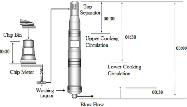
The data used in this work were collected from a eucalyptus Kraft pulp continuous digester, as indicated in Figure 1. The equipment under study is a Kamyr single vessel vapor phase digester using the Extended

Modified Continuous Cooking EMCC process (Sixta,

2006), from a market pulp mill of 500,000 air dried metric tons (admt)/year capacity, located in Minas Gerais state in Brazil.

Considering the author's experience working with the process control of this pulp mill, seventeen

process variables that influence the delignification

reactions were selected, which are: chip bulk density, chip consistency, chip bin retention time, chip bin temperature, chip meter speed, liquor/wood

relation, effective alkaline charge, sulfidity, top

digester temperature, top digester pressure, upper cooking screen alkali concentration, upper cooking screen temperature, lower cooking screen alkali concentration, lower cooking screen temperature,

lower extraction percentual flow, washing liquor flow/

chip speed relation and previous kappa number.

Next, these variables were properly adjusted according to the retention time delay as presented in Figure 1. To exemplify this adjustment, a chip sample collected at 00:00 (hh:min) at the chip bin conveyor entrance is compared to a kappa number measured in a sample collected from the blow digester at 03:30 (hh:min). A temperature at the top of the digester (and others located in the top digester) is compared to the kappa number measured in a sample collected from the blow-line digester at 03:00h later and so forth.

Initially, data samples containing missing data, dubious values, and evident outliers were removed, as well those below 50% of the normal running production. All the process data are relative to 30 minutes frequency, and were obtained from the DCS (Digital Control System). The kappa number

data were obtained from an on-line kappa number analyzer (KappaQ_{- supplied by Metso Automation),}

which uses an automatic sample collecting system and makes analysis by optical properties using a previous calibration curve.

The working dataset was divided into two independent groups (months of January and February).

The first one (with 1471 observations) was used as reference for model identification, that is, to estimate

the model parameters, whereas the second (with 1343 observations) was used to verify the generalized

forecasting capacity of the previously identified

models.

A variable selection process helps to decrease the

risk of overfitting the model by reducing the number

of independent variables in the model. This task is also important when identifying neural models since redundant variables may worsen its general performance. Besides, one consideration in the choice of predictor variables is the extent to which a chosen variable contributes to reducing the remaining variation in the response after allowance is made for the contributions of other predictor variables that have tentatively been included in the model. Other considerations include the importance of the variable as a causal agent in the process under analysis; the degree to which observations on the variable can be obtained more accurately, or quickly, or economically than those on competing variables; and the degree to which the variable can be controlled (Kutner et al., 2005). Therefore, the stepwise method was carried out

in order to eliminate variables that do not affect the kappa number significantly, with significance levels α

of 0.1 for both variable inclusion and removal (Correia

et al., 2014). As a result, 11 independent variables were selected as variable inputs to the MLR (a linear model)

and ANN (nonlinear model), as used in different

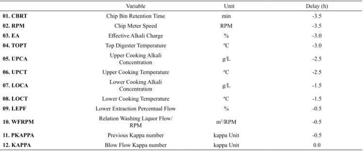
approaches (Heiat, 2002; Couto, 2009; May et al., 2011). The variable subset is listed in Table 1, with the respective time delays in relation to the dependent variable kappa number (output).

As described above, because SES and ARIMA are univariate models, the process variables from Table 1 were not used in such analyses.

RESULTS AND DISCUSSION

Due to confidentiality reasons, the kappa number

dataset was standardized, i.e., auto scaled to unit variance and mean centered, according to Equation 4

(Johnson and Wichern, 2002):

(4)

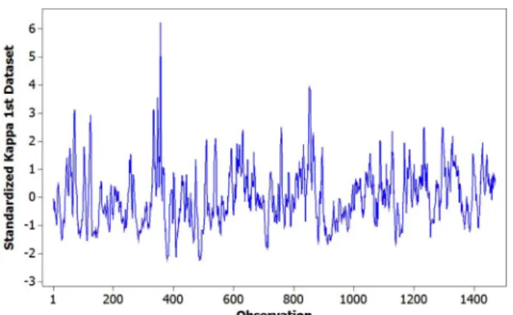
Figure 2 presents the time series evolution from the

first dataset (used for modeling), and Figure 3 presents

the time series evolution from the second dataset (used to test generalization capacity). In Figure 2 there are some long peaks around observations 350 and 850, while in Figure 3 they are present around observations 380 and 820. These peaks occurred due to wood density variations.

Both figures indicate that the proposed empirical

models were validated within the range for which they were estimated (without extrapolations) and the kappa number results have a similar behavior over time. These datasets represent major time operation characteristics.

Table 1. Digester Selected Variables.

Variable Unit Delay (h)

01. CBRT Chip Bin Retention Time min -3.5

02. RPM Chip Meter Speed RPM -3.5

03. EA Effective Alkali Charge % -3.0

04. TOPT Top Digester Temperature ºC -3.0

05. UPCA Upper Cooking Alkali

Concentration g/L -2.5

06. UPCT Upper Cooking Temperature ºC -2.5

07. LOCA Lower Cooking Alkali

Concentration g/L -1.5

08. LOCT Lower Cooking Temperature ºC -1.5

09. LEPF Lower Extraction Percentual Flow % -0.5

10. WFRPM Relation Washing Liquor Flow/

RPM m

3_{/RPM -0.5}

11. PKAPPA Previous Kappa number kappa Unit -0.5

12. KAPPA Blow Flow Kappa number kappa Unit 0.0

k

k

_s

k

n

k i

1

=

Single Exponential Smoothing

According to Figure 2, the industrial dataset is a non-seasonal time series exhibiting a constant

trend. Thus, the α parameter (Equation 1) was tested iteratively seeking a minimum RMSE, choosing

α=0.9 (after some trials) to be used at validation of the model. The first three average observations were used

as the initialization value. A histogram of residuals is presented in Figure 4, which presents a visual evidence of a normal distribution, with a mean around zero, but some undesirable residuals points beyond ± 4.

Figure 2. First Dataset Standardized Kappa Number Evolution.

Figure 3. Second Dataset Standardized Kappa Number Evolution.

The performance of the forecasting methodologies was calculated onto the second dataset according to Equations 5-7, where n is the number of observations:

MAD: Mean absolute deviation:

(5)

MAPE: Mean absolute percentage error:

(6)

RMSE: Root mean square error

(7)

Reliability was measured by the MAD and the MAPE. Accuracy was measured by the RMSE. A

benefit of the RMSE is that it is measured in the same

units as the original data, while its drawback is that large errors can dominate the value (Makridakis and Hibon, 1995). These forecasting indexes from the four methods are summarized in Table 5. In addition, the residuals (predicted(observed values) were also considered by means of the residuals histogram. The results for each approach are depicted in the following.

MAD

Y

_n

Y

1

=

/

-/

MAPE

Y

_n

Y

Y

observed i

1

=

/

-RMSE

Y

_n

Y

n 2

1

=

/

Q

-

V

Figure 4. Histogram of SES Model Residuals.

Multiple Linear Regression

Selected variables shown in Table 1 were used for

identification of the MLR model (Equation 2). Using the software EViews (Econometric Views v.5), OLS was applied in order to obtain a relationship between the dependent variable (kappa number) and the eleven regression variables. As a result, Table 2 indicates the estimated parameters for kappa number estimation (variables are described in Table 1).

This model was used to perform forecasting from the second dataset. The histogram of residuals is presented in Figure 5, with a visual evidence of normal distribution, with no residuals points beyond ± 4. This provides a better result of such model in comparison to the previous SES approach.

Time Series Method of Box-Jenkins

Besides indexes MAD, MAPE, and RMSE described in Equations 5-7, models were selected using others statistical decision criteria, like the Akaike Information Criterion (AIC), Schwarzs Bayesian

Criterion (SBC), Durbin-Watson (DW), and Theil Inequality Coefficient (TIC). Except for DW, a lower

Table 2. Estimated parameters for regression equation.

Variable Coefficient Std.Error p value

TOPT -0.0306 0.0082 0.000

LOCT -0.0410 0.0077 0.000

UPCT -0.0193 0.0080 0.015

UPCA -0.0524 0.0153 0.000

LOCA -0.0940 0.0094 0.000

CONSTANT 15.7238 1.5751 0.000

EA 0.0398 0.0161 0.013

LEPF 0.0092 0.0032 0.003

PKAPPA 0.8832 0.0098 0.000

WFRPM 0.0590 0.0260 0.023

CBRT -0.0177 0.0084 0.034

RPM 0.0128 0.0039 0.000

Figure 5. Histogram of MLR Residuals.

criteria. The DW metric is an error pattern indicator (if the pattern is random, the DW will be around 2).

These and related scalar measures to choose between alternative models in a class are discussed in some texts on statistics (Gujarati, 2004; Makridakis et al., 1995). The EViewsv.5 software was used to estimate the parameters for the ARIMA models and subsequent statistical analysis. Based on both the autocorrelation function (AC) and the partial correlation function

(PAC), ARMA models were identified (from

Equation 3).

As indicated in Figure 6, the correlogram of the

first dataset shows a slow continuous decay from Autocorrelation, and significant bars from Partial

Correlation until second-third order. The correlogram also indicates that the kappa number exerts a strong

influence on the next value.

Figure 6. Model Dataset Correlogram.

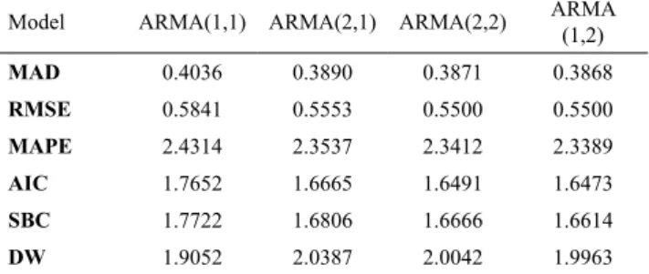
This way, ARMA (1,2), ARMA (2,1), ARMA (2,2) and ARMA (1,1) parameter subsets were tested, presenting good results (in this order) as shown in Table 3.

Table 3. Results from the statistical criteria for the selected models. Model ARMA(1,1) ARMA(2,1) ARMA(2,2) ARMA

(1,2)

MAD 0.4036 0.3890 0.3871 0.3868

RMSE 0.5841 0.5553 0.5500 0.5500

MAPE 2.4314 2.3537 2.3412 2.3389

AIC 1.7652 1.6665 1.6491 1.6473

SBC 1.7722 1.6806 1.6666 1.6614

DW 1.9052 2.0387 2.0042 1.9963

Considering accuracy and parsimony properties, ARMA (1,2) was chosen as the best forecasting model and its estimated parameters are displayed in Table 4, where C is the constant term, AR(1) the autoregressive, MA(1) and MA(2) the moving average terms.

Table 4. ARMA (1,2) model estimated parameters.

Variable Coefficient Standard Error p Value

C 16.14181 0.15600 0.000

AR (1) 0.85180 0.01552 0.000

MA (1) 0.36187 0.02742 0.000

MA (2) 0.27356 0.02699 0.000

AC and PAC functions from residuals are presented in Figure 7, indicating a white noise and homoscedasticity of residuals.

Applying the coefficients indicated in Table 4

at Equation3, the fitted model was applied to the validation data set to perform predictions. A histogram of the residuals is presented in Figure 8, which presents

no values beyond ± 3, with a significant frequency

between -1 and 1, indicating a better description

of the kappa number in comparison to the first two

Artificial Neural Networks (ANN)

Using the modeling data subset, the neural network model was constructed following the steps

of specification, selection and final model estimation.

Matlab (MATrix LABoratory) v.7.9.0 was used to estimate the ANN parameters.

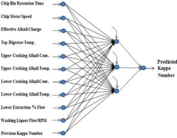
In the ANN model, the MLP architecture was used; 11 input variables (Table 1); 1 output variable (kappa number); 1 hidden layer; hyperbolic tangent as the transfer function; 750 epochs (after some trials); 75% in the training dataset; 25% in the validation dataset; Identity Output Layer Transfer Function. To select the optimum neural network model, the number of hidden neurons was varied from 1 up to 23 (each value ran

30 times), according to the correlation coefficient,

RMSE (Root Mean Squared Error), angular and linear

coefficient. The average degree of association between

collected and estimated kappa number was calculated on the validation data subset. Figure 9 summarizes

results of correlation coefficient (where the vertical bar means the average confidence interval) from 1 to

23 hidden neurons. The selected model was the one containing three hidden neurons.

A re-estimation of the weights matrix for the ANN model, using both the training and the validation

datasets, was carried out. Figure 10 depicts the final

neural network model with eleven inputs and three hidden neurons.

Figure 7. ARMA (1,2) Residuals Correlogram.

Figure 8. Histogram of ARMA (1,2) Residuals.

Figure 9. Hidden neurons evaluation.

Figure 10. Final neural network model.

The error can be determined by running all the training cases through the network, comparing the actual output generated with the desired or target outputs. The algorithm therefore progresses iteratively, through a number of epochs. In each epoch, each training case is submitted in turn to the network, and the target (collected in the mill) and actual (model estimates) outputs are compared to the error calculated. This error is used to adjust the weights, and then the

process repeats. The initial network configuration is

at random, and training usually stops when a given number of epochs elapse or when the error stops increasing.

After defining the architecture model, the second

and ARIMA), a specific algorithm was developed

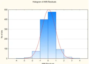
in a Matlab code to use the parameters obtained in modeling data from the validation dataset, considering that the ANN default of the software uses the same dataset for training, selection, and validation of model parameters. Thus, a conjunct of residuals (predicted-observed) was obtained, for which the histogram is indicated in Figure 11.

scope of the present study, could be used to determine

the influence of the inputs over the output kappa

number.

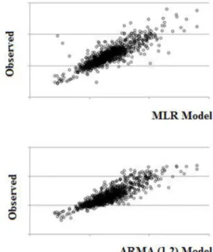
Complementing the results, Figure 12 illustrates the modeled versus observed values for all the methods

(for confidentiality reasons the axis data are omitted).

In a general way, setting aside SES (the simplest), all the methods present good accuracy. Moreover, ARIMA showed better values in all forecast indexes. Likewise, more than 90% of the prediction data is lower than 01 kappa unit of deviation in the ARIMA

model, confirming it to be the best option among the

analyzed models.

CONCLUSIONS

This paper discusses kappa number estimation

using different modeling approaches in a continuous

cooking process. Data from an industrial continuous digester were used to compare the performance of

these kappa number predicting methods. Four different

methods were compared considering accuracy of the results. SES and ARIMA methodology were developed in dynamic models using the observed and predicted kappa number values. MLRA and ANN Models were done with 11 process input cooking variables. Considering that none of the data points included in the validation subset were used in the training phase, it is possible to conclude that the ANN, MLR and ARIMA models are quite acceptable considering practical application in predicting kappa number, providing digester operators with an accurate on-line estimation to be used as an inferential sensor. These models presented a desirable normal distribution with zero mean in residuals. Considering the results obtained in this study, the ARIMA model showed better accuracy when compared to the others, according to all statistical forecasting indexes evaluated, followed by MLR,

ANN and SES. With these measurements it is possible

to estimate the blow-line kappa number before the end of the cooking process, allowing the operating personnel to make faster corrections concerning kappa number deviations. ARIMA methodology may be a useful tool for pulp mills, since it can be applied to optimize and control the cooking process and may be easily included in any electronic spreadsheet, updated from time to time as more data become available.

These four methods can be adapted to any continuous reactor, turning this manuscript of interest for the pulp and paper industry audience and for

different chemical industries as well.

Figure 11. Histogram of ANN residuals.

Table 5 summarizes some forecasting indexes from the four methods studied, as expressed in Equations 5, 6 and 7. Also included is the percentage of absolute deviation value lower than 1 kappa unit (which is considered an acceptable value for mill applications).

Table 5. Summary of Forecasting Indexes.

MODEL SES ARIMA MLR ANN MAD 1.0261 0.4552 0.5540 0.6150 MAD<1

(%) 64.1102 90.7713 86.0883 81.7216 RMSE 1.4052 0.4130 0.7681 0.8549 MAPE 6.2220 2.7327 3.3373 3.6740

Figure 12. Modeled versus Observed Kappa Number.

NOMENCLATURE

ANN Artificial Neural Networks

ARIMA Auto Regressive Integrated Moving

Average

ARMA Auto Regressive Moving Average

MLR Multiple Linear Regression

SES Single Exponential Smoothing

α weighted index

β₀, β₁...β_q regression estimated parameters

(1 i);

i p

1

d=n - z

=

/

ε_t error component (Yt-Ŷt), with mean =

0; variance = σ2

ϕ₁,...,ϕ_p the parameters of the AR model;

θ₁,...,θ_q the parameters of the MA model;

k_i kappa number observation

k_s standardized kappa number

k kappa number mean

S_k kappa number standard deviation

n total number of the sample

x₁, x₂...x_q correlated variables

Y_t observed value at time t

Ŷ_t estimated value at time t

_

REFERENCES

Adhikari, R. and Agrawal, R. K. An Introductory Study on Time Series Modelling and Forecasting, Germany, LAP LAMBERT Academic Publishing (2013).

Ahvenlampi, T., and Kortela, U., Clustering algorithms in process monitoring and control application to continuous digesters, Informatica, 29, 101-109 (2005).

Araneda, F. J., Melo, D. L., and Canales, E. R. Industrial Lo-Solids pulp digester simulation by the Purdue model, TAPPI Journal, 8(4), 4-9 (2009). Assidjo, E., Yao, B., Kisselmina, K. and Amane,

D., Modeling of an industrial drying process by

artificial neural networks. Braz. J. Chem. Eng.,

25 (3), 515-522 (2008). DOI:10.1590/S0104-66322008000300009

Badwe, A., Continuous Digester Optimization using Advanced Process Control. In: Procedings Computer Society of India (2016).

Balasko, B., and Abonyi, J., What happens to

process data in chemical industry? From source to applications - an overview. Hungarian Journal of Industrial Chemistry Veszprem, 35, 75-84 (2007). Blackburn, R., Lurz, K,Priese, B., Gob, R. and Darkow,

Box, G., and Jenkins, G., Time series analysis: Forecasting and control, 2nd _{ed, San Francisco:}

Holden-Day (1976).

Bowerman, B. L., O'Connell, R. T., and Koehler, A. B., Forecasting, time series, and regression: an applied approach 4th _{ed, Duxbury Press, Belmont,}

USA (2005).

Chase Jr., C.D., Demand-Driven Forecasting: A Structured Approach to Forecasting, 2nded., Wiley

and SAS Business Series (2013).

Correia, F. M., Mingoti, S. A., and D'Angelo, J. V. H., Predição do número kappa de um digestor contínuo de celulose kraft usando análise de regressão

múltipla. In:Anais do XX COBEQ, Blucher

Chemical Engineering Proceedings, 1(2), 11845-11852. São Paulo, Brazil, (2014). DOI 10.5151/ chemeng-cobeq2014-0928-22370-148607

Costa, M. M., and Colodette, J. L., The impact of kappa number composition on eucalyptus kraft pulp bleachability. Braz. J. Chem. Eng., 24(1), 61-71 (2007).

Couto, M.P. C., Review of input determination techniques for neural network models based on mutual information and genetic algorithms, Neural Computing and Applications, 18(8), 891 (2009). Danese, P., and Kalchschmidt, M., The role of the

forecasting process in improving forecast accuracy and operational performance, International Journal of Production Economics, 131, 204-214 (2011). Dahlquist, E., Process simulation for pulp and paper

industries: Current practice and future trend. Chemical Product and Process Modeling, 3(1), 18 (2008). DOI: 10.2202/1934-2659.1087

Draper, N.R., and Smith, H., Applied Regression Analysis, 3th ed, John Wiley & Sons, USA (1998).

Dufour, P., Bhartiya, S., Dhurjati, P.S., and Doyle III, F.J., Neural network-based software sensor: Data set design and application to a continuous pulp digester, Control Engineering Practice, 13(2), 135-143 (2005).

Fox, J., Applied regression analysis, linear models, and related methods. Sage Publications, Thousand Oaks, USA (1997).

Fung, C.A., George Box, quality, and improving almost anything. Applied Stochastic Models in Business and Industry, 30(1), 71-79 (2014).

Galicia, H. J., He, Q. P., and Wang, J., Adaptive Kappa

Number Prediction via Reduced-Order Dynamic PLS Soft Sensor for the Control of a Continuous Kamyr Digester, Tappi PaperCon Conference (2012).

Germgård, U., The Arrhenius Equation is Still a Useful Tool in Chemical Engineering, Nordic Pulp

& Paper Research Journal, 32(1), 21-24 (2017).

DOI 10.3183/NPPRJ-2017-32-01-p021-024

Gullichsen J., andFogelholm, C.J., Chemical

engineering principles of fiber line operations.

In Chemical Pulping., Papermaking Science and Technology, Book 6A. Fapet Oy, Jyvaskya, Finland, 244-327 (2000).

Gujarati, D. N., Basic Econometrics. NY: The McGraw-Hill 4th_{ed. 536-540 (2004).}

Hair, J. Anderson, R., and Babin, B., Multivariate Data Analysis. Prentice Hall, 7th _{ed. (2009).}

Halmevaara, K., Simulation Assisted Performance Optimization of Large-Scale Multiparameter Technical Systems. Ph.D. Thesis. Helsinki University of Technology, Finland (2009).

Hart, P. W. E., Enhancing yield through high-kappa

pulping. Tappi Journal, 13(10), 33-35 (2014). Haykin, S., Neural Networks: A Comprehensive

Foundation. Macmillan Publishing Company, New York (1994).

Heiat, A., Comparison of artificial neural network

and regression models for estimating software

development effort, Information and Software

Technology, 44, 911-922 (2002).

Hill, W.J., George Box: His interface with industry and

its impact. Applied Stochastic Models in Business and Industry, 30(1), 11-19 (2014).

Himmelblau, D.M., Applications of artificial neural

networks in chemical engineering, Korean Journal of Chemical Engineering, 17(4), 373-392 (2000). DOI:10.1007/BF02706848

Holt, C.C., Forecasting seasonals and trends by exponentially weighted moving averages. International Journal of Forecasting, 20(1), 5-10 (2004).

Hornik, K., Stinchcombe, M., and White, H.,

Multilayer Feedforward Networks are Universal Approximators. Neural Networks, 2, 359-366 (1989). DOI: 10.1016/0893-6080(89)90020-8

Johnson, R. A., and Wichern, D.W., Applied

multivariate statistical analysis. 5th _{ed. New Jersey:}

Prentice Hall (2002).

Khashei, M., and Bijari, M., A novel hybridization of

artificial neural networks and ARIMA models for

time series forecasting, Applied Soft Computing, 11, 2664-2675 (2011).

SnO₂ Nanofluid via Statistical Method and an

Aritificial Neural Network. Braz. J. Chem. Eng.

32(4), 930-917 (2015). DOI: 10.1590/0104-6632.20150324s00003518

Kocurek, M. J., Grace, T. M., and Malcolm, E., Alkaline Pulping. TAPPI/CPPA, Atlanta, v. 5 (1989).

Kutner, M., Nachtsheim, C., Neter, J., and Li, W.,

Applied Linear Statistical Models, McGraw-Hill/ Irwin, 5th _{ed., USA (2005).}

Laakso S., Modeling of Chip Bed Packing in a Continuous Kraft Cooking Digester. Ph.D. Thesis, Helsinki University of Technology, Finland (2008). Lindstrom, M., Challenges in kraft cooking of

Eucalyptus. In:Proceedings. 3º ICEP-International Colloquium on Eucalyptus Pulp, 1-4 (2007). MacLeod, M., The top ten factors in Kraft pulp yield.

Peperi ja Puu, 89(4), 1-7 (2007).

Makridakis, S. G., and Hibon, M., Evaluating

Accuracy (Or Error) Measures. INSEAD Working

Papers Series. Fontainebleau, France (1995).

Makridakis, S.G., Wheelwright, S.C., and McGee,

V. E., Forecasting Methods and Applications, In

Wiley Series in management. 2nd Edition, John Wiley & Sons, USA (1983).

May, R., Dandy, G., and Maier, H., Review of input

variable selection methods for artificial neural

networks. INTECH Publisher, (2011).

Monrroy, M., Mendonça, R., Baeza, J., Ruiz, J., Ferraz, A., and Freer, J., Estimation of Hexenuronic Acids and Kappa Number in Kraft Pulps of Eucalyptus Globulus by Fourier Transform near Infrared Spectroscopy and Multivariate Analysis, Journal of Near Infrared Spectroscopy, 16(2), 121-128 (2008). Moral, A., Cabeza, E., Aguado, R., and Tijero, A., NIRS Characterization of Paper Pulps to Predict Kappa Number, Journal of Spectroscopy, 2015, article ID 104609 (2015). DOI: 10.1155/2015/104609

Ng, Y.S., and Srinivasan, R., Data mining for chemical process industry. In: John Wang (Ed.),

Encyclopedia of Data Warehousing and Mining. 2nd

ed., 458-464, IGI Global, PA, USA, (2009). Pankratz, A., Forecasting with Univariate Box-Jenkins

Models: Concepts and Cases. Inc., Hoboken, NJ, EUA(2008). DOI: 10.1002/9780470316566

Patterson, D., Artificial Neural Networks. Singapore:

Prentice Hall (1996).

Pikka, O., and Andrade, M.A., New developments in pulping technology. 7th _{ICEP-International}

Colloquium on Eucalyptus Pulp, Vitoria, Brazil, 1-4 (2015).

Rahman, M., Avelin, A., Kyprianidis, K., and Dahlquist, E., An Approach For Feedforward Model Predictive Control For Pulp and Paper Applications:

Challenges And The Way Forward. In: Proceedings, TAPPI Papercon, v 10, Minneapolis, USA, (2017). Rantanen, R., Modelling and Control of Cooking

Degree in Conventional and Modified Continuous

Pulping Processes, Ph.D. Thesis. Faculty of Technology, University of Oulu, Finland (2006). Ryan, T.P., Statistical Methods forQuality

Improvement. 407-434, Wiley and Sons, 3rd _ed.

NY, (2011).

Santos, A., Anjos, O., Simões, R., Rodrigues, J., and Pereira, H., Kappa Number Prediction of Acacia melanoxylon Unbleached Kraft Pulps using NIR-PLSR Models with a Narrow Interval of Variation. BioResources, North America (2014). Available at: http://ojs.cnr.ncsu.edu/index.php/BioRes/ article/view/BioRes_09_4_6735_Santos_Kappa_ Prediction_Acacia_Kraft.Accessed: 23 May. 2016. Saavedra, A.D.M., Implementacion y modelamiento

predictive de coccion downflow lo-solid en

digestor continuo. MSc Thesis, Federal University of Viçosa, Brazil (2011).

Smook, G.A., Handbook for Pulp and Paper Technologists, 2nd ed. Angus Wilde Publications,

Vancouver, (1992).

Sixta, H., Handbook of Pulp. WILEY-VCH Verlag GmbH &Co. (2006).

Sixta, H., and Rutkowska, E.W., Comprehensive

kinetic study on kraft pulping of Eucalyptus

globulus. Part 1: Delignification and degradation of

carbohydrates, O Papel, 68(2), 54-67 (2007).

Weding, H., Aspects of extended impregnation kraft