Can investors profit from mutual funds performance persistence?

Can Investors Profit from Mutual Funds Performance Persistence?

Pedro Fezas Vital

152413001

Abstract

We use almost 21,000 equity mutual funds worldwide returns to provide evidence that investors can make significant profits if they invest in persistence strategies. Our regressions results are mixed and show some funds managers are better in picking stocks. We show that investors would have been delivered Annualized Sharpe Ratios up to 0.81. We also test our strategies under different economic environments and conclude that in expansion periods, our strategies outperform both S&P500 and MSCI. We also find our results still hold after deducting funds’ redemption fees, especially for holding periods longer than 3 months.

Supervisor: Professor José Faias

Dissertation submitted in partial fulfilment of requirements for the degree of Master of Science in Finance, at Universidade Católica Portuguesa, September 2015

i

Acknowledgments

I am very grateful to several different people. I am using this space to make sure all of them are mentioned.

Firstly, I would like Professor José Faias for all the time he spent helping me going through the process of completing this thesis.

Secondly, but surely more important, I want to thank my parents and my family for all the support they gave during my life. I want not only to thank them but also to dedicate this thesis to them.

I want also to mention my friends, with whom I experienced most of the best and worst moments of my life. I also want to thank Fundação para a Ciência e Tecnologia

ii

Table of Contents

I. Introduction ... 1

II. Data & Methodology ... 4

III. Investment Strategy ... 12

IV. Results ... 15

V. Redemption Fees ... 29

VI. Conclusions and Further Research ... 29

iii

Index of Tables

Table I: Returns Serial Correlation ... 6

Table II: Summary Statistics ... 7

Table III: Regression Coefficients ... 11

Table IV: Strategy based on Past Returns Results ... 17

Table V: Strategy based on Past Sharpe Ratio... 20

Table VI: Strategy based on Past Certainty Equivalent ... 21

Table VI: Performance vs Passive Benchmarks ... 28

Index of Figures Figure I: Investment Strategy ... 11

Figure II: Investment Strategy with Different Estimation Periods ... 24

Figure III: Investment Strategy Results with Different Criteria ... 25

1

I. Introduction

The Efficient Market Hypothesis (EMH) claims that, in strong-form efficient markets, all the information related to the effects of future events in stocks’ prices is already incorporated in today’s price (Roberts, 1967). In Fama’s (1970) words, efficient markets are those in which “prices always ‘fully reflect’ available information”. According to the EMH, returns should, therefore, be unpredictable, at least in strong-form efficient markets. Changes in securities’ prices should only be attributable to new information that no one was aware of. In that sense, researchers should only study which factors explain prices’ changes. Trying to predict securities’ returns should be pointless. However, not everything is explained by the Efficient Market Hypothesis. Two major unanswered questions arise from EMH. The first one is what can be considered “all available information”. The second is how can one measure or ensure that all information is already reflected in securities prices.

The fact that there are no clear answers for both questions has led to several studies on investment strategies profitability and returns’ predictability. As far as we know, we use the biggest mutual fund sample to study whether or not returns are predictable and if investors can make profits taking into account the fact that returns do present some degree of predictability. Moreover, we implement almost 400 persistence strategies using ranking criteria we did not find in previous studies.

In Campbell and Shiller (1998), the authors use Vector Autoregressive Models (VAR) and conclude log dividend price ratios do have predictive power over future discount rates, and therefore, future stock prices. These results are supported by those of Fama and French (1988), who conclude not only dividend yields do predict future stock prices, but also that predictive power increases with return horizon. Hodrick (1992) uses VAR models and states these tests “provide strong evidence of the predictive power of one-month-ahead returns at least for the sample from 1952 to 1987”. Predictability in stock returns is studied in several different ways. In Gencay (1998), the author finds nonlinear predictability in stock market returns, when conducting a study based on the performance of technical analysis strategies. However, consensus on returns predictability is not easy to find. Even assuming Goyal and Welch (2008) proposition that there is some publication bias in favor of significant results, one can find some studies that found there is, at most, little prediction power of prices and returns. In Stambaugh (1999), the author states regressions some authors use to study returns predictability deliver up warded biased results and when corrections are made, results tend to

2 become insignificant. Goyal and Welch (2008) conduct a study in which previously used models are reviewed and find no robust returns’ predictor. Moreover, they claim prediction power erodes over time. Ang and Bekaert (2007) results contradict those of Fama and French (1988), since they claim that, even though dividend yields have some predictive power in the short-term, it disappears in the long-term.

Every actively managed investment strategy relies on the assumption that future prices are, at some level, predictable. The hardest challenge has ever been to discover what drives returns. In the literature one can find some examples of market anomalies that can help investors to make extra profits. Anomalies are from now on defined as events that allow investors to make additional profits without bearing huge extra levels of risk and happen repeatedly. In Rozeff and Kinney (1976), authors found New York Stock Exchange returns are seasonal and tend to be higher in January. This anomaly is now commonly mentioned as the January effect and is sometimes explained by the willingness to pay less tax. When analyzing daily returns of American Stocks, French (1980) reported negative average returns on Mondays and positive in all the other four days of the week. French’s (1980) are supported by those of Agrawal and Tandon (1994), in which five seasonal effects are studied. In their paper, the authors find significant negative returns on Mondays in nine countries. As in many other Finance related fields, consensus does not exist. In Steeley (2001) is concluded that, at least for the UK, the weekend effect disappears during the 1990’s. Other effects were identified throughout the years. Harris and Gurel (1986) conduct a study to understand whether or not stock additions to the Standard & Poor’s Index have an impact on shareholders wealth. In their study, the authors conclude additions may cause a significant increase in securities prices up to 3 percent, due to shifts in demand. These results are in accordance with those of Shleifer (1986) which states stocks to be added to the Standard & Poor’s earned a positive and significant abnormal return at the announcement date. Moreover, stock returns are persistent up to 10 days. There are other market anomalies. We do not mention all of them in this thesis. Examples of anomalies are given because it is our intention to study the existence of one additional anomaly and to understand if investors can profitably exploit such anomaly. One of EMH implications is that it should be indifferent to invest money in actively or passively managed strategies, since, at least in strong-form efficient markets, all available information is already incorporated in today’s securities prices. As shown before, there are several market anomalies that may imply EMH, in some moments, does not hold. In this thesis, we use mutual funds to study the existence of equity mutual funds managers’ ability to

3 pick stocks and beat benchmarks. In order to do so, we want to take advantage of returns persistence, measured by serial correlation. Once again, consensus does not exist. Whereas Lo and Mackinlay (1988) find positive serial correlation in weekly and monthly returns Jegadeesh (1990) report negative and highly significant serial correlation in stocks’ monthly returns and positive for longer lags. In this thesis, we intent to study serial correlation of equity mutual funds returns’ and, if possible, implement investment strategies that take advantage of such feature.

If EMH and its implications are true, it is arguable that persistence strategies in mutual funds should not deliver investors any abnormal return, or positive alpha. However, amongst other authors, Grinblatt and Titman (1992) found a relationship between past and future performance of mutual funds. The authors clearly state “we can assert that the past performance of a fund provides useful information for investors who are considering an investment in mutual funds”. Hendricks et. al. (1993) provides evidence of returns’ persistence in mutual funds, especially in the short term, when analyzing a sample of quarterly returns of mutual funds, during the period of 1974-88. Performance persistence is, however, not consensual. Even though some authors state it exists, one can also find several studies arguing there is no benefit in using past performance as predictor of future returns. Jensen (1969) found no evidence of a relevant relationship between past and future performance of mutual funds and therefore claims that “mutual funds managers on the average are unable to forecast future security prices”. In Fama and French (2010), the authors conclude that if there is any stock picking ability in funds managers to generate “benchmark-adjusted expected returns that cover costs, their tracks are hidden in the aggregate results by the performance of managers with insufficient skill”. Therefore, authors found no evidence of the possibility of investors taking advantage of the skills of funds managers.

In this thesis, it is our intention to study the presence of funds managers “stock picking” ability. Even though it is not the main concern of this thesis, our final results have also an implication on the Efficient Market Hypothesis. In order to reach conclusions about managers’ ability to outperform benchmarks and shed some additional light on the existence of managers’ skill to pick stocks, we build portfolios based on the past performance of almost 21,000 equity mutual funds, operating worldwide. It is of major importance to state that we do not invest in momentum strategies. Whereas, very often, momentum strategies are zero-investment strategies in which investors buy past winners and sell past losers, we focus only

4 on the long leg of these types of strategies. Therefore, we do not study momentum, but persistence. Developing and implementing persistence investment strategies and reporting their results, measured by Annualized Returns, Sharpe Ratio or Certainty Equivalent has some advantages. Firstly, final results can be easily understood not only by researchers, but also by practitioners, due to the statistical simplicity of the portfolios’ performance measures and building criteria. Secondly, we use funds from all over the world, which differ from most studies that focus in funds developing their activity and implementing investment strategies in specific countries or regions. Two main features of the strategies we use in this article should be noticed by both private investors and funds’ managers. Whereas implementation easiness can be very useful to private investors, simplicity can be used by funds’ managers to collect more money and therefore increase Assets Under Management (AUM) and thus, funds’ size. In this thesis, we use a sample of almost 21,000 equity mutual funds operating worldwide in order to test whether or not investors can profit from using past performance as unique criteria to invest in mutual funds. We build nine different clusters in order to understand if there are significant differences in performance. We are able to state that, as in Hendricks et. al. (1993), mutual funds returns are persistence in the very-short term. On the other hand, we also claim that, in accordance with DeBondt and Thaler (1985), returns tend to revert in the long-term, as we demonstrate further in this thesis. We then rank funds based on three main performance measures: Past Returns, Sharpe Ratio and Certainty Equivalent. We find some funds’ managers are better in picking stocks. For the others, our results are the same as Fama and French (2010), since we do not find any reason to claim funds managers do have stock picking ability. However, after building portfolios of funds and measuring their performance, we conclude investors could have been granted returns of 35.0% per year and Annualized Sharpe Ratios of up to 0.81. We are also able to claim investing in our strategies would be extremely risky, which is explained by Annualized Standard Deviation that can reach a value of 46.00%

This thesis continues as follows: in Section II, we present the data and methodology we used to pursue our final objective. Section III describes the mechanics of our investment strategies. In Section IV, one can find the results our strategies deliver to investors, without taking into account redemption fees. In Section V, we show the impact of redemption fees in our portfolios and Section VI concludes.

5

II. Data & Methodology

In order to study the existence of stock picking ability, we use a sample of 20,879 equity mutual funds operating worldwide. Monthly prices were drawn from the Lipper Database, from January 1991 to December of 2014 and raw returns were calculated. According to Carhart (1997), there might be some selection bias when one uses Lipper’s data set, since it includes less 100 mutual funds per year than other databases. However, in Malkiel (1995), the author uses the previously mentioned data set and found almost the same mean mutual funds return as Carhart (1997). Hence, one may argue selection bias should not be a major concern when using Lipper Database. Moreover, by using data from 1991 onwards, we correct for the bias mentioned by Carhart (1997). The same should not be claimed about survivorship bias. Malkiel (1995) states survivorship bias may be very relevant not only because today’s investors do not pay attention to returns of funds that already ceased operations but also due to the fact that “commonly used data sets of mutual fund returns typically show the past records of all funds currently in existence”. Since the information contained in the returns of dead funds might be relevant to the analysis, it is of major importance to include in the sample the returns of mutual funds that, for any reason, ceased operations and are currently not reporting any returns. By using Lipper Database, that contains information of past returns of already dead mutual funds we eliminate the survivorship bias problem and the consequences it could have in our analysis.

Since we assume the possibility of finding differences across funds, we start by clustering the mutual funds following three main criteria: type of asset invested – Small & Mid and Large Caps; Geographical focus – European, Emerging Markets, Global, Japan and North American Funds – and Sector Funds, from now on considered the funds within the sample that only invest in equities of companies which operate in specific sectors. In the end, nine different categories were taken into account in this thesis, since we also considered an All Equity Funds cluster, which comprises all the 20,879 mutual funds.

One way one can use to study the existence of funds’ managers stock picking ability is to test whether or not funds returns are persistent in time. If so, there might be some room for claiming funds’ returns have a certain degree of predictability. In this thesis, we measure persistence by the lagged serial correlation of funds’ returns. In order to compute returns’ serial correlation, we start by creating an Equally Weighted Index (EW) with every available

6 fund in each period and compute its return. Afterwards, we calculate the serial correlation of returns of each cluster EW, for 1 to 12-month lags.

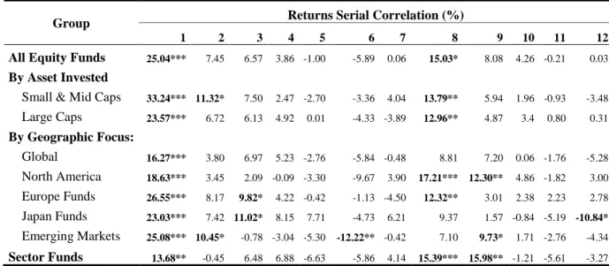
Table I. Returns Serial Correlation

Serial correlation of returns for all the previously constructed clusters can be seen in this Table. We consider returns’ autocorrelation evidence of persistence and show coefficients for the 1 to 12-month lagged serial correlation of returns. The 1%, 5% and 10% statistical significance levels are denoted by the symbols***,** and *, respectively.

Group Returns Serial Correlation (%)

1 2 3 4 5 6 7 8 9 10 11 12

All Equity Funds 25.04*** 7.45 6.57 3.86 -1.00 -5.89 0.06 15.03* 8.08 4.26 -0.21 0.03

By Asset Invested

Small & Mid Caps 33.24*** 11.32* 7.50 2.47 -2.70 -3.36 4.04 13.79** 5.94 1.96 -0.93 -3.48

Large Caps 23.57*** 6.72 6.13 4.92 0.01 -4.33 -3.89 12.96** 4.87 3.4 0.80 0.31 By Geographic Focus: Global 16.27*** 3.80 6.97 5.23 -2.76 -5.84 -0.48 8.81 7.20 0.06 -1.76 -5.28 North America 18.63*** 3.45 2.09 -0.09 -3.30 -9.67 3.90 17.21*** 12.30** 4.86 -1.82 3.00 Europe Funds 26.55*** 8.17 9.82* 4.22 -0.42 -1.13 -4.50 12.32** 3.01 2.38 2.23 2.78 Japan Funds 23.03*** 7.42 11.02* 8.15 7.71 -4.73 6.21 9.37 1.57 -0.84 -5.19 -10.84* Emerging Markets 25.08*** 10.45* -0.78 -3.04 -5.30 -12.22** -0.42 7.10 9.73* 1.71 -2.76 -4.34 Sector Funds 13.68** -0.45 6.48 6.88 -6.63 -5.86 4.14 15.39*** 15.98** -1.21 -5.61 -3.27

In Table I, we present the lagged serial correlation of funds’ returns, by cluster and number of lags, in months. We find clear evidence of persistence in returns, measured by the significant lagged serial correlation, especially in the very short term. For all the clusters, the 1 month lagged autocorrelation is positive and significant at the one percent level, which implies that the last month return has a positive influence on the following month return. In that sense, our results are accordance with those of Grinblatt and Titman (1992), who state past returns do contain information about future performance. Our results do also support Lo and Mackinlay (1988) claim that returns are persistent in time and present positive serial correlation in the short term. Whereas the higher values of serial correlation can be found in the Small & Mid Caps (33.24%), European Funds (26.55%) and Emerging Markets (25.08%) funds’ clusters, funds included in the Sector funds’ cluster present the lowest level of 1 month serial correlation (13.68%), which may be explained by the appearance of new funds that invest in economic sectors that already existing funds disregard. Despite the fact that most of the clusters’ returns tend to stop being significant at the 4-month lag, there is room to argue that, in most of the clusters, returns are persistent up to 8 months However, it is also possible to argue that persistence in returns tends to become negative in with time, what can be seen by

7 the negative values in the 12-lagged coefficients we show in Table I, which may indicate returns tend to mean revert in the longer term. Longer term mean reversal is shown is DeBondt and Thaler (1985), who show past losers tend to perform better than past winners, in the mid-term. Positive and significant serial correlation may lead to the conclusion that returns might have some degree of predictability.

In this thesis, we intend not only to provide evidence on the ability of funds’ managers to pick stocks but also to evaluate the performance of a strategy in which the main investment criteria is the past performance of funds. Therefore, we try to make this thesis useful for both researchers and investors by conducting a study about the existence of a specific skill and to assess the possibility of taking advantage of such skill. In order to proceed, we computed and show summary statistics for the returns of the EW indices we built in every cluster we mentioned before. Measures like Annualized Mean Returns, Standard Deviation, Annualized Sharpe Ratio and Certainty Equivalent are shown in Table II.

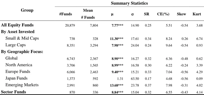
Table II. Summary Statistics

Summary Statistics for all the clusters we mention previously are shown in this table. #Funds stands for the total number of funds within each cluster. Mean #Funds is considered the average number of funds during the sampling period from January 1991 to December 2014. µ is the annualized average return of each cluster and the annualized standard deviation of returns is represented by . SR represents the average annualized Sharpe Ratio delivered by the EW and CE the Certainty Equivalent for a power-utility function with a risk aversion coefficient equal to 2. Skew and Kurt stand for Skewness and Kurtosis of the returns’ distributions. The 1%, 5% and 10% statistical significance levels are denoted by the symbols***,** and *, respectively.

Group

Summary Statistics

#Funds

Mean

µ  SR CE(%) Skew Kurt

# Funds

All Equity Funds 20,879 7,804 7.77*** 14.90 0.25 5.51 -0.54 3.68

By Asset Invested

Small & Mid Caps 738 328 11.30*** 17.61 0.34 8.24 0.26 6.74

Large Caps 8,351 3,294 7.98*** 24.04 0.24 9.64 -0.54 0.93 By Geographic Focus: Global 6,743 2,367 8.90*** 16.27 0.32 6.36 -0.48 0.62 North America 3,706 1,565 8.99*** 16.58 0.30 6.22 -0.24 3.39 Europe Funds 6,066 2,463 9.40*** 15.21 0.33 7.04 -0.56 4.29 Japan Funds 1,373 592 1.31 63.50 0.17 4.68 -0.56 0.09 Emerging Markets 2,991 860 13.68*** 23.78 0.37 7.98 -0.31 4.02 Sector Funds 870 336 8.84*** 15.04 0.32 6.55 -0.43 4.14

8 As mentioned before, our sample consists of 20,879 equity mutual funds worldwide with a minimum of 24 observations of monthly returns, which we computed based on the prices we extracted from Lipper’s Database, from the period starting in January, 1991 to December of 2014. Within the sample, one can find funds with a maximum of 289 returns’ observations. In total, our sample comprises 2,251,980 observations of funds’ monthly returns and the average number of observations per fund is 107. One of the first conclusions one can draw when analyzing Table II is that the number of funds in the All Equity funds cluster is not equal to the sum of funds that invest in Small & Mid Caps and Large Caps, which is explained by the fact that not every fund invests exclusively in equities based on this criteria.

As stated before, we include in our sample both live and dead funds. We do that in order to avoid survivorship bias, which could make our results better without any relevant reason. Within the sample are 1,598 mutual funds that, for any reason, do not report information about prices anymore. All those funds were considered dead and represent almost 8% of the total funds in the sample. Almost 40% of the funds included in the sample invest exclusively in equities of large companies. After dividing the funds by geographical focus of their investment strategy, we observe that most part of the funds invested in Global or European equities. Table II also provides information on annualized returns of funds’ investments. If one decided to invest in an EW index of funds, she would almost surely be delivered positive and significant returns year after year. Positive and significant returns range from 7.77% in the All Equity Funds cluster to 13.68% in Emerging Markets. Even though returns are high, risk is also very high when investing in mutual funds. At his point, we measure risk by the Annualized Standard Deviation of returns. Investors would opt for the least risky cluster if they invested in the All Equity Funds cluster (14.90%) and would have carried the largest amount of risk if they allocated wealth to the Japan Funds cluster (63.5%). These levels of risk are easily explainable. Geographical diversification of the funds included in the All Equity Funds cluster implies a lower exposure to some types of risks, which ultimately causes a lower level of risk. The Japanese cluster is quite different. During the sampling period, Japan faced, at least, two major economic crises and some expansion periods, which helps explaining the very high Annualized Standard Deviation of returns. Some of our results are counter intuitive. For example, Large Caps clusters present an Annualized Standard Deviation of 24.04%, which contradicts the theory that states the higher the risk, the higher should the return be, since it delivered lower returns than the Small & Mid Caps cluster (11.30%), with higher risk. Investors would not receive any significant return only if they had decided to

9 invest in funds that invested solely in Japanese equities, which can be explained by the economic situation in Japan during the 90’s and the global economic environment from 2008 onwards. These results are positive not only due to the fact that returns are consistently positive and significant but also because there are two economic crises within the sampling period. The first one happened between 1999 and 2001and the second one started in 2008 and its effects are still felt in, at least, some economies and countries worldwide. In order to assess funds’ performance, taking into account strategies’ risk exposure; we compute Annualized Adjusted Sharpe Ratios (SR) and Certainty Equivalent (CE), which is from now on defined as the risk-free rate investors’ would demand in order to move from risky assets to those which pay the risk-free rate. Whereas SR only considers the two first moments of the returns’ distributions, CE measures take into account the impact of the Skewness and Kurtosis of the distribution. CE was calculated with an underlying assumption that utility follows a power function with a risk aversion coefficient (𝛾) of 2. The formula we use to compute CE (1) is shown below.

𝐶𝐸 = (𝑈̅ ∗ [1 −𝛾])

1

1−𝛾_{− 1 (1)}

One assumption underlying the commonly used Sharpe Ratio formula is that returns are independent and identically distributed. In our sample, returns are serially correlated. Due to that fact, we correct the value of annualize SR following Lo’s (2002) procedure. This method implies that, instead of multiplying the SR by the square root of the number of periods per year, one shall multiply the SR by the term presented in formula (2).

𝜂(𝑞) = 𝑞

√𝑞+2 ∑𝑞−1_𝑘=1(𝑞−𝑘)∗𝜌(𝑘)

(2) As suggested in Lo’s (2002), 𝜌(𝑘) is the coefficient of the (𝑞 − 𝑘)significant lagged serial

correlation. Whenever there is positive serial correlation in returns, Lo’s (2002) method has a negative impact on the Annualized Sharpe Ratio.

By observing Table II, one can conclude the minimum Adjusted Annualized Sharpe Ratio investors would be delivered was 0.17, if they had invested in the Japan Funds Cluster. A maximum of 0.37 would be granted if they had put their money in funds which invested in equities from Emerging Markets. It is important to recall that even when facing two major crises during the sampling period, investors would be delivered a positive SR if they had invested in funds which invest in Japanese Equities. One should also notice that six clusters provided higher SR higher than those delivered by the S&P500, during the sampling period

10 what may imply investors are rewarded when investing in mutual funds. However, at this point, we do not compute the impact of redemption fees in mutual funds returns. Table II also provides information on skewness and kurtosis of returns’ distribution of each EW index. Most of returns’ distributions are negatively skewed, which implies that returns are, very often, above the distributions’ average. EW returns’ distributions also tend to be leptokurtic, which means small changes in returns are not an uncommon event. However, leptokurtic distributions tend to present fat tails, which mean extreme events are rare, but may have a massive impact on investors’ wealth.

In order to conduct a study which main objective is to understand whether or not it is advantageous for investors to invest in mutual funds, we test the if mutual funds are actually capable of consistently outperform benchmarks. More precisely, we intend to provide additional evidence on the existence of funds’ managers “stock picking” skills. For the purpose of this thesis, we measure this ability by computing alpha and testing its significance using Ordinary Least Squares (OLS) regressions against the Carhart (1997) 4-Factor Model. This model is presented in equation (3), and is constructed as the Fama and French 3-Factor Model with an additional momentum factor.

𝑅_𝐸𝑊− 𝑅_𝑓= 𝛼 + 𝛽₁∗ 𝑀𝐾𝑇 + 𝛽₂∗ 𝑆𝑀𝐵 + 𝛽₃∗ 𝐻𝑀𝐿 + 𝛽₄∗ 𝑊𝑀𝐿 + 𝜀_𝑡 (3)

In this model, 𝑅_𝐸𝑊− 𝑅_𝑓 is the monthly excess return of each cluster’s EW. 𝑀𝐾𝑇 is, as defined in Fama and French(1993), the excess return of the market portfolio over the risk-free rate. Small minus Big (𝑆𝑀𝐵) factor is considered the excess return of a portfolio of small companies’ stocks over a portfolio which comprises stocks of big companies. The last factor of the Fama and French 3-Factor model is High Minus Low (𝐻𝑀𝐿) which is computed as the excess return of the average returns of two value portfolios and the average returns of two growth portfolios. Carhart (1997) adds to the model a Momentum Factor (𝑊𝑀𝐿) which is calculated as the excess return of a portfolio of stocks with the highest 1-month lagged returns over a portfolio which comprises those stocks that delivered the worst ones. To evaluate the performance of the clusters’ EW, we run Ordinary Least Square regressions against the 4-Factor Model and assess if returns are explained only by funds’ exposure to the factors or if

11 there is part of returns that is not explained by that exposure and therefore is attributable to managers’ ability to pick stocks. We extracted all the factors from Ken French Library1

.

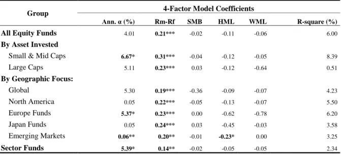
Table III. Regression Coefficients

This table presents the OLS regression coefficients for all the clusters in analysis. Ann.α is considered the clusters’ EW annualized return, in percentage, that is not explained for the model. MKT represents the exposure to the market risk and was tested to be different than 1. Coefficients for SMB, HML and WML are considered to be the exposure to the risk factors we previously explained in this thesis and were tested against zero. The 1%, 5% and 10% statistical significance levels are denoted by the symbols***,** and *, respectively.

Group 4-Factor Model Coefficients

Ann. α (%) Rm-Rf SMB HML WML R-square (%)

All Equity Funds 4.01 0.21*** -0.02 -0.11 -0.06 6.00

By Asset Invested

Small & Mid Caps 6.67* 0.31*** -0.04 -0.12 -0.05 8.39

Large Caps 5.11 0.23*** 0.03 -0.12 -0.64 0.51 By Geographic Focus: Global 5.30 0.19*** -0.36 -0.09 -0.07 4.23 North America 0.05 0.22*** -0.05 -0.13 -0.07 5.50 Europe Funds 5.37* 0.23*** 0.00 -0.62 -0.78 6.20 Japan Funds 0.05 0.24*** 0.03 -0.45 -0.03 3.58 Emerging Markets 0.06** 0.20** -0.01 -0.23* 0.00 3.25 Sector Funds 5.39* 0.14** -0.02 -0.05 -0.05 2.34

The first thing one can see in Table III is that there is only one beta coefficient for each factor in each cluster. That happens due to the fact that we regress the entire period against the factors. The only factor that is significant for all clusters is the market factor (MKT). In that sense, one may argue that returns are attributable to exposure to the market portfolio and therefore, to systematic risk. Nothing can be inferred from the others. This fact can be mainly due to two hypotheses: the first one is that, since Famma and French factors are built based on stocks’ returns, they might not be the most appropriate to explain mutual funds returns. The second one is simply arguing that there is no statistical reason to claim mutual funds returns are driven by exposure to size, growth and momentum factors. Table III also provides information on the model fitness. In this case, the explanation power of the model is very low, since the R-square of the regressions range from 0.51% to 8.39%. In that sense, both hypotheses can be seen as complementary towards each other. By analyzing the first column of the table, one can understand that only four clusters provide positive and significant alpha, which may actually mean managers of funds included in those clusters show better “stock

1

12 picking” ability than those who manage funds in other clusters. All in all, for five of our clusters, results are in accordance with Famma and French (2010), who argue that if there are funds’ managers with better “stock picking” skills, they are hidden in the group of those who do not have this type of skill. Our results do not completely support Famma and French (2010) due to the fact that we find positive and significant alphas that range from 0.06% to 6.67%. Our results do not have an implication on how easy is to find the best managers within each cluster. We just provide evidence that is not necessary to try to find them. By investing in EW indices, investors are rewarded by funds managers’ ability to pick stocks.

We find there are some clusters that tend to present better managers. However, our results are mixed, since in five clusters our results are inconclusive. These results can be attributed to several reasons. Firstly, one can argue results might have been different if we had used mutual funds’ factors, which we did not. The second reason is that, in fact, there is no “stock picking” skill in some mutual funds’ managers, or at least, there is no way to identify which managers do have that skill.

In order to study if these conclusions hold for investors, we decided to implement investment strategies in which the only criteria to invest is past performance, measured in three different ways: Raw Returns, Sharpe Ratio and Certainty Equivalent.

III. Investment Strategy

Past performance of assets has been used as main criteria of investment decisions. The belief that assets’ past returns provide information on future ones’ has led people to invest in some specific securities and pursue persistence investment strategies, especially on equities. Jegadeesh and Titman (1993) demonstrate that buying past winners and selling equities of companies that performed the worst in the past delivers positive and significant abnormal returns. Rowenhorst (1998) demonstrates that internationally diversified portfolios consisting of past winners outperform those which comprise past losers, at least in the mid-term, even after correcting performance for risk. Griffin et al. (2005) study returns persistence and conclude that price momentum strategies generate higher returns than market indices. As in the previously mentioned paper, we study the performance of persistence strategies using a sample of 20,879 equity mutual funds worldwide. Some advantages arise from the use of

13 these types of strategies in this study and the comparison of their performance with others. Firstly, simplicity of implementation may be very useful for investors since they can easily understand how to make a profit without having to spend time and money to gain additional knowledge of financial markets. Moreover, the fact that we compare the performance of strategies which only difference can be attributable to funds managers’ skills might bring additional insights about the existence of funds managers’ “stock picking ability”.

As mentioned before, we do not study momentum strategies. Whereas conventional momentum strategies imply no investment at moment zero, since one buys past winners and sells those assets that performed the worst; we only hold long positions in funds that performed the best during the estimation period. The investment strategies we use to conduct our study are based in a very simple persistence criterion: invest in the mutual funds that perform the best in the past. Therefore, we rank the funds according to their past performance. Past performance can be measured using different variables. By using raw returns and risk-adjusted performance measures in our analysis, namely Sharpe Ratio and Certainty Equivalent to sort the funds, we intend to provide deeper knowledge and intuition on persistence strategies and to take into consideration levels of risk in the funds we include in our strategies.

Since we want to evaluate the performance of the strategies over several time horizons, we use different estimation and holding periods. From now on, estimation period is defined as the number of months we use to compute the value of the variable we use to rank funds in each cluster. Holding period is the number of months an investor would hold the portfolio. Figure

I provides graphical information on how we implement our investment strategy.

Figure I shows the mechanics of our investment strategy. In the first column, one can see an

example of a sample of ten equity mutual funds of any cluster we mentioned before. During the estimation period of 𝑛 months, we compute the compounded return or Return of Estimation Period (REP), Sharpe Ratio or Certainty Equivalent of each fund. In the end of the estimation period (𝑡), we rank portfolios based on the criteria we are using at that time. We use different performance measures to rank funds during the estimation periods. However, the methodology is always the same. In that sense, we think it is unnecessary to include figures in this thesis to explain how the other strategies are implemented.

14

Figure I. Investment Strategy

In the figure, we present the mechanics of our investment strategies based on returns persistence. We use an example in which the sample comprises only ten equity mutual funds. This example is considering we rank funds based on Past Raw Returns. Since the methodology we used is the same when ranking funds based on past Sharpe Ratios or Certainty Equivalent is the same, we feel this figure is representative of all of our strategies

Investment Strategy

REP (%) Rank Invest and Hold

(𝑡 − 𝑛) 𝑡𝑜 𝑡 𝑡 (𝑡 + 1) 𝑡𝑜 (𝑡 + ℎ)

Fund I 2.35 Fund III 5.03 Fund III 5.03

Fund II -1.42 Fund X 4.04

Fund III 5.03 Fund IX 3.48

Fund IV -2.71 Fund I 2.35

Fund V -3.53 Fund VI 1.72

Fund VI 1.72 Fund VII 0.46

Fund VII 0.46 Fund VIII -0.71

Fund VIII -0.71 Fund II -1.42

Fund IX 3.48 Fund IV -2.71

Fund X 4.04 Fund V -3.53

In Figure I one can see an example in which we use Raw Returns to estimate which funds performed the best during the estimation period. The day after we invest in the funds included in the top decile. In this case, we invest our money solely in Fund III, due to the fact that it was the fund that delivered the best compounded return amongst the ten funds in the sample. Then, we hold the portfolio of funds for ℎ months, which we define as the holding period. Meanwhile, we measure the performance of funds in the sample for the next holding period. The implementation of this strategy implies that whenever the holding period is lower than the estimation period, there are some months that are included more than once in the estimation window. When holding period is bigger than the estimation period, this situation no longer occurs. As we stated before, we sort funds and build portfolios based on funds’ Raw Returns, Sharpe Ratio and Certainty Equivalent. Whereas our estimation periods are set as 3, 6, 12, 36 and 60 months when sorting based on raw returns, we only consider estimation periods of 12 months or longer when ranking funds based on the previously mentioned risk-adjusted performance measures. Regarding holding periods, we consider for all variables 1, 3, 6 and 12 months, which implies we only study short-term persistence of returns. We consider all the possible combinations of estimation and holding periods for each cluster, which results in 20 different strategies per cluster, in the case when funds are sorted according to past returns. We study 180 different short-term strategies, when the ranking variable is past returns. When we rank funds based on past Sharpe Ratio or Certainty Equivalent, we conduct

15 a study on more 216 investment strategies. All in all, we end up conducting a study about the performance of 396 different investment strategies. Performance measures as Annualized Mean Return, Standard Deviation and Sharpe Ratios are computed and presented further in this thesis. Since we use several different holding periods, it was necessary to make some adjustments to the factors, which we did by computing the compounded return of the factors for a period equal to the strategies’ estimation period.

IV. Results

As shown before, the results of our regressions are mixed. Within our clusters, there are four clusters (Emerging Markets, Sector, European and Small & Mid Caps) that present positive and significant alphas. However, for the others, we find no statistical reason to claim funds managers are better or worse than others in picking stocks. In order to better assess if investors would have any benefit in relying in funds’ managers ability to pick the better stocks amongst those existent in the financial markets, we conduct Out-of-Sample implementation of 396 different persistence investment strategies.

Table IV shows Annualized Mean Returns, Standard Deviation of returns and Annualized

Sharpe Ratios for every strategy we implemented. As mentioned before, we started by ranking funds according to their past performance, with different estimation periods. We then build portfolios of funds by buying participation units of those funds which were included in the top decile. In that sense, we end up holding Equally Weighted Indices of funds during the holding period. In the end of the holding period, we sell all the participation units and buy ones from the funds that performed the best during the estimation period. In order to take into account risk of each fund, we rank funds not only based on past returns. We apply exactly the same methodology we described before, but we buy funds who delivered investors the highest Sharpe Ratio or Certainty Equivalent. In this study, we assume Certainty Equivalent can be computed with the underlying assumption that utility follows a power-utility function with a risk-aversion coefficient (𝛾) of 2. When ranking funds according to the risk-adjusted performance measures we discussed earlier, we only consider estimation periods equal or longer than 12 months, so that we guarantee representativeness of these measures.

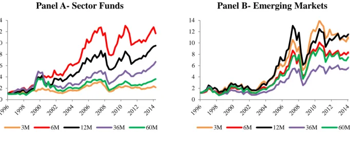
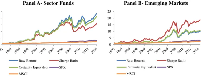
16 We think presenting results only for the entire sampling period may disregard some important features of our investment strategies, namely performance differences under different economic environments. Therefore, further in this thesis, we show the results of the additional analysis we make. We start by graphically showing performance differences for different estimation periods. We also compare the results of the same strategy with different ranking criteria. In order to properly compare our investment strategies with passively managed ones, we not only compute indices that demonstrate investors would be granted higher returns if they had invested in our strategies but we also compare risk-adjusted performance of our strategies with the performance of the previously mentioned passively managed investment strategies. Fees do also have a major role when studying whether or not investors would benefit from investing in mutual funds. In our strategies, fees are very important due to the fact that, whenever we rebalance our portfolios, we incur in extra costs. We expect investment strategies with shorter holding periods to be jeopardized the most.

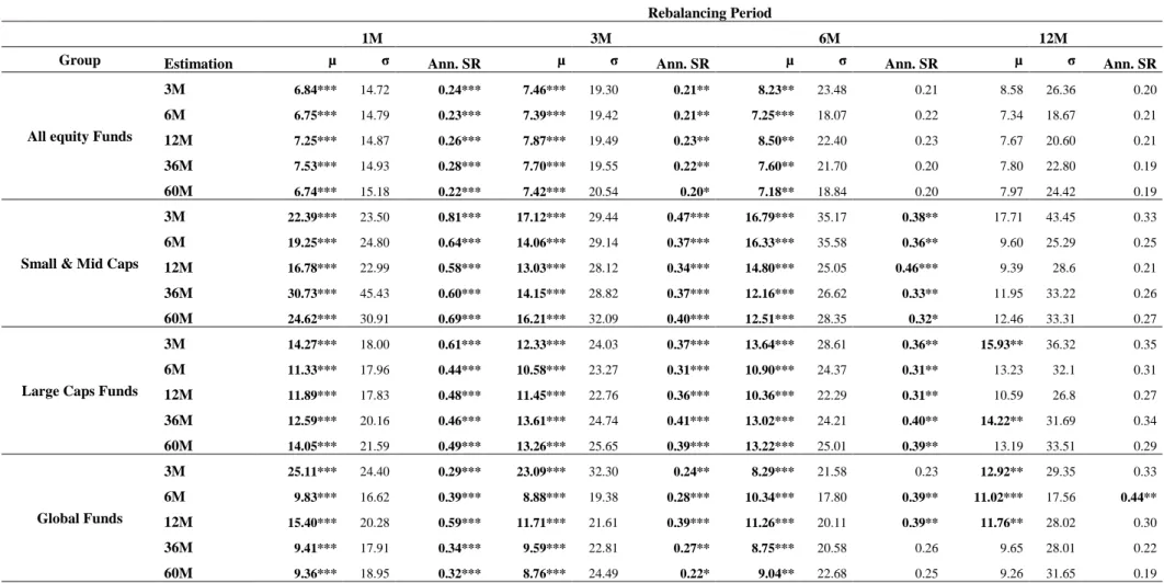
We start by presenting our strategies’ performance without taking into consideration the impact of redemption fees. Tables IV, V, and VI show the results of our strategies. We focus mainly on three annualized performance or risk measures: Returns, Sharpe Ratio and Standard Deviation of returns. One can find Annualized Mean Return of each strategy, with different estimation and holding periods. Even though return can be considered a performance measure, investors shall not forget that information on risk is not incorporated in returns. In order to better analyze performance, we use risk-adjusted performance measures, namely Sharpe Ratios that measures additional return investors would be provided for each additional unit of standard deviation they bear when investing in these momentum strategies. We use Certainty Equivalent because it takes into consideration skewness and kurtosis of returns’ distribution. Some conclusions can be drawn from analyzing Table IV. Firstly, one can see that, for rebalancing periods of 1 month, returns of all clusters are positive and significant. The same happens when the rebalancing period is half a year, excepting the Japan cluster. Furthermore, when rebalancing periods are longer, returns tend to still be positive and significant, for short estimation periods. Whereas the top three performers in very short rebalancing periods are Small & Mid Caps, Sector and Emerging Markets clusters, the worst performer is the Japan cluster, for every holding and estimation periods. When comparing performance of funds that invest in small caps with those that invest in large caps, our results are in accordance with those of Rouwenhorst (1998), which concludes small caps returns’ are more persistent than large caps’ ones.

17

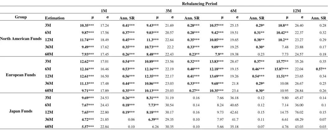
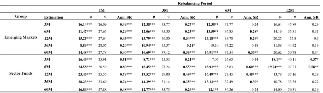
Table IV. Strategy based on Past Returns Results

Table IV presents Annualized Returns (µ), Annualized Standard Deviation and Sharpe Ratio for every strategy of each cluster we introduced earlier in this thesis. We tested significance of Annualized Mean Returns against zero. The 1%, 5% and 10% statistical significance levels are denoted by the symbols***,** and *, respectively

Rebalancing Period

1M 3M 6M 12M

Group _Estimation µ σ _{Ann. SR} µ σ _{Ann. SR} µ σ _{Ann. SR} µ σ _{Ann. SR}

All equity Funds

3M 6.84*** 14.72 0.24*** 7.46*** 19.30 0.21** 8.23** 23.48 0.21 8.58 26.36 0.20 6M 6.75*** 14.79 0.23*** 7.39*** 19.42 0.21** 7.25*** 18.07 0.22 7.34 18.67 0.21 12M 7.25*** 14.87 0.26*** 7.87*** 19.49 0.23** 8.50** 22.40 0.23 7.67 20.60 0.21 36M 7.53*** 14.93 0.28*** 7.70*** 19.55 0.22** 7.60** 21.70 0.20 7.80 22.80 0.19 60M 6.74*** 15.18 0.22*** 7.42*** 20.54 0.20* 7.18** 18.84 0.20 7.97 24.42 0.19

Small & Mid Caps

3M 22.39*** 23.50 0.81*** 17.12*** 29.44 0.47*** 16.79*** 35.17 0.38** 17.71 43.45 0.33 6M 19.25*** 24.80 0.64*** 14.06*** 29.14 0.37*** 16.33*** 35.58 0.36** 9.60 25.29 0.25 12M 16.78*** 22.99 0.58*** 13.03*** 28.12 0.34*** 14.80*** 25.05 0.46*** 9.39 28.6 0.21 36M 30.73*** 45.43 0.60*** 14.15*** 28.82 0.37*** 12.16*** 26.62 0.33** 11.95 33.22 0.26 60M 24.62*** 30.91 0.69*** 16.21*** 32.09 0.40*** 12.51*** 28.35 0.32* 12.46 33.31 0.27

Large Caps Funds

3M 14.27*** 18.00 0.61*** 12.33*** 24.03 0.37*** 13.64*** 28.61 0.36** 15.93** 36.32 0.35 6M 11.33*** 17.96 0.44*** 10.58*** 23.27 0.31*** 10.90*** 24.37 0.31** 13.23 32.1 0.31 12M 11.89*** 17.83 0.48*** 11.45*** 22.76 0.36*** 10.36*** 22.29 0.31** 10.59 26.8 0.27 36M 12.59*** 20.16 0.46*** 13.61*** 24.74 0.41*** 13.02*** 24.21 0.40** 14.22** 31.69 0.34 60M 14.05*** 21.59 0.49*** 13.26*** 25.65 0.39*** 13.22*** 25.01 0.39** 13.19 33.51 0.29 Global Funds 3M 25.11*** 24.40 0.29*** 23.09*** 32.30 0.24** 8.29*** 21.58 0.23 12.92** 29.35 0.33 6M 9.83*** 16.62 0.39*** 8.88*** 19.38 0.28*** 10.34*** 17.80 0.39** 11.02*** 17.56 0.44** 12M 15.40*** 20.28 0.59*** 11.71*** 21.61 0.39*** 11.26*** 20.11 0.39** 11.76** 28.02 0.30 36M 9.41*** 17.91 0.34*** 9.59*** 22.81 0.27** 8.75*** 20.58 0.26 9.65 28.01 0.22 60M 9.36*** 18.95 0.32*** 8.76*** 24.49 0.22* 9.04** 22.68 0.25 9.26 31.65 0.19

18

Table IV (Continued) . Strategy based on Past Returns Results

Table IV presents Annualized Returns (µ), Annualized Standard Deviation and Sharpe Ratio for every strategy of each cluster we introduced earlier in this thesis. We tested significance of Annualized Mean Returns against zero. The 1%, 5% and 10% statistical significance levels are denoted by the symbols***,** and *, respectively

Rebalancing Period

1M 3M 6M 12M

Group _Estimation µ σ _{Ann. SR} µ σ _{Ann. SR} µ σ _{Ann. SR} µ σ _{Ann. SR}

North American Funds

3M 10.35*** 17.24 0.41*** 9.43*** 21.69 0.28*** 10.57*** 25.15 0.29* 10.8** 26.40 0.28 6M 9.87*** 17.56 0.37*** 9.03*** 20.57 0.28*** 9.42*** 19.51 0.31** 10.42** 22.37 0.32 12M 11.74*** 18.49 0.45*** 11.3*** 22.64 0.35*** 10.85*** 19.65 0.38** 10.2** 23.27 0.29 36M 9.49*** 17.62 0.35*** 10.73*** 22.2 0.33*** 9.09*** 19.25 0.30* 7.48 23.88 0.17 60M 7.93*** 17.45 0.26*** 8.48*** 22.43 0.23** 7.9** 19.38 0.23 7.73 24.57 0.18 European Funds 3M 12.62*** 17.01 0.54*** 10.89*** 23.56 0.32*** 13.83*** 28.47 0.37** 15.77** 35.26 0.35 6M 12.16*** 16.46 0.53*** 12.16*** 22.19 0.40*** 12.18*** 19.15 0.46*** 15.87*** 22.04 0.57** 12M 12.61*** 16.50 0.56*** 12.35*** 22.17 0.41*** 13.69*** 19.26 0.54*** 11.51** 23.65 0.34 36M 11.13*** 17.48 0.44*** 10.86*** 23.03 0.33*** 9.68*** 21.8 0.29* 10.08 26.67 0.25 60M 9.71*** 17.89 0.35*** 10.13*** 25.03 0.27** 10.35*** 23.4 0.30* 10.95 28.84 0.26 Japan Funds 3M 9.69*** 24.53 0.26*** 8.31*** 31.19 0.16 7.66 36.18 0.12 9.80 45.47 0.14 6M 7.67*** 24.43 0.18*** 7.73** 30.54 0.14 8.24 40.65 0.12 7.14 36.00 0.1 12M 7.65*** 22.80 0.19*** 8.18*** 30.17 0.16 9.73 42.61 0.15 14.75 76.02 0.15 36M 4.72*** 21.85 0.06 6.39** 29.35 0.10 7.97 41.7 0.11 6.61 48.29 0.07 60M 5.57*** 22.84 0.10 6.26 30.35 0.10 5.66 35.18 0.07 4.76 43.03 0.03

19

Table IV (Continued) . Strategy based on Past Returns Results

Table IV presents Annualized Returns (µ), Annualized Standard Deviation and Sharpe Ratio for every strategy of each cluster we introduced earlier in this thesis. We tested significance of Annualized Mean Returns against zero. The 1%, 5% and 10% statistical significance levels are denoted by the symbols***,** and *, respectively

Rebalancing Period

1M 3M 6M 12M

Group _Estimation µ σ _{Ann. SR} µ σ _{Ann. SR} µ σ _{Ann. SR} µ σ _{Ann. SR}

Emerging Markets 3M 16.14*** 26.09 0.49*** 12.38*** 33.77 0.27** 12.38** 37.77 0.24 16.64 45.89 0.29 6M 11.47*** 27.65 0.29*** 12.06*** 35.30 0.25** 13.59** 36.85 0.28* 14.16 35.31 0.31 12M 15.25*** 27.64 0.43*** 15.79*** 36.80 0.34*** 13.18*** 33.78 0.29* 20.25 55.8 0.3 36M 8.89*** 28.05 0.20*** 10.94*** 35.37 0.21* 10.10 37.22 0.18 11.88 44.32 0.19 60M 14.48*** 27.78 0.40*** 16.69*** 37.12 0.36*** 16.91*** 37.54 0.36** 20.62 50.78 0.34 Sector Funds 3M 16.46*** 25.91 0.51*** 8.71*** 25.53 0.21** 7.06 26.63 0.14 18.1** 40.11 0.37* 6M 24.58*** 26.59 0.80*** 18.45*** 27.24 0.55*** 18.92*** 25.83 0.60*** 19.24*** 27.23 0.58** 12M 23.46*** 25.55 0.79*** 17.52*** 29.00 0.49*** 16.49*** 27.45 0.48*** 13.78 37.16 0.28 36M 28.23*** 33.69 0.74*** 14.39*** 31.14 0.35*** 13.12*** 32.49 0.30* 10.78 33.35 0.22 60M 16.86*** 27.88 0.48*** 12.77*** 35.75 0.26** 12.1** 36.26 0.24 14.00 56.31 0.19

20

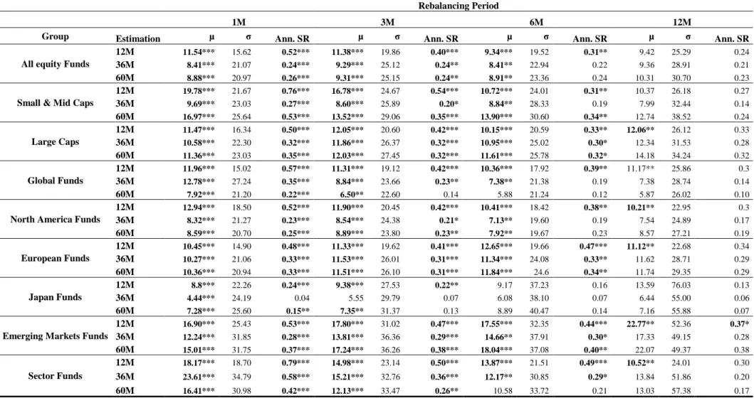
Table V. Strategy based on Sharpe Ratio Results

Table V presents Annualized Returns (µ), Annualized Standard Deviation and Sharpe Ratio for every strategy of each cluster we introduced earlier in this thesis. We tested significance of Annualized Mean Returns against zero. The 1%, 5% and 10% statistical significance levels are denoted by the symbols***,** and *, respectively.

Rebalancing Period

1M 3M 6M 12M

Group _Estimation µ σ _{Ann. SR} µ σ _{Ann. SR} µ σ _{Ann. SR} µ σ _{Ann. SR}

All equity Funds

12M 11.54*** 15.62 0.52*** 11.38*** 19.86 0.40*** 9.34*** 19.52 0.31** 9.42 25.29 0.24 36M 8.41*** 21.07 0.24*** 9.29*** 25.12 0.24** 8.41** 22.94 0.22 9.36 28.91 0.21 60M 8.88*** 20.97 0.26*** 9.31*** 25.15 0.24** 8.91** 23.36 0.24 10.31 30.70 0.23 Small & Mid Caps

12M 19.78*** 21.67 0.76*** 16.78*** 24.67 0.54*** 10.72*** 24.01 0.31** 10.37 26.18 0.27 36M 9.69*** 23.03 0.27*** 8.60*** 25.89 0.20* 8.84** 28.33 0.19 7.99 32.44 0.14 60M 16.97*** 25.64 0.53*** 13.52*** 29.06 0.35*** 13.90*** 30.60 0.34** 12.74 38.52 0.24 Large Caps 12M 11.47*** 16.34 0.50*** 12.05*** 20.60 0.42*** 10.15*** 20.59 0.33** 12.06** 26.12 0.33 36M 10.58*** 22.30 0.32*** 11.86*** 26.37 0.32*** 10.95*** 25.02 0.30* 12.34 31.53 0.28 60M 11.36*** 23.03 0.35*** 12.03*** 27.45 0.32*** 11.61*** 25.78 0.32* 14.18 34.24 0.32 Global Funds 12M 11.96*** 15.02 0.57*** 11.31*** 19.12 0.42*** 10.36*** 17.92 0.39** 11.17** 25.86 0.3 36M 12.78*** 27.24 0.35*** 8.84*** 23.66 0.23** 7.38** 21.38 0.19 7.38 28.74 0.14 60M 7.92*** 21.20 0.22*** 6.50** 22.60 0.14 5.88 21.24 0.12 5.87 26.02 0.10 North America Funds

12M 12.94*** 18.50 0.52*** 11.90*** 20.45 0.42*** 10.41*** 18.42 0.38** 10.21** 22.95 0.3 36M 8.32*** 21.27 0.23*** 8.54*** 24.38 0.21* 7.13** 19.60 0.19 7.54 24.89 0.17 60M 8.59*** 20.70 0.25*** 8.89*** 23.80 0.23** 7.92** 19.67 0.23 8.57 27.21 0.19 European Funds 12M 10.45*** 14.90 0.48*** 11.33*** 19.62 0.41*** 12.65*** 19.66 0.47*** 11.12** 22.68 0.34 36M 10.27*** 21.06 0.33*** 11.53*** 26.01 0.31*** 11.34*** 24.08 0.33** 11.62 28.71 0.29 60M 10.36*** 20.94 0.33*** 11.51*** 26.10 0.31*** 11.84*** 24.6 0.34** 11.74 29.35 0.29 Japan Funds 12M 8.8*** 22.26 0.24*** 9.38*** 27.53 0.22** 9.17 37.23 0.16 13.59 76.03 0.13 36M 4.44*** 24.19 0.04 5.55 29.79 0.07 6.08 38.10 0.07 6.44 55.00 0.06 60M 7.28*** 25.60 0.15** 7.35** 31.37 0.13 8.89 40.47 0.14 7.16 55.88 0.07 Emerging Markets Funds

12M 16.90*** 25.43 0.53*** 17.80*** 31.02 0.47*** 17.55*** 32.35 0.44*** 22.77** 52.36 0.37* 36M 12.24*** 31.85 0.28*** 13.81*** 36.36 0.29*** 14.66** 37.91 0.30* 17.33 49.15 0.28 60M 15.01*** 31.75 0.37*** 17.24*** 36.26 0.38*** 18.04*** 37.08 0.40** 22.07 49.37 0.38 Sector Funds 12M 18.17*** 18.70 0.79*** 14.98*** 23.14 0.50*** 13.87*** 21.51 0.49*** 10.52** 24.01 0.30 36M 23.61*** 34.79 0.58*** 15.21*** 32.76 0.36*** 12.17** 30.85 0.29* 13.84 51.86 0.20 60M 16.41*** 30.98 0.42*** 12.13*** 33.47 0.26** 10.58 33.72 0.21 13.03 57.38 0.17

21

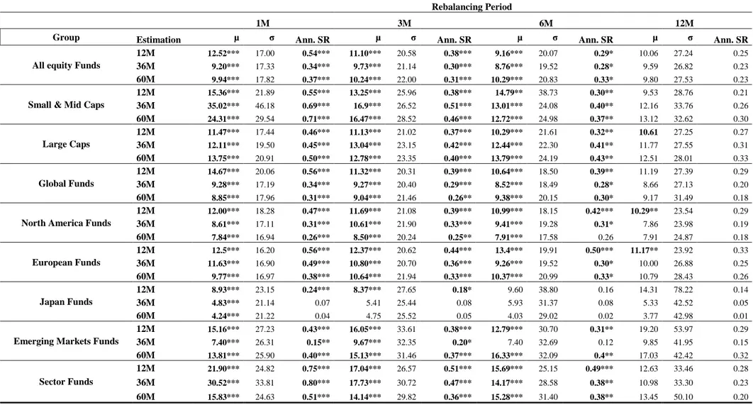
Table VI. Strategy based on Certainty Equivalent Results

Table VI presents Annualized Returns (µ), Annualized Standard Deviation and Sharpe Ratio for every strategy of each cluster we introduced earlier in this thesis. We tested significance of Annualized Mean Returns against zero. The 1%, 5% and 10% statistical significance levels are denoted by the symbols***,** and *, respectively.

Rebalancing Period

1M 3M 6M 12M

Group _Estimation µ σ _{Ann. SR} µ σ _{Ann. SR} µ σ _{Ann. SR} µ σ _{Ann. SR}

All equity Funds

12M 12.52*** 17.00 0.54*** 11.10*** 20.58 0.38*** 9.16*** 20.07 0.29* 10.06 27.24 0.25 36M 9.20*** 17.33 0.34*** 9.73*** 21.14 0.30*** 8.76*** 19.52 0.28* 9.59 26.82 0.23 60M 9.94*** 17.82 0.37*** 10.24*** 22.00 0.31*** 10.29*** 20.83 0.33* 9.80 27.53 0.23 Small & Mid Caps

12M 15.36*** 21.89 0.55*** 13.25*** 25.96 0.38*** 14.79** 38.73 0.30** 9.53 28.76 0.21 36M 35.02*** 46.18 0.69*** 16.9*** 26.52 0.51*** 13.01*** 24.08 0.40** 12.16 33.76 0.26 60M 24.31*** 29.54 0.71*** 16.47*** 28.52 0.46*** 12.72*** 24.98 0.37** 13.12 32.62 0.30 Large Caps 12M 11.47*** 17.44 0.46*** 11.13*** 21.02 0.37*** 10.29*** 21.61 0.32** 10.61 27.25 0.27 36M 12.11*** 19.50 0.45*** 13.04*** 23.15 0.42*** 12.44*** 22.30 0.41** 11.77 27.55 0.31 60M 13.75*** 20.91 0.50*** 12.78*** 23.35 0.40*** 13.79*** 24.19 0.43** 12.51 28.01 0.33 Global Funds 12M 14.67*** 20.06 0.56*** 11.32*** 20.31 0.39*** 10.64*** 18.50 0.39** 11.19 27.39 0.29 36M 9.28*** 17.19 0.34*** 9.27*** 20.40 0.29*** 8.52*** 18.49 0.28* 8.66 27.13 0.20 60M 8.85*** 17.96 0.31*** 9.04*** 21.46 0.26** 9.38*** 20.15 0.30* 9.17 31.49 0.18 North America Funds

12M 12.00*** 18.28 0.47*** 11.69*** 21.08 0.39*** 10.99*** 18.15 0.42*** 10.29** 23.54 0.29 36M 8.61*** 17.11 0.31*** 10.61*** 21.90 0.33*** 9.41*** 19.28 0.31* 7.86 23.98 0.19 60M 7.84*** 16.94 0.26*** 8.50*** 20.24 0.25** 7.91*** 17.58 0.26 7.91 24.87 0.18 European Funds 12M 12.5*** 16.20 0.56*** 12.37*** 20.62 0.44*** 13.4*** 19.91 0.50*** 11.17** 23.92 0.33 36M 11.63*** 16.90 0.49*** 10.80*** 20.70 0.36*** 9.26*** 19.52 0.30* 10.00 26.88 0.25 60M 9.77*** 16.97 0.38*** 10.64*** 21.94 0.33*** 10.37*** 20.99 0.33* 10.79 28.43 0.26 Japan Funds 12M 8.93*** 23.15 0.24*** 8.37*** 27.65 0.18* 9.60 38.80 0.16 14.31 78.22 0.14 36M 4.83*** 21.14 0.07 5.41 25.44 0.08 5.93 31.37 0.08 5.33 42.52 0.05 60M 4.24*** 21.22 0.04 4.75 25.52 0.05 4.03 29.02 0.02 3.77 42.98 0.01 Emerging Markets Funds

12M 15.16*** 27.23 0.43*** 16.05*** 33.61 0.38*** 12.79*** 30.70 0.31** 19.20 53.97 0.29 36M 7.40*** 26.31 0.15** 9.67*** 32.35 0.20* 7.40 32.69 0.12 9.85 41.95 0.15 60M 13.81*** 25.90 0.40*** 15.13*** 31.46 0.37*** 16.33*** 32.09 0.4** 17.03 42.42 0.32 Sector Funds 12M 21.90*** 24.82 0.75*** 17.04*** 26.57 0.51*** 15.69*** 25.15 0.49*** 12.63 33.46 0.28 36M 30.52*** 33.81 0.80*** 17.73*** 30.72 0.47*** 14.17*** 28.58 0.38** 10.98 33.30 0.23 60M 15.83*** 24.63 0.51*** 14.14*** 29.82 0.36*** 15.28*** 31.40 0.38** 13.45 50.10 0.20

22 We also reach the same conclusions as Griffin et al (2005), who finds profitable for investors to invest in American stocks with the best past performance. One should also take into account that investing in mutual funds do carry high levels of risk. Annualized Standard Deviation of returns varies from a minimum of 17.0% to a maximum of almost 44.0 In terms of risk-adjusted performance; we find that almost every strategy rewards investors with positive and significant Sharpe Ratios. We are also able to claim the shortest the rebalancing period, the higher the Shape Ratio tends to be. If they investors had invested in strategies as ours, they would be granted Sharpe Ratios up to 0.81.

In Table V, we present the results of our portfolios, which were built based on funds’ past Sharpe Ratios. In this case, our shortest estimation period is 12 months. We only use estimation periods of one year and longer for more accurate estimation of funds’ Sharpe Ratios. The first conclusion one may draw form observing Table V is that, for rebalancing periods lower than 6 months, every return is positive and almost everyone is significant at the one percent level. Moreover, returns tend to be high, as is evidence the Annualized Returns of 18.17% investors would be granted if they had invested their money in the Sector Funds’ cluster. Returns of 19.78% or 16.90% would also be possible if one had allocated part of their portfolio to momentum strategies which invest in the Small & Mid Cap or Emerging Markets’ clusters. On the other hand, buying funds that invest in Japanese equities would give investors very low returns at a very high risk. The Annualized Mean Returns in the Japanese cluster are the lowest amongst our clusters, which is mainly due to the two crises Japan went through during the sampling period. Another conclusion that one can take by analyzing the same table is that this type of strategies are very risky, as can be inferred by the Annualized Standard Deviation of almost 35% in the Sector Fund cluster. However, these strategies provide positive Annualized Sharpe Ratios that can go up to a maximum of 0.79, which is almost three times as the one investors could achieve by investing in the Standard & Poor’s 500 Index. In that sense, there is some room to argue some of our strategies do have better risk-adjusted performance than some passive strategies. We also claim that 30% of our strategies based on past Sharpe Ratios deliver an Annualized Sharpe Ratio of, at least, 0.3, which corresponds approximately to the historical S&P500 Sharpe Ratio. When analyzing Table V, one can also conclude that there most of clusters’ returns are always significant for part of the rebalancing periods. As examples, one can see that when the estimation period is 12 months, returns of portfolios of funds which invest in Emerging Markets are positive and significant up to 12 months of rebalancing period. Exceptions are the All Equity Funds, Small & Mid