CMOS Design and Implementation of a
Reduced-KII Multiplexed Network
Rui Graça
Mestrado Integrado em Engenharia Eletrotécnica e de Computadores Supervisor: Professor Cândido Duarte
Co-Supervisor: Professor Vítor Grade Tavares
The need for massively parallel computing strategies has increased over the last years, chiefly due to the increasing demand for real-time pattern recognition applications. Nature and several million years of evolution have provided human beings with a highly-parallel and fault tolerant mecha-nism for solving such problems - the brain. Hence, it is of practical interest to artificially mimic brain operation with the clear objective of embedding evermore "intelligence" into engineering applications. This idea is not new, and the concept of artificial neural networks is well established in the scientific community and more recently in industry. It should be noticed however that the relationship between most artificial neural networks and accurate physiological models is a rather loose bond.
Analog VLSI is a promising technology for implementing these massively parallel algorithms, favouring solutions with low-power and area consumption. However, massively parallel systems are generally massively interconnected, which poses big challenges for VLSI design.
In this work, the RKII network, a biologically realistic model of the olfactory bulb is studied and implemented in analog VLSI. Although it is intrinsically very different from generic feed-forward or recursive artificial neural networks, the basic processing cells are very similar in both cases, and as with the last, interconnections are an important issue.
The RKII network is a set of coupled oscillators, and it behaves as a content addressable mem-ory, much like a Hopfield network. However, differently than the Hopfield network, trajectories in space state are limit cycles. This dynamic behavior allows quick state transition upon input change.
Early implementations of the model decreased the burden of interconnections by time multi-plexing the system. These implementations served as a proof of concept. In this work, a system implementation based on earlier approaches, but with capacity for small practical applications, is studied and designed.
A necessidade de formas de computação altamente paralelas tem vindo a crescer nos últimos anos, principalmente devido ao aumento da importância de aplicações de reconhecimento de padrões em tempo real. A natureza, juntamente com milhões de anos de evolução, forneceu ao ser humano um mecanismo de computação altamente paralelo e tolerante a falhas - o cérebro. A mimetização artificial do nosso cérebro é, portanto, uma boa base de partida para o desenvolvimento de apli-cações dotadas de inteligência, com interesse em apliapli-cações de engenharia. Esta ideia não é nova, e o conceito de rede neuronal artificial está bem estabelecido na comunidade científica e, mais recentemente, na indústria. É importante referir, no entanto, que a relação entre a generalidade das redes neuronais artificiais e modelos fisiológicos mais precisos é bastante vaga.
VLSI analógico é uma tecnologia com elevado potencial para a implementação destes algo-ritmos altamente paralelos, com baixo consumo de potência e com baixa ocupação de área. No entanto, sistemas altamente paralelos são geralmente altamente interligados, o que impõe grandes desafios em implementações VLSI.
Neste trabalho, a rede RKII, um modelo biologicamente realista do bolbo olfativo é estudado e implementado em VLSI analógico. Apesar de ser intrínsecamente diferente das redes neuronais artificiais, as células elementares de processamento são semelhantes em ambos os casos, e, tal como nas redes neuronais artificiais, a implementação das interconexões é uma questão importante a resolver.
A rede RKII é um conjunto de osciladores acoplados, que se comporta como uma memória endereçável por conteúdo, à semelhança da rede de Hopfield. No entanto, ao contrário do que acontece na rede de Hopfield, as trajetórias no espaço de estados são oscilatórias. Este comporta-mento dinâmico permite uma mudança rápida do estado perante a mudança da entrada.
Implementações anteriores do mesmo modelo usaram multiplexagem temporal para diminuir o número de interconexões físicas. Estas implementações foram usadas como prova de conceito. Neste trabalho, é estudada e proposta uma implementação de um sistema baseado nas abordagens anteriores, mas com capacidade para pequenas aplicações práticas.
I would like to thank my supervisors, Professor Cândido Duarte and Professor Vítor Tavares, for all the guidance and the support in this work. Moreover, I thank them for proposing me such an interesting work to develop and explore.
I thank Microelectronics Students’ Group for all technical support, without which, this work would not be possible.
I thank my family, specially my parents and my brother, for all the moral support and for being always available to help me with everything.
I thank my friends for the encouragement and for the interest shown towards this work. I specially thank Rita for the emotional support and for being always on my side.
Rui Graça
1 Introduction 1
1.1 Modeling the Brain . . . 2
1.2 Artificial Neural Networks . . . 3
1.3 Freeman Olfactory Neural System model . . . 5
1.4 Objectives and Approach . . . 6
1.5 Structure of the Document . . . 7
2 Background and Related Work 9 2.1 The Perceptron and Feedforward Neural Networks . . . 9
2.2 Recurrent Neural Networks and Hopfield Networks . . . 12
2.3 VLSI Implementations of Neural Networks . . . 13
2.4 Freeman Olfactory Neural System model . . . 15
3 System Modeling and Architecture 23 3.1 Filter and Hold . . . 23
3.2 The Multiplexed RKII Network . . . 26
3.2.1 RKII Set Simulation . . . 29
3.2.2 RKII Network Simulation . . . 33
3.3 BIST . . . 37
3.3.1 BIST Algorithm Simulation . . . 38
3.4 Network implementation . . . 38
3.4.1 Pins . . . 42
3.4.2 Memories . . . 43
3.4.3 Registers . . . 43
3.4.4 Control structure and system architecture . . . 44
3.4.5 Time operation . . . 46
4 Multiplexed RKII Network Design 49 4.1 Filter Design . . . 49
4.1.1 Transconductance Amplifier Design . . . 50
4.1.2 Filter Integration . . . 53
4.2 Memory Design . . . 57
4.3 Sigmoid Design . . . 60
4.4 RKII network integration . . . 61
4.4.1 Sigmoid and Memory integration . . . 61
4.4.2 Memory and weight capacitors integration . . . 62
4.4.3 RKII network integration . . . 62
4.5 Improvements to the network implementation . . . 65 vii
4.6 Control Structure . . . 71
4.6.1 Control Structure Operation . . . 73
5 BIST Design and System Integration 77 5.1 BIST Design . . . 77
5.1.1 Checker Circuit Algorithm . . . 77
5.1.2 Amplifier Block Design . . . 81
5.1.3 Comparator Block Design . . . 83
5.1.4 Checker Circuit Integration . . . 84
5.1.5 Peak Detector Block Design . . . 85
5.1.6 Peak Detector Amplifier Design . . . 87
5.1.7 Peak Detector Integration . . . 87
5.1.8 BIST Control Structure . . . 87
5.2 System Integration . . . 89
6 Conclusions and Future Work 93 6.1 Future work . . . 94
A Layout Plots 95 A.1 RKII Network . . . 95
A.1.1 Transconductance amplifier . . . 95
A.1.2 Filter . . . 96
A.1.3 Delay block . . . 96
A.1.4 RKII set . . . 97
A.1.5 RKII network with three sets . . . 97
A.1.6 Excitatory sigmoid . . . 98
A.1.7 Inhibitory sigmoid . . . 99
A.2 BIST . . . 100
A.2.1 Amplifier . . . 100
A.2.2 Comparator . . . 101
A.2.3 Checker circuit . . . 102
A.2.4 Peak Detector amplifier . . . 103
A.2.5 Peak Detector . . . 104
1.1 Interface between the brain and the outside world. . . 2
1.2 Artificial neuron. . . 3
1.3 Feedforward neural network with one hidden layer. . . 4
1.4 The KII and the RKII. . . 6
2.1 Linearly separable and non-linearly separable problems. . . 10
2.2 XOR mapped to a two layer network. . . 11
2.3 Logistic function. . . 12
2.4 Hopfield network with three nodes. . . 13
2.5 Cellular Neural Network. . . 14
2.6 The KO. . . 15
2.7 Nonlinearity in the KO . . . 16
2.8 KII network. . . 17
2.9 The KIII. . . 18
2.10 RKII network. . . 19
3.1 Multiplexed RKII network. . . 24
3.2 Simple Filter and Hold RC circuit. . . 24
3.3 Single pole Filter and Hold model simulation. . . 25
3.4 Switched Gm-C filter schematics. . . 26
3.5 Two pole Filter and Hold model simulation. . . 27
3.6 Two pole Filter and Hold Cadence Virtuoso simulation. . . 27
3.7 Filter and Hold frequency analysis and comparison with continuous time filter. . 28
3.8 Continuous and multiplexed RKII set response to a square wave. . . 30
3.9 Influence of the interconnection weights on the RKII operation. . . 31
3.10 Changes in dynamics due to decrease in sampling frequency. . . 32
3.11 Discrete time RKII set. . . 33
3.12 Comparison between discrete time model in Virtuoso and difference equations. . 34
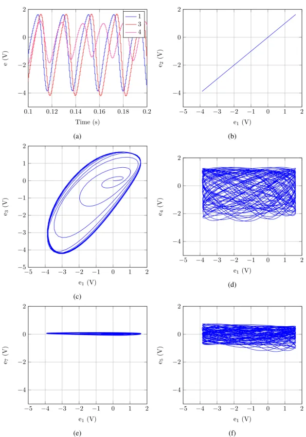
3.13 Excitatory states of an RKII network with 16 sets. . . 35
3.14 Simulation results of an RKII network with 16 sets. . . 36
3.15 BIST model simulation. . . 39
3.16 Multiplexed network implementation. . . 40
3.17 Global and distributed control structure in the RKII network. . . 41
3.18 Toplevel block diagram of the system. . . 46
3.19 Control signals for the time operation of the multiplexed network. . . 47
4.1 Transconductance amplifier topology. . . 50
4.2 Transconductance amplifier static test. . . 51
4.3 Transconductance amplifier static test results. . . 52 ix
4.4 Post-layout filter simulatios. . . 54
4.5 Filter offset analysis. . . 56
4.6 Delay block schematics. . . 57
4.7 Sigmoid block. . . 59
4.8 Post-layout sigmoid characteristic. . . 59
4.9 Memory and weight capacitor integration. . . 63
4.10 RKII network post-layout simulation. . . 64
4.11 Influence of interconnection capacitance in post-layout simulation. . . 66
4.12 Post layoyt simulation of an RKII network with 16 sets. . . 67
4.13 Post layout simulation results of an RKII network with 16 sets. . . 68
4.14 Integrator configuration. . . 69
4.15 Interconnection voltage versus sigmoid output using the integrator in Figure 4.14. 70 4.16 Multiplexed transconductance amplifiers. . . 70
4.17 Multiplexed filter. . . 71
4.18 RKII network with multiplexed filter simulations. . . 72
4.19 Control structure time diagram. . . 74
5.1 Original checker circuit used in the BIST. . . 79
5.2 Checker circuit proposed. . . 80
5.3 Amplifier block schematics. . . 81
5.4 Amplifier simulations. . . 82
5.5 Comparator block schematics . . . 83
5.6 Comparator block simulations. . . 84
5.7 Checker circuit with regenerator . . . 85
5.8 Checker algorithm simulations. . . 86
5.9 Peak detector block . . . 86
5.10 Operational amplifier used in peak detector . . . 87
3.1 Control signals in the multiplexed network. . . 40
3.2 List of pins in the final system implementation. . . 43
3.3 Blocks in the global control structure. . . 44
3.4 Blocks in the local control structures. . . 45
4.1 Transconductance amplifier transistor dimensions. . . 51
4.2 Transconductance amplifier Monte Carlo static analysis. . . 52
4.3 Capacitance values used in filters. . . 53
4.4 Delay block transistor dimensions. . . 58
4.5 Delay block simulation results. . . 58
4.6 Delay block Monte Carlo analysis. . . 58
4.7 Sigmoid block transistor dimensions. . . 58
4.8 Excitatory sigmoid block Monte Carlo analysis. . . 61
4.9 Inhibitory sigmoid block Monte Carlo analysis. . . 61
4.10 Sigmoid block settling time. . . 61
4.11 Cascaded sigmoid and delay block settling time. . . 62
4.12 Control structure synthesis results. . . 72
5.1 Checker circuit control signals. . . 78
5.2 Amplifier transistor dimensions. . . 82
5.3 Comparator transistor dimensions . . . 83
5.4 Comparator inverter transistor dimensions . . . 84
5.5 Peak Detector amplifier transistor dimensions . . . 87
5.6 Area occupation and current consumption of analog blocks. . . 89
ASIC application-specific integrated circuit BIST built-in self test
CAM content-addressable memory CNN cellular neural network CS chip select
EEG electroencephalogram F&H filter and hold
FPGA field-programmable gate array GPU graphics processing unit LMS least-mean-square MLP multilayer perceptron SCL serial clock
SDI serial data in SDO serial data out
SPI serial peripheral interface VLSI very-large-scale integration XOR exclusive OR
Introduction
Over the years, the traditional digital computer has proven to be an extremely powerful tool, performing many tasks much better and faster than humans. Operations such as the multiplication of large numbers, which take a considerable amount of time for a human being to complete, are performed in a few nanoseconds by digital computers. However, there are still operations in which our brain performs much better than any computer. It is able to learn from experience, and based on that, it is able to recognize data in extremely noisy environments. For instance, it is extremely easy for humans to identify a familiar face and to associate that face to a certain person in completely different situations. Even if the face is partially covered, seen from different angles or even if it has changed considerably, we are able to associate it to the right person. This kind of operations are extremely difficult to implement with intrinsically sequential algorithms on traditional computers. However, they are quite interesting from an engineering point of view. Pattern recognition and machine learning are fields that are becoming more and more important, since more efficient ways to learn from data, and to abstractly recognize data in noisy environment are demanded. Among important applications that would benefit from more efficient pattern recognition, we can highlight computer-aided medical diagnosis, the recognition of handwritten characters and speech recognition. All these tasks are relatively simple to humans, therefore research about computation in the brain offers engineers a starting point for the development of electronic machines based on how the brain operates, which may be able to solve problems as humans do.
Although appealing, the implementation of electronic devices based on biological evidence is not a simple task. The brain is massively interconnected, and interconnections are a huge problem in very-large-scale integration (VLSI) implementations. Hence, direct application of most models for computing machines are not scalable. In this work, an approach based on time multiplexing is followed [1]. This approach significantly reduces the burden of the interconnections at the cost of a more complex digital control structure.
Outside World
Brain
Receptors Effectors
Figure 1.1: Interface between the brain and the outside world.
1.1
Modeling the Brain
It is reasonable to consider that modeling the brain is fundamental for conceiving engineering systems with similar functionalities. In fact, as stated by Haykin [2], “the brain is the living proof that fault tolerant parallel computing is not only physically possible, but also fast and powerful”. It is the central element of the nervous system and it is constituted by nervous cells, commonly known as neurons.
As depicted in Figure 1.1, the brain receives information from the outside world (or from within the body) through receptors and acts on the outside world through effectors. Both receptors and effectors are essential to the operation of the brain, since they provide the interface between physical external information and signals that can be processed by the brain. These signals, known as action potentials or spikes, are voltage pulses. Spikes propagate within a neuron through its axon, a relatively long line, which can be modelled as an RC transmission line [2]. Neurons communicate with each other by synapses, being the chemical synapse the most common interface. In a chemical synapse, the occurrence of patterns of action potentials causes the release of a chemical substance, the neurotransmitter, from the pre-synaptic neuron. This substance is received by a post-synaptic neuron, triggering a pattern of action potentials [3]. This kind of synapse is an electrical to chemical conversion followed by the reverse conversion. A synapse can either have excitatory or inhibitory effects over the post-synaptic neuron.
Although early studies tried to model the brain similarly to a digital computer [4], there are evidences that behavior and precise functions result from the organization of neural circuits, mak-ing the paradigm of the logical computer unsuitable for modelmak-ing the brain [3, 5, 6]. This gave rise to a new paradigm, known as connectionism [5], that defends that the way neurons are connected with each other is determinant to their function. In this way, networks of neurons are formed with information stored in the interconnections.
Based on the same principles as connectionists, and due to the large density of interconnec-tion among neurons, another paradigm appeared, suggesting that neural activity is best explained observing masses of neurons, or neural sets. Under such assumption, the brain is considered a continuum and is modeled by continuous differential equations [6–8], whereas in the study of in-dividual neurons, action potentials are used as the observable basis of study. Conversely, the study
x2 w2
Σ
f yx1 w1
..
.
..
.
xn wn
Figure 1.2: Artificial neuron.
of neural masses is based on the observation of electroencephalogram (EEG) waveforms [6]. Early studies suggested that the brain cortex had distinct functional regions [9], meaning that language was treated by a section of the brain, movement by a distinct section, smell by some other section, and so on. According to theory of mass action [10], however, this is not entirely true. In his work, Lashsley observed that the capability of a rat with a brain lesion to learn a task is much more dependant on the severity of the lesion than on its exact location. He concluded that the brain is highly redundant, since, under deprivation of a sensory capability, a function that would usually be associated to the region of the lesion can still be performed using some other region of the cortex.
The study of computation in the brain, commonly known as computational neuroscience [11], aims to model and to understand the mechanisms used by the brain to execute functions. The brain is generally modeled as a nonlinear dynamical system [12].
Concluding, the brain can be viewed as a massively parallel computer. It is highly redundant and, therefore, highly fault tolerant. Its operation, however, is radically different than the one of a digital computer.
1.2
Artificial Neural Networks
An artificial neural network is the earliest engineering system inspired on (loose) biological evi-dence. It consist of several nodes, known as artificial neurons, which perform parallel computation. A typical artificial neuron is depicted in Figure 1.2.
The concept appeared in the 1940s, with the first mathematical model of a neural network, proposed by McCulloch and Pitts [4]. After that, the field of neural networks became quite active. The goal was both to understand how the brain works at a level higher than synapses and action potentials, and to develop a machine able to perform the same kind of tasks that the brain is good at, exploring highly parallel computation approaches. A major step in the development of neural networks was the perceptron [5]. The perceptron is a single-layer feedforward neural network. This means that, besides the input layer, which receives the input signals from the outside (and does not perform any computation), there is only one other layer of neurons, known as the output
Input layer Hidden layer Output layer
...
...
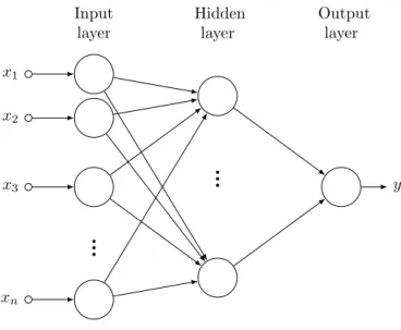
x1 x2 x3 xn yFigure 1.3: Feedforward neural network with one hidden layer.
layer. The function of a perceptron is controlled by properly adjusting the interconnection between the input and the output layers. Since it is feedforward, there are no connections neither between nodes in the same stage nor from the output stage to the input stage. As demonstrated later, the perceptron is very limited, in the way that many useful functions cannot be mapped, being the exclusive OR (XOR) a typical example of a function not mappable in the perceptron [13]. This fact significantly reduced the interest in artificial neural networks.
Later developments in the field introduced the concepts of hidden layers and recurrent net-works, that significantly extend the range of problems solvable by neural netnet-works, in relation to the perceptron. Hidden layers are layers between the input and the output stage of the network. Again, in feedforward networks, there are only connections between neurons from a layer to the following one. In this way, hidden layers do not receive inputs from the outside and their output is not an output of the network, therefore the name ‘hidden’. A simple neural network with one hidden layer may be found in Figure 1.3.
The inclusion of feedback loops in neural networks may bring interesting properties. Networks with feedback are usually known as recurrent neural networks. In such networks, the output of a stage may be the input of a previous stage. Recurrent neural networks may or may not have hidden layers. A common example of a recurrent network is the Hopfield network [14]. Hopfield networks are used as content-addressable memories (CAMs) (or associative memories) in which a learned pattern affected by noise at the input can be recovered at the output.
As referred before, the behavior of a neural network is controlled by the interconnection weights. The process of adjusting the weights to obtain a desired response is known as learning. The learning process may be either supervised or unsupervised, and may be either deterministic or stochastic.
In its genesis, artificial neural networks aimed to model the brain, in order to study how it operates at the level of learning and behavior. However, developments in this field significantly diverged from this goal, and generally, there are few similarities between artificial neural net-works and more accurate models of the brain. However, there is still interest in the development of realistic electronic systems that mimic the brain operation. This field, known as neuromor-phic engineering, is a highly multidisciplinary field, since it requires knowledge of neurosciences, electronic engineering and nonlinear dynamical systems.
Because neurons comprise a summation block, a nonlinear function, and interconnections that are weighted replicas of the output from other cells, and since they are intrinsically parallel, neural networks are clearly suited for an analog VLSI implementation. However, there are also digital implementations proposed in the literature, either using field-programmable gate arrays (FPGAs) or implemented on application-specific integrated circuits (ASICs). As already referred, both cases are subject to a big problem common to many other electronic applications - the interconnectivity. Biological neural networks are highly interconnected, and so are most artificial neural network models. In a totally connected feedforward network, the number of connections increases with the square of length of the input vector [15]. This is clearly unscalable, therefore, other approaches must be followed in order to overcome this problem.
1.3
Freeman Olfactory Neural System model
In contrast with many earlier approaches, Walter J. Freeman modelled the olfactory neural system not from the neuron level, but from a mesoscopic approach, based on the observation of EEG waveforms [6]. The model is defined hierarchically, with each level denoted by K, after Katchal-sky, for his earlier work. The most basic cell is the KO, which includes a summation block, a linear second order low-pass filter and a sigmoid. A KI is formed by connecting two KO acting over each other with either positive weight (excitatory pair) or negative weight (inhibitory pair). The KII is composed by four KO. As shown in Figure 1.4a, two of the KO have positive (excitatory) outgoing weights, and the other two have negative (inhibitory) outgoing weights. By properly adjusting the weights, a KII behaves as an oscillator controlled by the input, in which a positive input causes the output to oscillate, and an input of 0 causes the output to vanish to 0. A KII network is formed by several KII interconnected. The highest level of the model is the KIII, and it is composed by blocks of lower levels.
The Reduced KII (RKII), shown in Figure 1.4b is a simpler cell, consisting only of two KO (one excitatory and one inhibitory), but has a behavior similar to the one of KII [6]. It is signifi-cantly simpler to use in practical applications than the KII, since it has fewer KO cells and fewer connections, which means that it has fewer parameters to adjust, and therefore it is simpler to study and train.
The KII network, and consequently also the RKII network, models the olfactory bulb, which plays a fundamental role in the identification of odorant stimuli [16]. Both the KII and the RKII networks behave as CAMs, much like Hopfield networks [17, 18]. However, differently than
Input K0E,1 K0E,2 K0I,2 K0I,1 + + + − + − − + − − (a) Input K0E K0I Kie + Kei − (b)
Figure 1.4: a) KII and b) RKII.
Hopfield networks, equilibrium points in the state space are unstable, resulting in oscillatory tra-jectories. Moreover, the KIII has chaotic basal dynamics. Both these characteristics result in that it requires less energy to change from one equilibrium point to another [16].
1.4
Objectives and Approach
In this work, a CMOS implementation of an RKII network is proposed. In order to mitigate the large number of interconnections, time multiplexing is used [1], so that the number of physical interconnections scales linearly with the number of cells, keeping the same number of logical interconnections. Moreover, time multiplexing enables the possibility of resource sharing, which, besides reducing the area and power consumption, mitigates possible problems due to mismatches. The cost of the multiplexed approach is that it requires digital control in order to properly select the active cell at the right time.
In order to further reduce mismatches, a built-in self test (BIST) circuit is implemented. This circuit, proposed by Duarte et al. [19], tests cells and searches for the group of cells that have the better match with each other and selects that group of cells to be active.
Departing from small networks with few cells already implemented in previous works [1, 18, 20–25], in this work a system with enough cells for small practical applications is proposed. Moreover, a control structure for the network and for the BIST is implemented. The result is a system implementation that will enable research about the application of RKII networks in pattern classification problems.
The implementation proposed uses a 0.35 µm CMOS technology with dual power supply of ±1.65 V. The implementation is limited by area, up to a maximum of 5 mm2.
1.5
Structure of the Document
After this brief introduction, in which some basic concepts and topics that serve as motivation for this work were presented, a deeper analysis of neural networks and their implementation is pre-sented in Chapter 2, as well as a more detailed overview of Freeman’s model and its application in pattern classification. In Chapter 3, the implementation proposed in this work is further explained and modelled, and the system architecture is presented. In Chapter 4, the design of the multiplexed network is explored, as well as its control structure. In Chapter 5 the BIST design is presented, as well as some considerations about the system implementation. At last, conclusions, and future work are presented in Chapter 6.
Background and Related Work
In this chapter, the fundamentals of neural networks are explained and topics about possible hard-ware implementations are discussed. Although the origins of Freeman model are intrinsically different from typical neural networks, they have many similar applications and characteristics: the basic processing element (KO in Freeman model, neuron in artificial neural networks) are very similar. The interconnection problem is also a common issue to both the Freeman model and arti-ficial neural networks. Therefore, it is interesting to study artiarti-ficial neural networks and how the problems arising from hardware implementations were covered. Moreover, Freeman Olfactory System model is explained with more detail, focusing on aspects related with its application to pattern classification and with its implementation in hardware.
Section 2.1 focuses on the Perceptron and multilayer perceptron (MLP), Section 2.2 focuses on recursive neural networks and Section 2.3 on hardware implementation of artificial neural net-works. In Section 2.4, Freeman model is presented in detail.
2.1
The Perceptron and Feedforward Neural Networks
The perceptron was an important step in the early developments of neural networks. It consists of a single layer network, without any kind of feedback. With the perceptron, Rosenblatt aimed to create a model for computation in the brain, following a connectionist approach. This approach substantially differs from earlier ones, that were significantly influenced by developments in digital computers and symbolic logic, in the way that it aimed to mimic the behavior of the brain at a lower level [5].
The perceptron is basically a linear combiner and a threshold function, which means that its inputs are weighted and summed, and the output of the perceptron is either high (+1) or low (-1) depending on the result of the weighted sum. Hence, the perceptron classifies inputs in one of two classes. A network may be formed using several perceptrons in parallel, each one trained independently for a given function.
In order to adapt the perceptron to a desired response to a set of stimuli, a learning rule is required. The perceptron learning rule is simply an adaptive filter that drives the interconnection
x1 x2 Class 1 Class 2 (a) (1,1) (0,1) (1,0) (0,0) x1 x2 Class 1 Class 2 Class 2 (b)
Figure 2.1: a) shows a linearly separable problem, thus solvable by the perceptron, and b) shows a non-linearly separable problem (the XOR), not solvable by the perceptron.
weights to a set that ensures the desired response. This is done by setting the weights (and the threshold) to arbitrary small values. Being wn the set of weights at iteration n, yn the set of perceptron outputs for a training set x as input, using wnas weight set, d the desired set of output for x and µ the step of the algorithm, w is updated by:
wn+1= wn+ µ· (d − y) (2.1)
This rule is guaranteed to converge if the problem in question is mappable to the perceptron. Otherwise, there is no set of weights that suits the problem. The threshold value can be adjusted by this algorithm by including an extra value in the weight set, with a corresponding value of 1 in x. However, as observed by Minsky and Papert [13], the set of problems mappable to the perceptron is quite limited. In order for a problem to be solvable by the perceptron, the two output classes must be linearly separable, which means that, in the input space, there must be a linear hyperplane that divides the space in two sections, with every input that maps to the same output lying in the same section, as in Figure 2.1a. As we can see in Figure 2.1b, the XOR is an example of a non-linearly separable problem. There is no such straight line that divides the space in the desired classes. This observation significantly reduced the interest, not only in the perceptron, but in neural networks in general.
Contrary to what Minsky and Papert [13] expected, however, multilayer neural networks may be constructed to map a much wider diversity of problems. For instance, a two layer network, as seen in Figure 2.2, may be used to map the XOR [2].
An example of a generic feedforward multilayer network was already showed in Figure 1.3. In a general case, it is composed by several layers, with every cell in each layer connected to every cell in the following layer and not directly connected to any other cell. Layers other than
x1 x2 1 1 1 y 1 1 1 1 -2 1 -1.5 -0.5 -0.5
Figure 2.2: XOR mapped to a two layer network.
the input or output ones are known as hidden layers. Such networks are also known as MLPs [2]. Differently than the perceptron, MLPs usually use a sigmoid as the activation function and not a simple threshold. These functions are differentiable everywhere. A common example of a sigmoid function is the logistic function, defined by (2.2).
f(x) = 1
1+ e−x (2.2)
A plot of the logistic function may be found in Figure 2.3.
The most common learning algorithm for MLPs is back-propagation, popularized by Rumel-hart and McClelland in 1986 [26]. This algorithm is a generalization of the least-mean-square (LMS), which is also a popular algorithm for the perceptron [2]. It is an iterative algorithm, di-vided in two steps. In the first step, the response of the network for the actual set of weights is computed. In the second step, an adaptive filter is applied in order do minimize the error between the resultant response and the desired one. This is done by first computing the error for neurons in the output layer, and then iterating layer by layer, from the output to the input layer. This order is required, because the computation of the influence of a neuron to the error requires the computa-tion of the error in subsequent layers. Due to the popularity of the algorithm, MLPs are frequently referred as back-propagation networks.
More recently, more efficient learning algorithms have been developed. This, along with the advance in computational power of general purpose computers and graphics processing units (GPUs), enabled networks with many hidden layers to be feasible [27–29]. Networks with several hidden layers are generally called Deep Neural Networks and they are now a preferred technology in pattern recognition [29].
-0.2 0 0.2 0.4 0.6 0.8 1 1.2 -10 -5 0 5 10
Figure 2.3: Logistic function.
2.2
Recurrent Neural Networks and Hopfield Networks
In the previous section, the networks referred were purely feedforward. From a biological perspec-tive, this is clearly not the case in real neural networks [6], and from an engineering perspecperspec-tive, interesting applications may be achieved by the use of feedback. Neural networks that exhibit feedback are known as recurrent networks. The analysis of recurrent networks is substantially different from the one of feedforward networks, due to their inherent dynamical behaviour. The framework of nonlinear dynamical systems is, therefore, widely used for the analysis of recurrent networks.
As nonlinear systems, recurrent networks may exhibit many attractors in their state space. Computational properties of these networks are achieved by proper placement of their attractors, and learning consists in obtaining the desired placement [2].
The most common example of a recurrent neural network is the Hopfield model [14], popular-ized by Hopfield in 1982. The structure of an Hopfield network is depicted in Figure 2.4. Every neuron is connected to all other ones, but not to itself. It means that there is no self-feedback. An Hopfield network can either be discrete or continuous in time. Whereas the discrete time model uses a McCulloch-Pitts neuron, described before [14], neurons in the continuous model exhibit a low-pass linear dynamic response, cascaded with a sigmoid nonlinearity [30]. Attractors in a Hopfield network are fixed-points, meaning that it is globally stable (after a finite time, the system will converge to an equilibrium point).
It is quite intuitive that such system can be used as a CAM. A learned pattern should be stored as a state in the network state space. When a noisy and incomplete version of a stored pattern is
x
1y
1x
2y
2x
3y
3Figure 2.4: Hopfield network with three nodes.
presented at the input, the system state will converge to the stored pattern [14]. Learning consists, therefore, in properly selecting the interconnection weights so to force the desired patterns to be attractors in the state space.
As well as feedforward networks, recurrent networks may exhibit hidden layers. Examples of models of neural networks with hidden layers are the Elman networks [31] and Jordan net-works [32].
2.3
VLSI Implementations of Neural Networks
Many results about neural networks were obtained by simulations in digital computers. However, in order to fully explore their parallelism, hardware implementations are desired.
Most neural networks models have an intrinsic analog behavior. Therefore, analog VLSI im-plementations can be achieved by direct application of those models. However, due to the large number of interconnections, such implementations would not likely be scalable. In order to obtain a scalable neural network, different approaches can be followed. An option is to design digital networks. In such networks, the burden of the interconnections can be reduced by the usage of time multiplexing and resource sharing, but they are not as efficient as their analog counterpart when it comes to the accumulation of the inputs and the multiplication by the weights [15]. Ana-log implementations are more efficient in terms of area and power, but are are much more sensitive to variations in the manufacturing process [33].
The usage of hybrid networks, such as the one proposed in this work, combines advantages from both analog and digital implementations. For instance, in the multiplexed RKII network [1], digital control is used to time-multiplex an analog network, thus allowing resource sharing. This
C1,1 C1,2 C1,3 C1,4
C2,1 C2,2 C2,3 C2,4
C3,1 C3,2 C3,3 C3,4
C4,1 C4,2 C4,3 C4,4
Figure 2.5: Cellular Neural Network.
allows to reduce the number of physical interconnections without affecting the number of network-level interconnections.
Other approach to reduce the burden of the interconnections is to reduce the number of in-terconnections in the network, and not only at the physical level. This approach is followed in cellular neural networks (CNNs) [34] [35]. Such network are inspired in cellular automata. Cells are disposed in a lattice and are connected only to their physically nearest neighbours, thus reduc-ing the number of connections. Original CNNs were purely analog circuits. A CNN is depicted in Figure 2.5.
A comprehensive survey about hardware implementation of neural networks was presented by Misra and Saha [33]. All networks referred are radically different from Freeman’s model, but their implementations face similar issues.
Despite its potential, analog hardware implementation of neural networks is still an highly unexplored field. Digital implementations are much more common nowadays. An example that has recently attracted some interest is the SpiNNaker [36], which is a massively parallel spiking neural network. It was created with the to enable real-time simulation of realistic spiking neural networks for neuroscience research. It decreases the burden of interconnection by using a central node for communication. Every node is physically connected only to the central node, and not to every node in the network. The network operation is event-oriented, and nodes communicate events via addressed packets.
x2
Σ
F (s)
2ndorder dynamicsQ(x)
Assimetric sigmoid y x1..
.
xnFigure 2.6: The KO.
2.4
Freeman Olfactory Neural System model
Freeman model for the neural olfactory system was introduced by Walter J. Freeman [6]. It has been developed and applied for several engineering purposes by Freeman and many other re-searchers.
Freeman approaches the brain at a level higher than single neurons and action potentials. This level of approach is called mesoscopic [37]. At this level, the brain is modeled using differential equations, recurring to the observation of EEG waveforms as the observable basis of study. Al-though accepting the role of neurons as the fundamental cells in computation in the brain, Freeman states that, due to the interrelation of many neurons in information transmission, the observation of single or few neurons is not an efficient way to explain the inherent cooperative behavior observed in neural activity. On the other hand, the observation of neural masses, treated as a continuum and not as individual cells, is much more insightful about this cooperative behavior [6].
The most basic building block of the model is the KO set, which models a set of neurons ranging from 103to 108with common input, common sign output, and no functional interconnec-tions among them [6]. The KO, depicted in Figure 2.6, is similar to the cells in a continuous and deterministic Hopfield network [30]. It exhibits a summation node, a linear low-pass filter and a sigmoid nonlinearity. However, differently from the Hopfield network, the low-pass filter has a second order response, and the nonlinearity is an asymmetric sigmoid. The linear dynamics are given by (2.3), where a and b are the poles of the dynamic response. From biological evidence, a=220 rad/s and b =720 rad/s [6].
H(s) = a· b
(s + a)(s + b) (2.3)
The asymmetric sigmoid is depicted in Figure 2.7 and given by (2.4). Qm is the asymptotic maximum of the sigmoid function, which is found by biological evidence and it is different from layer to layer. In Figure 2.7, Qm= 5 is used, which is commonly used for the olfactory bulb [38– 41]. Q(x) = ( Qm· (1 − e−(e x−1)/Q m) , if x > ln(1− Q m· ln(1 +Q1 m)) −1 , if x< ln(1− Qm· ln(1 +Q1 m)) (2.4)
-2 -1 0 1 2 3 4 5 6 -10 -5 0 5 10
Figure 2.7: Nonlinearity in KO with Qm= 5.
The output of the linear dynamics in the KO is generally known as the KO state.
Several KO interconnected with common sign feedback form a KI set. A KI set can be either excitatory or inhibitory, depending of the sign of the connection weights. In such network, each KO is connected to every other in the network and there is no self-feedback.
A KII set is as depicted in Figure 1.4a. It consists of an excitatory KI and an inhibitory KI with dense interconnection [6]. When isolated, it behaves as an oscillator controlled by the input: an input of zero results in a zero output, and a positive input results in an oscillatory response. Several KII connected form a KII network, as depicted in Figure 2.8. In such network, inputs are applied in a excitatory KO of each KII, and there are connections both among excitatory KO of each KII and among inhibitory KO.
The higher layer of the model is named KIII. This structure, depicted in Figure 2.9 [22], contains several lower lever structures and models the entire olfactory neural system.
The KII can be simplified to a cell with only two KO. This cell is the reduced KII (RKII). As well as the KII, the RKII is an oscillator controlled by the input, and both cells result in similar responses at system level [6, 21]. An RKII network is formed in a similar way as the KII network, as can be seen in Figure 2.10. The RKII is significantly simpler to use than the KII, since it has less connections and, therefore, less weights to adjust.
KIII simulations have shown that its behavior successfully mimics EEG waveforms and its statistical properties. EEG and KIII waveforms are similar both when an odorant stimuli is given and in the absence of stimulation. Moreover, with parameter variation, the KIII can be adjusted to mimic both the waveforms obtained during epileptic seizures and during deep anesthesia [39].
x1 K0E,1 K0E,2 K0I,2 K0I,1 + + + − + − − + − − x2 K0E,1 K0E,2 K0I,2 K0I,1 + + + − + − − + − − xn K0E,1 K0E,2 K0I,2 K0I,1 + + + − + − − + − − xn−1 K0E,1 K0E,2 K0I,2 K0I,1 + + + − + − − + − − − − − − − − Kii + + + + + + Kee
Figure 2.8: KII network.
on feedback loops. Evidence suggest that the KIII has the capacity to learn input patterns by adjusting the weights of excitatory to excitatory connections in the KII network that models the olfactory bulb [40, 42]. Every other interconnection weight is fixed. A learned pattern results in the formation of an attractor in the KIII state space. In this way, when a learned pattern is presented at the input, the KIII state converges to a near-limit cycle (low-dimension chaotic wing) that internally represents the input pattern [16,40]. After learning, a landscape of low-dimensional chaotic local basins of attraction is formed, with each basin corresponding to a learned pattern [43]. Moreover, the system has the capacity to successfully recognize a learned pattern if it is distorted or incomplete [42]. This properties are the ones of a CAM.
In the absence of an input, both the KIII and biological evidence have a high-dimensional chaotical behavior [39]. This basal chaotic state enables fast convergence to every learned state when an input is presented. When an unknown pattern is presented, a characteristic chaotic be-havior arises, which suggests that the chaotic bebe-havior of the KIII has an important role in learn-ing [16,39,40]. These characteristics are considerably different from the ones found in common re-cursive neural networks such as the Hopfield model, where chaos is treated as undesirable [14,30]. In the KIII, chaos is not only an intrinsic characteristic, but it brings properties that are interesting for pattern classification, since it enables fast and ready state transition when the input changes.
Due to these interesting properties, the KIII has been tested for pattern classification applica-tion. Learning is done by adjusting excitatory to excitatory weights in the olfactory bulb, gener-ally in a Hebbian way. Hebbian learning is a common learning rule, in which a synaptic weight is strengthened when the respective two neurons are activated by the same input [2]. The first learning rule proposed for the KIII was a modified Hebbian rule [17]. It is a binary rule - it sets a interconnection weight to a fixed high value if two inputs are active in any input pattern in the learning set and to a low value otherwise. Although quite simple and limited in the number of patterns than can be stored simultaneously, this rule has shown good results [17, 42]. A simple modification to this rule uses three weights instead of two [44]. If two KII are active
simulta-x1 x2 xn−1 xn Input fromreceptors
K0E + K0E K0E + K0E
+
+ + +
Periglomerular Layer (KI net-work) K0E,1 K0E,2 K0I,2 K0I,1 + + + − + − − + − − K0E,1 K0E,2 K0I,2 K0I,1 + + + − + − − + − − K0E,1 K0E,2 K0I,2 K0I,1 + + + − + − − + − − K0E,1 K0E,2 K0I,2 K0I,1 + + + − + − − + − − − − − − − − Kii + + + + + + Kee
Σ From all K0E,1
Olfactory Bulb Layer (KII net-work) K0E,1 K0E,2 K0I,2 K0I,1 + + + − + − − + − − Anterior Olfactory
Nucleus Layer (KII set) K0E,1 K0E,2 K0I,2 K0I,1 + + + − + − − + − − Prepyriform Cortex
Layer (KII set)
K0E,1 − + External Capsule Layer (K0 set) f1 f2 f3 f4 Σ To all K0I,1 To all K0E Dispersive Delays
x1 K0E K0I Kie + Kei − x2 K0E K0I Kie + Kei − xn−1 K0E K0I Kie + Kei − xn K0E K0I Kie + Kei − − − − − − − Kii + + + + + + Kee
Figure 2.10: RKII network.
neously for only one input in the learning set, the weight between them is set to a high value, if they are never simultaneously active for any input they are set to a low value, and if they are simultaneously active for more than one input pattern, the weight is set to an intermediate value.
More recently, learning has been done by three processes simultaneously [43]: Hebbian, habit-uation and normalization. The Hebbian process may be either the binary process referred above, or a reinforcement process, in which the weights between two KII are linearly increased they are active for the same input pattern [45]. Habituation is the gradual decrease of the weights if they are not reinforced by Hebbian learning, and normalization is used to maintain stability.
Using these processes, the KIII has shown good performance in several pattern recognition applications. It has been used successfully for character classification [41, 45, 46], face recogni-tion [47], and for classificarecogni-tion of odorants [48, 49]. Moreover, it has shown positive results in time series prediction [50, 51].
An extension to the KIII model was proposed by Kozma et al. [52–54]. It includes an higher level in the hierarchy, the KIV, which models higher cognitive processes and intentionality. It is constituted by three interacting KIII. One KIII models sensory cortical functions, other KIII models the hippocampus, which is responsible for spatial and temporal orientation, and the other KIII models the midline forebrain, which is responsible for internal sensory functions. It has been used successfully as artificial brain of goal-oriented autonomous agents [52, 53, 55].
A major problem in the Freeman model is that, due to its nonlinear, and even chaotic, dynamic behavior, a mathematical analysis of its learning properties is far from straightforward. Although there already interesting results [17, 24, 40, 43, 45, 56–58], the dynamical analysis of a KIII or even a KII network is still an unsolved problem in many ways.
At the RKII set level, interesting results may be found by bifurcation analysis of an RKII set [59]. This analysis shows that, under the right choice of weights, the RKII is an oscillator
controlled by the input. It has a single attractor, and, depending on the weights and the value of the input, the attractor can be either a point or a limit cycle. Naming m∗1and g∗1 the state of the excitatory and inhibitory KO, respectively, the bifurcation occurs for [59] (Kei is the inhibitory to excitatory connection weight, and Kie the excitatory to inhibitory weight, as depicted in Fig-ure 2.10): |Kie· Kei| = 1 Q0(m∗1)· Q0(g∗ 1) ·(a + b) 2 a· b (2.5)
If|Kie·Kei| is lower than this value, the attractor is stable, if its higher, the attractor is unstable. A stable attractor corresponds to convergent equilibrium point, and an unstable attractor corre-sponds to oscillation. For an input of 0, both m∗1and g∗1are 0, and Q0(m∗1)· Q0(m∗1) = 1, therefore, the bifurcation point is simply [59]:
|Kie· Kei| =
(a + b)2
a· b (2.6)
However, for inputs different than zero, the assessment must be done case by case. Based on this expressions, three different cases can be obtained by properly selecting the weights. If |Kie· Kei| is less than the bifurcation point for both zero and the value of the high input, there RKII will be always stable (there will be no oscillation). If it is lower than the bifurcation point for zero input but higher for the high input, the RKII will oscillate when the input is high, but oscillations will fade for an input of zero. At last, if|Kie· Kei| is higher than the bifurcation point for both zero and high input, it will oscillate for both cases. In this last case, however, oscillations will have different characteristics (such as phase and amplitude) in both cases. Although the Freeman model is based on operation when the attractor is stable for low input and oscillatory for high input, applications with oscillatory attractors for both cases also exhibit computational properties [60].
As seen in Figure 2.9, the olfactory bulb is modeled by a KII network. Its approximation by an RKII network is reasonable and often used [6, 21]. The olfactory bulb plays an important role in odorant discrimination and in learning [16, 61]. KII and RKII networks alone may also be used as CAMs [24, 42, 44, 62], but with a significantly worse performance than the KIII [42].
Results presented for KIII performance in practical applications were obtained by computer simulations. Due to the system complexity, these simulations are highly computer intensive, mak-ing the simulation time quite long [45]. For this reason, real-time hardware implementations are demanded for more powerful applications. However, as in the general case for neural networks, the number of interconnections imposes a big problem in practical realizations of the Freeman model.
The first hardware implementation reported was a microprocessor-based RKII network with eight RKII sets [18]. The burden of interconnection was reduced by sampling and multiplexing the several RKII sets in the network.
Model discretization along with time multiplexing became the most common strategy used. It was used in the first analog VLSI implementation of a KII set [20], and later for the first analog VLSI implementation of an RKII network [21], constituted by four RKII sets. Relatively to the
previous implementation, besides the size reduction, these implementations introduced the usage of filter and hold (F&H), which enables the large time constants intrinsic to the model to be practi-cally achievable in VLSI. Later, this implementation was improved by sharing the sigmoid blocks among RKII sets [23], which decreases mismatches. This strategy was used to build a network with eight RKII sets [24].
In a radically different strategy, a modification was proposed to the model [25]. It replaced the sigmoid non-linearity by a integrate-and-fire block, transforming the KO in a spiking neuron. While this is not consistent with the biological origins of the Freeman model, the modified model dynamics are similar to the original one. Following this strategy, a single RKII set was tested on chip [25].
These implementations confirm that a discrete time VLSI implementation allows a real-time application of the Freeman model. However, in order to allow real-time usability for practical applications, an algorithm that uses the multiplexed RKII network in a KIII must be implemented, and an RKII network with enough RKII sets for practical application must be achieved.
System Modeling and Architecture
The approach followed in this work is based on the strategy proposed by Tavares et al. [1], which decreases the burden of the interconnections between cells by the usage of time-multiplexing. Figure 3.1 shows the multiplexing architecture [19], which allows the sigmoid blocks to be shared by all the cells, hence mitigating problems due to mismatch that would likely occur if one block per cell was used. An important difference between the original and the multiplexed network model is that the latter operates in discrete time. Therefore, filters are also discrete time, and a delay was introduced in the feedback loop.
The price to pay for the multiplexed network is the need for a digital control structure, in order to properly activate the cells in their time slots. Multiplexing also enables the usage of F&H [63]. This technique consists in switching the filter on and off with a certain duty cycle, increasing the time constant of the filter by the inverse of the duty cycle. Therefore, large time constants are achieved with not prohibitively large resistors and capacitors, and with a low power consumption. In order to further improve matching between cells, a BIST scheme [19] is also employed. This scheme selects the set of cells with the best matching (even if their parameters are not the closest to the designed ones) and selects that set to be active. Cells that significantly differ from this set are disabled. The BIST implements an offset test that checks if there are cells with significant offset, and a dynamic test that selects cells that have the closest oscillation amplitude in response to a sinusoidal input.
In this chapter, the proposed system architecture is presented. Firstly, the F&H technique is explained and modeled in Section 3.1. The operation of the multiplexed network is explained in Section 3.2. The BIST algorithm is presented in Section 3.3 and the final system architecture and the control structure are described in Section 3.4.
3.1
Filter and Hold
As stated in literature [6], the linear dynamics of the KO consists of a low pass filter with real valued poles at 220 rad/s and 720 rad/s. A realization of a filter with such low-frequency poles using common discrete time techniques such as switched-capacitor or switched-current is neither
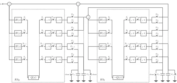
in + H(z) S1 z−1 2 S1 z−1 2 trupd Gie G1 H(z) S1 z−1 2 S1 z−1 2 trupd Gei Gii H(z) S2 z−1 2 S2 z−1 2 trupd Gie G2 H(z) S2 z−1 2 S2 z−1 2 trupd Gei Gii H(z) Sn−1 z−1 2 Sn−1 z−1 2 trupd Gie Gn−1 H(z) Sn−1 z−1 2 Sn−1 z−1 2 trupd Gei Gii H(z) Sn z−1 2 Sn z−1 2 trupd Gie Gn H(z) Sn z−1 2 Sn z−1 2 trupd Gei Gii Q(x) Cee
clean Cie clean +
−Q(x)
Cii
clean Cei clean +
K0E K0I
Figure 3.1: Multiplexed RKII network.
area nor power effective [64]. Filter and hold [63, 64] is a technique that consists of switching a filter with a time constant RC with a duty cycle α, as depicted in Figure 3.2. If the switch control signal Φ has a duty cycle of α, the time constant of the switched filter is multiplied by α1.
Assuming an input vin sampled with period T and a filter control signal Φ with period T and duty cycle α, if the switch is closed at time nT , the voltage initially stored at the capacitor will be the one stored at the end of the previous clock round, vout[n− 1]. If the switch is kept closed for infinite time, the voltage stored at the capacitor converges to the current value of vin, vin[n− 1]. Hence, the value of vout up from the moment the switch is closed follows (3.1).
vout(t) = vin[n− 1] + (vout[n− 1] − vin[n− 1])e−
t
RC (3.1)
If the switch is opened at time α and remains closed until the end of the clock cycle, the voltage voutat time T will be the same as at time αT , resulting in (3.2) [63].
vout[n] = vout(T ) = vout(αT ) = vin[n− 1] + (vout[n− 1] − vin[n− 1])e−
aT
RC (3.2)
R Φ
C
vin vout
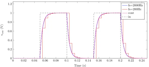
0 0.02 0.04 0.06 0.08 0.1 0.12 0.14 0.16 0.18 0.2 0.22 0.24 0 0.2 0.4 0.6 0.8 1 1.2 Time (s) vout (V) fs=2000Hz fs=200Hz cont in
Figure 3.3: Single pole Filter and Hold model simulation.
The transfer function for the filter is, therefore, given by (3.3) [63].
H(z) = (1− e− aT RC)· z−1 1− e−aTRC· z−1
(3.3) As desired, the time constant is increased by a factor of 1a, thus by scaling R· C, high time constants are achievable from smaller values of R and/or C.
Figure 3.3 shows the output of an ideal F&H block, simulated in Matlab using (3.2), with aT
RC=220 rad/s. As seen in the figure, the output of the filter is equal to a sampled version of the output of a continuous time RC filter with the time constant scaled by α1.
Another property of the F&H, also made evident by (3.3), is that the pole and zero positions relative to the input bandwidth is independent of the sampling frequency. As long as the filter duty cycle is kept constant, adjusting the sampling frequency affects time resolution but not the relative pole and zero positions [64].
The filter in the RKII has two real valued poles, one at 220 rad/s and one at 720 rad/s. In this work, the filter is implemented using a switched Gm-C filter, depicted in Figure 3.4 [63]. The transconductance amplifiers shown are equal and their transconductance is Gm. The difference equation for such filter was derived and is presented in (3.4). vmis the voltage stored by C1, τ1is the time constant of the first stage C1
Gm (not considering the F&H scaling factor), and, equivalently, τ2is GC2m. a and b are, respectively, e
−α T
τ1 and e− α T
τ2. Again, α is the F&H duty cycle and T is the sampling period. vm[n] = vin[n− 1] · (1 − a) + vm[n− 1] · a vout[n] = vin[n− 1] ·τ 1 1−τ2 · (τ1· (1 − a) − τ2· (1 − b)) +vout[n− 1] · b +vm[n− 1] ·ττ1 1−τ2 · (a − b) (3.4)
− + Φ C1 − + Φ C2 vin vout
Figure 3.4: Switched Gm-C filter schematics.
The response for a filter with original poles at 220 krad/s and 720 krad/s and scaled by α = 0.001 are shown in Figure 3.5 and compared with a continuous time response of a filter with poles at 220 rad/s and 720 rad/s. As we can see, the same properties observed in the single pole case are held, and both time constants are scaled by a factor of α1.
A filter with the same parameters as above was modelled in Cadence Virtuoso R with ideal elements and compared with a continuous time RC filter, also modelled in Virtuoso with ideal elements. Figure 3.6 shows the response of both filters to a square wave.
The only difference to the results obtained with the difference equation model is that the output changes from vout[n−1] to vout[n] at time (n−1)T +α, because the filter is active at the beginning of the clock period. Therefore, the output changes its value from t= (n− 1)T to t = (n − 1)T + α and holds this value until t= nT . Therefore, at t = nT , the value of the output vout[n] is still equal to the output of the continuous time filter. This occurs independently of the phase of the filter control signal.
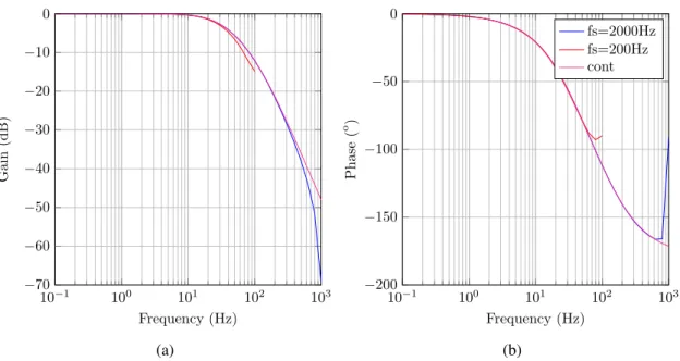
The frequency response of F&H filters with the same poles and duty cycle as the cases above, and with sampling frequencies of 200 Hz and 2000 Hz were obtained in Virtuoso using a Spectr-eRF Periodic AC analysis and the result is shown in Figure 3.7. The figure also shows the fre-quency response of a continuous time filter with poles at 220 rad/s and 720 rad/s. F&H achieves an identical frequency response as the continuous time case up to near half the sampling frequency.
3.2
The Multiplexed RKII Network
The structure of the multiplexed network is presented in Figure 3.1. Each row inside dashed rect-angles corresponds to a KO, being that the dashed rectangle on the left corresponds to excitatory KO cells, and the rectangle on the left corresponds to inhibitory KO cells. The switches at the end of each row together with the capacitors shared by all rows establish the interconnections. The output of the z−12 memories is a current signal, and the interconnection weight is controlled by the fraction of time that the corresponding switch is conducting, according to (3.5), where C is the interconnection capacitance and ∆t is the amount of time that is used for charging the capacitor in
0 0.02 0.04 0.06 0.08 0.1 0.12 0.14 0.16 0.18 0.2 0.22 0.24 0 0.2 0.4 0.6 0.8 1 1.2 Time (s) vout (V) fs=1000Hz fs=200Hz cont in
Figure 3.5: Two pole Filter and Hold model simulation.
0 0.02 0.04 0.06 0.08 0.1 0.12 0.14 0.16 0.18 0.2 0.22 0.24 0 0.2 0.4 0.6 0.8 1 1.2 Time (s) vout (V) fs=200Hz cont in
10−1 100 101 102 103 −70 −60 −50 −40 −30 −20 −10 0 Frequency (Hz) Gain (dB) (a) 10−1 100 101 102 103 −200 −150 −100 −50 0 Frequency (Hz) Phase ( o ) fs=2000Hz fs=200Hz cont (b)
Figure 3.7: Filter and Hold frequency analysis and comparison with continuous time filter (a) magnitude resuponse, (b) phase response.
each slot.
K=∆t
C [V/A] (3.5)
Each KO cell is controlled by a signal Si. Time multiplexing is achieved by activating the Si signals sequentially and separately for each i. A RKII is formed by two KO (one inhibitory and one excitatory) controlled by the same Si signal. Moreover, the filter for each KO is also activated when the respective Sisignal is active, so that the input of the KO is sampled at the right time. The signal trupd ensures simultaneous update of the outputs of all cells. This is required for coherent operation of the network, since it ensures that in every round, every cell is using the output computed in previous round for every interconnection.
In the original algorithm [19], the interconnections operated as follows: in its own slot, the ex-citatory KO charges the capacitor responsible for the exex-citatory to inhibitory interconnection (Cie) and the inhibitory KO charges the capacitor responsible for the inhibitory to excitatory intercon-nection (Cei), therefore establishing a loop between the excitatory KO and its respective inhibitory KO (forming an RKII). In every other slot, a KO charges the capacitor responsible for connections between several RKII (either Cee or Cii). This is done simultaneously by every RKII cell other than the owner of the current time slot, with the amount of time in which the capacitors are being charged adjusted individually for each cell. Therefore, at the end of this phase, the voltage in the capacitor is a weighted sum of the outputs, and this will serve as the input for the owner of the slot. After each slot, charge in the capacitors must be cleared for correct operation in the following slot, requiring extra switches and control signals to short-circuit the capacitors to ground.
In this work, a slight modification is proposed to the algorithm: the number of interconnection capacitors is reduced from four to two - one for interconnection with the excitatory KO cells,
Ce, and one for interconnection with the inhibitory KO cells, Ci. Ce is charged by the output of the inhibitory KO in its own slot (inhibitory to excitatory connection) and by the output of the excitatory KO of the remaining cells outside their slots (excitatory to excitatory connection), therefore replacing both Cei and Cee. Likewise, Ci replaces Cie and Cii. Moreover, the input is added by current integration in Ce - a constant current is applied to Ce for a defined time interval, and the value of the input signal is given by vin=iinC∆t
e . This modifications allow Ceto be directly the input of the filters in the excitatory side and Ciin the inhibitory side, overcoming the necessity of analog voltage adders that would be required otherwise.
The network operates as follows: after the activation of the cell clock, weights and the input are integrated in the capacitors, as described above. After, the voltage at the capacitors remains constant, and the filters of current RKII are activated, updating the state. The RKII state is the set of values comprised by the output of the filters (i.e., the state) of both KO. In this document, the state of the inhibitory KO is shortly referred to as inhibitory state. Likewise, the state of the excitatory KO is referred to as excitatory state. During the slot of an RKII cell, the output of its filters are connected to the respective sigmoid block and the output of the sigmoid is connected to its respective memory input (as depicted in Figure 3.1), causing the RKII outputs to be the memory inputs. At the falling edge of the cell clock, the memories store the values at their inputs. This is iterated for every RKII cell. Between the slots of two cells, the interconnection capacitors are cleaned, and between two rounds, the second memory stage of every KO is updated, so that every KO outputs the value computed in the previous round.
The computation of the interconnections in current mode, as proposed in [19], is a signifi-cant change relatively to previous implementations, and allows a scalable implementation of the network.
In the following subsections, the multiplexed network is modeled, and simulation results of these models are presented and compared with the original continuous time system.
3.2.1 RKII Set Simulation
In order to compare the discrete time model implemented in this work with the original Freeman model, both were implemented. The original was implemented in both MathWorks Simulink R and Virtuoso, and the discrete time RKII model was implemented in Virtuoso. Virtuoso models use ideal circuit elements and VerilogA blocks for the sigmoid and for control elements. The block diagram of the discrete Virtuoso model is the same as of that later implemented at transistor level, and the control signals are generated by a TCL script. The script reads a configuration file and generates the respective control signals. Moreover, a difference equation was derived for the discrete time system and implemented in Matlab.
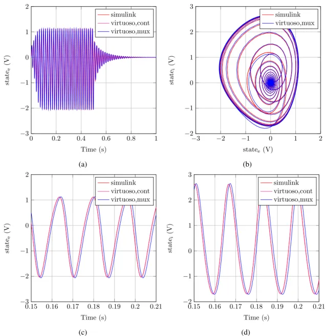
Figure 3.8 shows the response of the RKII with Kei= 1.3 and Kie= 3.8 when the input is a square wave with a period of 1 s and duty-cycle of 0.5 s, varying between 1 V and 0 V. As we can see in Figure 3.8a, when the input is 1 V, the excitatory state shows an oscillatory behavior, whereas oscillations fade when the input goes to 0 V. The same behavior is observed for the inhibitory state. It is possible to observe that the results obtained in Simulink and in Virtuoso with
0 0.2 0.4 0.6 0.8 1 −3 −2 −1 0 1 2 Time (s) state e (V) simulink virtuoso,cont virtuoso,mux (a) −3 −2 −1 0 1 2 −2 −1 0 1 2 3 statee(V) state i (V) simulink virtuoso,mux (b) 0.15 0.16 0.17 0.18 0.19 0.2 0.21 −3 −2 −1 0 1 2 Time (s) state e (V) simulink virtuoso,cont virtuoso,mux (c) 0.15 0.16 0.17 0.18 0.19 0.2 0.21 −2 −1 0 1 2 3 Time (s) state i (V) simulink virtuoso,cont virtuoso,mux (d)
Figure 3.8: Plots for one cell simulation in Virtuoso, Simulink and in Virtuoso in a multiplexed network. (a) shows the time response of the excitatory state, (b) shows the phase portrait, (c) shows oscillations in the excitatory state when the input is high, and (d) shows oscillations in the inhibitory state when the input is high.
the original model are exactly the same, and the results for the multiplexed model are very similar to them. When the input is high, the frequency of oscillation is around 61.4 Hz. In Figure 3.8b, the phase portrait obtained for the continuous model and for the discrete time model is shown. When the input is high, both models converge to a similar limit cycle, and when the input is low, both models converge to (0,0). The oscillatory response of the excitatory and inhibitory state when the input is high is better observed in figures 3.8c and 3.8d. Oscillations are equal for both continuous models, and there is a small phase difference and a small difference in amplitude between the continuous and the discrete time models.