A Software Application to Streamline and Enhance the Detection of Fraud in
Published Financial Statements of Companies
Duarte Trigueiros
University of Macau, University Institute of Lisbon Lisbon, Portugal
Email: [email protected]
Carolina Sam
Master of European Studies Alumni Association Macau, China
Email: [email protected]
Abstract—Considerable effort has been devoted to the
de-velopment of software to support the detection of fraud in published financial statements of companies. Until the present date, however, the applied use of such research has been extremely limited due to the “black box” character of the existing solutions and the cumbersome input task they require. The application described in this paper solves both problems while significantly improving performance. It is based on Web-mining and on the use of three Multilayer Perceptron where a modified learning method leads to the formation of meaningful internal representations. Such representations are then input to a features’ map where trajectories towards or away from fraud and other financial attributes are identified. The result is a Web-based, self-explanatory, financial statements’ fraud detection solution.
Keywords–Fraud Detection; Financial Knowledge Discovery; Predictive Modelling of Financial Statements; Type of Informa-tion Mining.
I. INTRODUCTION
This paper describes a software solution to help detecting fraud in published financial statements. The objective is to streamline a widely researched but scarcely used application area. Parts of the paper were presented at the Fifth Interna-tional Conference on Advances in Information Mining and Management (IMMM 2015) [1] as work-in-progress.
Fraud may cost US companies over USD 400 billion annually. Amongst different types of fraud, manipulation of published financial statements is paramount. In spite of measures put in place to detect fraudulent book-keeping, manipulation is still ongoing, probably on a huge scale [2]. Auditors are required to assess the plausibility of finan-cial statements before they are made public. Auditors apply analytical procedures to inspect sets of transactions, which are the building blocks of financial statements. But detecting fraud internally is a difficult task as managers deliberately try to deceive auditors. Most frauds stem from the top levels of the organization where controls are least effective. The general belief is that internal procedures alone are rarely effective in detecting fraud [3].
In response to concerns about audit effectiveness in detecting fraud internally, quantitative techniques are being applied to the modelling of relationships underlying pub-lished statements’ data with a view to discriminate between fraudulent and non-fraudulent cases [5]. Such external,
ex-post approach would be valuable as a tool in the hands of
users of published reports, such as investors, analysts and banks. Artificial Intelligence (AI) techniques are likewise being developed to the same end. Detailed review articles covering this research are available [6][7].
A discouraging fact is that analysts do not use tools designed to help detecting fraud in published reports. This is largely due to the fact that such tools are “black boxes” where results cannot be explained using their expertise [3]. Since analysts are responsible for their decisions, tools they may use to support decisions must be self-explanatory. Moreover, the required Extract, Transform and Load (ETL) tasks are time-consuming.
The paper aims at overcoming the above limitations. Web-mining is first employed to find, download and store data from published financial statements. Then fraud and two other attributes known to widen fraud propensity space are predicted by three Multilayer Perceptron (MLP) classifiers where a modified learning method leads to internal repre-sentations similar to financial ratios, readily interpretable by analysts. Such ratios then input a features’ map where trajectories towards or away from fraud and other financial attributes are visualized. Diagnostic interpretation is further enhanced with the display of past cases where financial attributes are similar to those being analysed.
The most valuable contribution of the application de-scribed here is its strict adherence to users’ requirements. The paper also offers a theoretical foundation for the predic-tion of financial attributes. Using such foundapredic-tion, the paper then shows that it is possible to improve significantly the ac-curacy, robustness and balance of financial statements’ fraud detection. Finally, the paper unveils an MLP training method leading to meaningful internal representations, which are capable of supporting analysts’ financial diagnostic.
Section II characterizes the issue at hand, mentions previ-ous research and lays down the foundations upon which the application is based; Section III describes the methodologies used; Section IV reports results and data used to obtain such results; Section V briefly describes the output and architecture of the application; finally, Section VI discusses limitations and benefits.
II. THEORETICALFOUNDATIONS
Fraud detection covers many types of deception: pla-giarism, credit card fraud, identity theft, medical
prescrip-tion fraud, false insurance claim, insider trading, financial statements’ manipulation and other types of fraud [8][9]. Conceptual frameworks used in the detection of, say, credit card fraud (such as Game Theory), are not necessarily efficient in detecting other types of fraud. Neural Networks are widely used in research devoted to the detection of published financial statements’ fraud [10][11][12][13][14]. The latter citation contains an extensive and updated list of papers applying analytical AI algorithms, such as the nearest neighbour classifier, Back-propagation, the Support Vector machine and others, to the detection of financial statements’ fraud and to other Financial Technology (Fin-Tech) tasks namely bankruptcy prediction.
It is pointless to compare accuracy results reported in the above-mentioned literature because samples used by authors to test such accuracy are extremely dissimilar, some being small and homogeneous while others are large and varied. Class frequencies are also imbalanced in one di-rection or in the other. Broadly, an out-of-sample overall classification accuracy of 65% to 75% is reported for large, non-homogeneous samples whereas for small, same-industry same-size samples, accuracy may be as high as 86% [14]. In all reported cases, accuracy is imbalanced: Type I and Type II errors differ by no less than 10% often being as high as 30% in both directions.
The increasing demand for Fin-Tech tools [15][16][17] has fostered the development of software to help detecting several types of fraud [18]. Tools which probe transactions for suspect patterns, as well as other internal auditing support software, are widely available but, as far as an exhaustive search may tell, the detection of fraud in published sta-tements is not on offer, probably for the reasons already stated: “black boxes” fail to meet analysts’ professional needs while the input task required by such tools would be cumbersome. Thus, evidence on published statements’ fraud detection performance is the one summarized above. In any case, claims made by vendors, even when they exist, should not be taken as evidence, especially in areas, such as the wide and fast-growing Fin-Tech market, where products seldom are the object of scientific scrutiny.
Using large, non-homogeneous data and strictly balanced random sampling, the classification precision of the appli-cation described here is 87%–88% with an imbalance of 5%. Such result is indifferently attained when using Neural Networks, Logistic regressions, C5.0, or algorithms rely-ing on Ordinary Least Squares (OLS) assumptions. While most authors emphasise comparisons between performances attained by different algorithms, in the present case the algorithm is important solely as a knowledge-discovery tool. The reported increase in performance should be credited to the use of input variables reflecting the cross-sectional characteristics of data found in financial statements. In the following, the nature of such variables is discussed.
A. Financial Analysis
Business companies, namely those listed in stock mar-kets, are required, at the end of each period, to account for their financial activity and position. To this end, companies prepare and report to the public, a collection of monetary
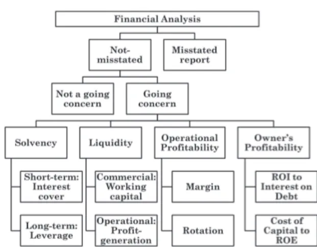
Figure 1. Hierarchical dependence of the topmost financial attributes. amounts with an attached meaning: revenues of the period, different types of expenses, asset values at the end of the period, liabilities and others. Such reports are obtained via a book-keeping process involving recognition, adjustments and aggregation into a standardised set of “accounts”, of all meaningful transactions occurring during the period. The resulting “set of accounts” is made available to the public together with notes and auxiliary information, being known as the “financial statement” of the company for that period. After being published, financial statements are routinely scrutinised by investors, banks, regulators and other entities, with the object of taking decisions regarding individual companies or industrial sectors. Such scrutiny, and the corresponding diagnostic, is known as “Financial Analysis”. Financial Analysis aims to diagnose the financial outlook of a company. The major source of data for such diagnostic is the set of accounts regularly made public by the company and by other companies in the same industrial sector. The diagnostic itself consists of identifying and in some cases measuring the state of financial attributes, such as Trustwor-thiness, Going Concern, Solvency, Profitability and others. After being identified and measured, financial attributes con-vey a clear picture of a company’s future economic prospects and may support the taking of momentous decisions, such as to buy or not to buy shares or to lend money. Financial attributes, therefore, are the knowledge set where investing, lending and other financial decisions are based.
In the hands of an experienced analyst, sets of accounts are extremely efficient in revealing financial attributes. It is possible, for instance, to accurately predict bankruptcy more than one year before the event [19]. The direction of future earnings (up or down) is also predictable [20]. Such efficiency in conveying useful information is the ultimate reason why accounts are so often manipulated by managers. Fortunately, manipulation may also be detected [4][5].
Financial analysis of a company is typically based on the comparison of monetary amounts taken from sets of accounts. The tool used by analysts to perform such compar-ison is the “ratio”, a quotient of appropriately chosen mone-tary amounts. For instance, when a company’s income at the end of a given period is compared with assets required to generate such income, an indication of Profitability emerges.
Since the effect of company size is similar in all accounts taken from the same company and period, size cancels out when a ratio is formed. Thus, by using ratios, analysts are able to compare attributes, such as Profitability, of companies of different sizes [21]. Besides their size-removal ability, ratios directly measure attributes, which are implicit in reported numbers: Liquidity, Solvency, Profitability and other attributes are associated with specific ratios. Thus, the use of ratios has extended to cases where size-removal is not the major goal. Indeed, ratios are used because they embody, to some extent, analysts’ knowledge [23]. Most analytical tasks involving accounting information require the use of appropriately chosen ratios so that companies of different sizes can be compared while their financial attributes are highlighted.
Attributes examined by financial analysts are hierarchi-cally linked: the significance and meaning of one depends on the state of others higher up in the hierarchy (Figure 1). The top attribute, which allows all the others to be meaningful, is Trustworthiness: whether a set of accounts is reliable or not. If accounts are free from manipulation, then it may be asked whether the company is a Going Concern (it is likely that the company will continue to exist) or not. Only in going concerns it makes sense to assess ratio-defined, numerical attributes, such as Solvency, Profitability and Liquidity, which also are at the root of hierarchies.
B. Ratios as model predictors
Knowledge-discovery in financial statements is the pro-cess of assigning each company in the database a set of logi-cal classes/numerilogi-cal values pertaining to attributes forming taxonomies similar to those of Figure 1. The assignment process is carried out using a corresponding set of models that, in turn, are built using “supervised learning” where algorithms learn to recognize classes from instances where diagnostics are already made; but unsupervised learning is also possible [14]. When completed, such process greatly facilitates the task of analysts, allowing them to concentrate on companies and conditions where algorithms may not be able to produce accurate diagnostics. If, however, for most of the attributes, modelling is unreliable, then knowledge-discovery is of little use. Such is the present situation, where only one of the many attributes analysts work with is accurately predictable.
As mentioned, in the hands of an experienced ana-lyst, statements published by companies reveal their fi-nancial condition. If most attempts to extract knowledge from such rich content did not succeed, it is probably due to the very success of analysts. When trying to build knowledge-discovery algorithms, authors tend to imitate analysts, namely in the use of ratios. But, in spite of being the chief tool of analysts, ratios are inadequate for knowledge-discovery: first, because their random character-istics, together with constraints they are subject to, are both unfavourable for modelling purposes; and second, because ratios are themselves knowledge, not just data.
First, ratios are inadequate because monetary amounts taken from sets of accounts, as well as their ratios, obey a multiplicative law of probabilities, not an additive law.
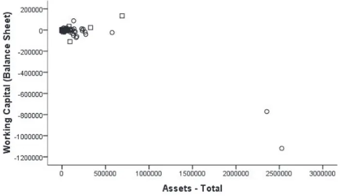
Figure 2. Influential cases in a scatter-plot of two typical ratio components. Figures reported in a given set of accounts are accumula-tions. As such, they obey a specific generative mechanism where distributions are better described by the Lognormal and other similar functions with long tails (influential cases) and inherent heteroscedasticity [21], not by the Normal, symmetrical, well-behaved distribution. Where the multi-plicative character of financial statements’ data is ignored, any subsequent effort to model such data is fruitless, not so much because OLS or other modelling and estimation assumptions are violated but due to the distorting effect of influential cases (Figure 2). And when predictive per-formance is the issue, the use of robust algorithms is not recommended because the cost of such robustness is less-ened performance. Amongst the three types of measurement, Nominal, Ordinal and Scalar, the latter is the richest in content. When scales are treated as ordered categories, as in most robust algorithms, such content is lost. Ratios are also affected by the interaction between their components, which are bounded together by book-keeping rules [22]. The numerator of several widely used ratios, for instance, is constrained to be smaller than the denominator. Such constraints, in turn, curb the variability made available to the predicting algorithm.
Second, the use of pre-defined ratios as input to most AI algorithms, namely those performing knowledge-discovery, entails a contradiction. When a ratio is chosen instead of other ratios, knowledge is required to make such choice. Each ratio embodies the analyst’s knowledge that, when two monetary amounts are set against each other, a financial attribute is evidenced. Ratios, therefore, convey previous knowledge thus limiting knowledge that may be extracted from them. Analysts use ratios because they assess one piece of information at a time. They are unable to jointly assess collections of distributions, their moments and variance-covariance matrices, as algorithms do. Analysts need focus, machines do not. Predictive models can only lose by mim-icking analysts’ separation of knowledge in small bits in order to rearrange it in a recognisable way.
In the following, adequate knowledge-discovery algori-thms are shown to be able to choose, amongst a set of monetary amounts, pairs that perform the same task as ratios. Algorithms build their own representations in a way that is similar to analysts’ task of selecting, amongst innumerable combinations of monetary amounts, the ratio that highlights
a desired attribute.
C. Cross-section characterisation of reported numbers
Studies on the statistical characteristics of reported mon-etary amounts brought to light two facts. First, in cross-section, the probability density function governing such amounts is nearly lognormal. Second, amounts taken from the same set of accounts share most of their variability as the size effect is prevalent [21]. Thus, variability of logarithm of account i from set of accounts j, log xij, is explained as
the size effect sj, which is present in all accounts from j,
plus some residual variability εi:
log xij = µi+ sj+ εi (1)
µi is an account-specific expectation. Formulations, such
as (1), as well as the underlying random mechanism, apply to accumulations only. Accounts, such as Net Income, Retained Earnings and others, that can take on both positive- and negative-signed values, are a subtraction of two accumula-tions. Net Income, for instance, is the subtraction of Total Costs from Revenue, two accumulations, not the direct result of a random mechanism.
Given two accounts i = 1 and i = 2 (Revenue and Expenses for instance) and the corresponding reported amounts x1 and x2 from the same set, the logarithm of the
ratio of x2 to x1 is
logx2
x1
= (µ2− µ1) + (ε2− ε1) (2)
It is clear why ratios formed with two accounts from the same set are effective in conveying information to analysts: the size effect, sj, cancels out when a ratio is formed. In
(2), the log-ratio has an expected value (µ2 − µ1). The
median ratio exp(µ2− µ1) is a suitable norm against which
comparisons may be made while exp(ε2− ε1) indicates the
deviation from such norm observed in j. Ratios thus reveal how well j is doing no matter its size. For instance, if the median of Net Income to Assets ratio is 0.15, any company with one such ratio above 0.15, no matter small or large, is doing better than the industry.
In (2), upward or downward deviations from the log-arithm of the industry norm are the result of subtracting two residuals, each of them account- and size-independent. The deviation ε2− ε1 from industry norms plays the crucial
role of conveying to analysts the size-independent, company-specific data they seek. It is clear, however, that ε2− ε1 is
only part of the size-independent, company-specific infor-mation available in x1 and x2. When the ratio is formed, all
variability common to x1 and x2 is removed. Residuals ε1
and ε2are uncorrelated and the size-independent,
company-specific information contained in x1and x2but not conveyed
by ε2− ε1 is the variable orthogonal to ε2− ε1, which is
ε2+ ε1[24]. Therefore, ε2+ ε1is size-independent
informa-tion not conveyed by the ratio. It is thus demonstrated that the use of ratios as model predictors curbs the information made available to the model. Only one dimension of the size-independent information, ε2− ε1, is made available while
the other dimension, ε2+ ε1, is ignored. This is yet another
disadvantage associated with the use of ratios in predictive modelling.
D. An alternative to ratios
Given this fundamental limitation of pre-selected ratios, it is worth asking whether amounts directly taken from sets of accounts would not do a better job than ratios as predictors in statistical models. Such possibility is at-tractive because predictors obeying (1) behave exceedingly well: distributions are nearly Normal, relationships are ho-moscedastic and influential cases, when present, are true outliers. Log-transformed numbers allow the use of powerful algorithms, which make the most of existing content. In the downside, one obvious concern is how to deal with accounts that can take on both positive- and negative-signed values: logarithms apply only to positive values. Another, equally pressing concern is how to keep the influence of company size out of such models: ratios are size-independent variables but log-transformed account numbers are size-dependent, indeed, most of their variability reflects just the effect of size. Finally, the interpretation of coefficients of such models would not be straightforward.
Consider the usual linear relationship where y is ex-plained by a set of predictors x1, x2, . . .
y = a + b1x1+ b2x2+· · · (3)
In the case of a Logistic regression, y may be seen as the linear score leading to the binary prediction. If, instead of x1, x2, . . . log-transformed predictors obeying (1) are
included in (3), such relationship becomes
y = A + b1ε1+ b2ε2+· · · + (b1+ b2+· · · )sj (4)
where A = a + b1µ1+ b2µ2+ . . . is a constant value and
residuals ε1, ε2, . . . now play the role of linear predictors.
The term (b1+ b2+ . . .)sj apportions the proportion of sj
(size) variability required by y. Coefficients b1, b2, . . . are
under a constraint: their summation b1+b2+. . . must reflect
the extent and sign of size-dependence in y; and where y is size-independent, b1+ b2+ . . . must assume the value of
zero so as to bar information conveyed by sj from entering
the relationship.
Suppose, for instance, that y is indeed size-independent. Moreover, y is being predicted by two accounts only, x1
and x2. In this case b2 = −b1 = b and (4) becomes y =
a + b(µ2− µ1) + (ε2− ε1) or
y = a + b logx2 x1
(5) In other words, a ratio is automatically formed so that size is removed from the relationship modelling y. Given the vari-ety of companies’ sizes found in cross-section relationships, the predictive power of sj on y is, in most practical cases,
small or non-existent. In such type of models b1+ b2+ . . .
in (4) add to nearly zero. Size-related variability is allocated to a given predictor in order to counterbalance size-related variability from other predictors, so that y is modelled by size-independent or nearly size-independent variability. When building an optimal model, the algorithm assigns the role of denominator to some predictors (negative-signed
b coefficients) and that of numerator to others
Figure 3. Graphical form where the Y-axis represents log-modulus of x. to financial ratios are thus formed. In this way, financial attributes possessing optimal predicting characteristics, are unveiled without the intervention of the analyst. This is a notable trait of the methodology.
The above reasoning presupposes that y is size-independent. By forcing the modelling algorithm to obey
b1+ b2+ . . . = 0 in (4), it is possible to build models where
y is explained solely by size-independent variability, even
in cases where the relationship is size-related. Thus, ratios are not needed to build size-independent models. Ratios are needed solely because financial analysts, and other users, demand that predictors be interpretable.
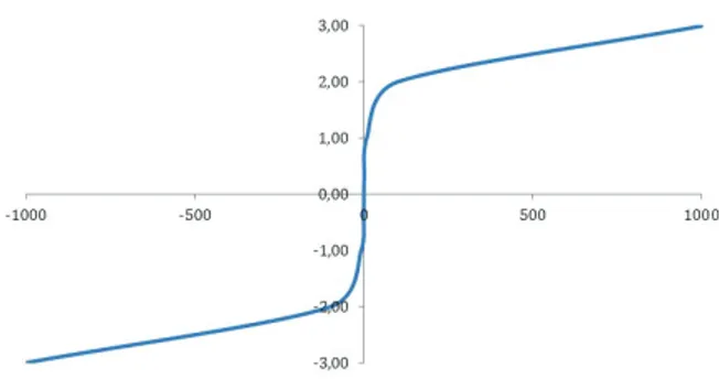
The other concern, how to deal with accounts that can take on both positive- and negative-signed values, may be solved by using the “log-modulus” [25] or other similar transformation. The log-modulus expands the logarithmic transformation so as to encompass zero and negative values. Given variable x, the log-modulus consists of using
sgn x log(|x| + 1) (6)
instead of x (Figure 3). In this way, accumulations or subtractions of accumulations, no matter their sign, become statistically well-behaved.
The log-modulus transformation considerably reduces the frequency of missing values in random samples. Missing values are a source of bias because the probability that a reported number is missing often is correlated to the attribute being predicted. For instance, it is frequent to find values of zero in Dividends and other accounts. When ratios are formed with such values in the denominator, as is the case of the ratio “Changes in Dividends in relation to the Previous Year”, a missing value is created; and such missing value is correlated with the paying or not of dividends, a predictor of future Earnings’ changes. Other changes in relation to the previous period will suffer from the same difficulty. But after the log-modulus transformation, such ratios become subtractions:
δ log x = log xt−1− log xt (7)
where t and t− 1 express subsequent time periods and the operator log may refer to (6) in the case of positive- and negative-signed x. Changes expressed as in (7) no longer increase the number of missing values. Incidentally, unlike ratios, transformed values cannot have two meanings. In ratios, negative-valued numerators and denominators lead
to the same ratio sign as positive-valued numerators and denominators.
The coming sections show that models using log-modulus transformed accounts as predictors perform better than those using ratios; but where ratios cannot be avoided, then the modelling algorithm is capable of extracting ratios with optimal predicting characteristics from logarithmic and log-modulus transformed accounts.
III. METHODOLOGY
The application described here makes use of the follow-ing methodologies: Web-minfollow-ing of financial statements; the use, as input, of logarithmic-transformed monetary amounts directly taken from such statements; pre-selection of model input variables amongst a wider set of monetary amounts; the specific architecture and training of three MLPs so that internal representations similar to financial ratios are formed; and finally, the interpretation of such MLP’s internal representations via a features’ map. This section briefly discusses such methodologies.
A. Web-mining of financial statements
Until recently, financial statements were published in a variety of formats including PDF, MS Word and MS Excel. Such variety, forced users and their supporting tools into a significant amount of interpretation and manual manip-ulation of meta-data and led to inefficiencies and costs. From 2010 on, the Securities and Exchange Commission (SEC) of the US, as well as the United Kingdom’s Revenue & Customs (HMRC) and other regulatory bodies, require companies to make their financial statements public using the XML-based eXtensible Business Reporting Language (XBRL). Users of XBRL now include securities’ regulators, banking regulators, business registrars, tax-filing agencies, national statistical agencies plus, of course, investors and financial analysts worldwide [26]. XML syntax and related standards, such as XML Schema, XLink, XPath and Names-paces are all incorporated into XBRL, which can thus extract financial data unambiguously. Communications are defined by metadata set out in taxonomies describing definitions of reported monetary values as well as relationships between them. XBRL thus brings semantic meaning into financial reporting, promoting harmonization, interoperability and greatly facilitating ETL tasks. Web-mining of financial data is now at hand.
The initial module of the application carries out Web-mining of XBRL content. The user first introduces a se-lection criteria, namely a company name or code, such as the “Central Index Key” (CIK) and the period. Then, the search of pre-existing indexes will identify Web locations containing the required statement. In the US, for instance, such location is the Securities and Exchange Commission repository (known as “EDGAR”) containing “fillings” of companies’ statements and other data.
The Electronic Data Gathering, Analysis, and Retrieval (EDGAR) repository performs automated collection, valida-tion, indexing, acceptance, and forwarding of submissions by companies and others who are required by law to file forms with the SEC. Its primary purpose is to increase the
efficiency and fairness of the securities market for the benefit of investors, corporations, and the economy by accelerating the receipt, acceptance, dissemination, and analysis of time-sensitive corporate information filed with the agency. The SEC’s File Transfer Protocol (FTP) server for EDGAR filings allows comprehensive access by corporations, funds and individuals.
The actual annual statement of companies need not be submitted on EDGAR, although some companies do so voluntarily. However, a report on a standardised format, known as “Form 10-K”, which contains much of the same information, is required to be filed on EDGAR; and since recently filers are also required to submit documents in XBRL format. Besides the 10-K form, other widely used form is the 10-Q, which refers to quarterly statements. Rules established by the SEC offer guidelines for the content and format, including which data may be provided as part of an Interactive Data document, and the relationship to the related official filing.
An extremely helpful resource for FTP retrieval is the set of EDGAR indices listing the following information for each filing: company name, form type, CIK of the company, date filed, and file name (including folder path). Four types of indexes are available:
1) company, sorted by company name 2) form, sorted by form type, 10-K or 10-Q 3) master, sorted by CIK code
4) XBRL, list of submissions containing XBRL finan-cial files, sorted by CIK code.
The application described here uses the package “XBRL” from the R language [27] to access and retrieve SEC filings. The XBRL package offers access to functions to extract business financial information from a XBRL instance file and the associated collection of files that defines its Discoverable Taxonomy Set (DTS).
When the report from a given company and period is re-quested by a user, an index is searched and the corresponding document is retrieved from its Web location on EDGAR. Next, the relevant information is put in place. Functions provided by the XBRL package return readily available data, complete with standard descriptions, including taxonomies. As published taxonomy files are immutable and are used by most filers, the package offers the option of downloading them only the first time they are referred, keeping a local cache copy that can be used from then on.
B. Data description and variable selection
Financial analysts base their diagnostic on several con-curring pieces of evidence, in favour or against a priori hy-potheses. On the other hand, the extant research on financial statements’ manipulation suggests that fraudulent numbers lead to detectable imbalances in financial features. For instance, income may increase without the corresponding increase in free cash. In order to respond to the need, in the part of analysts, to examine concurring facts, the application, besides predicting fraud, also predicts the state of two other attributes mentioned in published research [4][5] as capable of detecting such imbalances.
Therefore, after Web-mining and the log-transformation of monetary amounts as described in Subsection II-D, three MLP are set to separately predict three financial attributes known to widen fraud propensity space, namely:
• Trustworthiness, comprising two classes (states): fraudulent (manipulated, misstated) vs non-fraud-ulent statement [4][5][7];
• Going Concern, comprising two classes: bankrupt vs solvent [19][28][29];
• Unexpected Increase in Earnings One Year Ahead, comprising two classes: Earnings’ increase vs Earn-ings’ decrease one year ahead [20][30].
Trustworthiness and Going Concern are the two basic at-tributes of financial analysis, directly influencing the way all other attributes are interpreted. As for Earnings’ direction one year ahead, it is, amongst the attributes occupying a place further down in the hierarchy, one often scrutinized by investors.
So far, Going Concern is the only predictable attribute. In spite of the large research effort devoted to improving Trustworthiness prediction, until now, as mentioned, results are below the feasibility level, at 75% out-of-sample correct classification at best, for large, non-homogeneous samples. Besides being meagre, such results are unbalanced: one of the states is significantly better predicted than the other. All the previously cited authors use ratios as predictors.
Instances employed in the training and testing of the three MLP and the corresponding input and target attributes are extracted from the following sources:
• UCLA-LoPucki Bankruptcy Research Data [31] as well as a list of bankrupt companies kindly provided by Professor Edward Altman (New York Univer-sity), covering the period 1978-2005.
• The collection of Accounting and Auditing Enforce-ment Releases (AAER) resulting from investigations made by the SEC against a company, an auditor, or an officer for alleged accounting and/or auditing misconduct, identifying a given set of accounts as fraudulent [5], covering the period 1983-2013. This data is made available by the Centre for Financial Reporting and Management of the Haas School of Business (University of California at Berkeley) [32].
• The “Compustat” repository of financial data by Standard & Poor’s, where monetary amounts are collected, and from which unexpected Earnings in-creases and dein-creases are estimated [20][30]. Input to each of the three MLP are logarithms or log-modulus, (6), of accounts pre-selected amongst all the aggre-gated accounts in published statements. Accounts are taken from two consecutive statements of a company, forming instance j of actual period, t, and of previous period, t− 1. Log-differences in relation to such previous period, (7), are computed and included in the pre-selection process.
Pre-selection of input variables is carried out using the “Forward Selection” algorithm attached to most Logistic regressions [33]. Accounts and log-differences selected in this way are then used as input to the corresponding MLP.
TABLE I. BK= BANKRUPTCY, FR= FRAUD, EA= EARNINGS.
Log Cash and Short Term Investments Bk Fr Log Receivables (total) Fr Log Assets (total) Fr Ea Log Long-Term Debt Fr Log Liabilities (total) Bk Fr Ea Log Liabilities (total) change Fr Lmd Retained Earnings Bk Ea Lmd Retained Earnings change Ea Log Common Stock (equity) Fr Log Revenue (total) Fr
Lmd Gross Profit Ea
Lmd Gross Profit change Ea
Lmd Tax Expense Bk Ea
Lmd Cash-Flow from Operations Bk Ea Lmd Dividends per Share Ea Lmd Dividends per Share change Ea
Table I lists the 16 variables that were pre-selected using such method, together with the attribute they predict and the type of transformation applied in each case: “log” for the logarithmic transformation (positive-only accounts) and “lmd” for the log-modulus transformation (accounts which may take both positive and negative values).
C. MLP architecture and training
When analysing attributes, such as Trustworthiness, fi-nancial analysts need to know which ratios are at work, their position in relation to industry standards and in which direction they are moving. In order to respond to the first of such demands, MLP architecture and training are designed so that internal representations similar to financial ratios are formed in hidden nodes. Before training, MLP architecture consists of:
1) A total of 41 input nodes corresponding to the 16 variables listed on Table I plus 24 dummies, one for each of the “Global Industry Classification Stan-dard” (GICS) groups [34] (each instance belongs to one such industrial group), plus a constant-valued dummy.
2) one hidden layer with 10 nodes in each of which an internal representation similar to a ratio may be formed;
3) two output nodes where outcomes are symmetrical about zero, plus the corresponding “biases” as-signed to the constant value of 1 and -1. Symmetry and output node duplication is not required, in theory, but it may facilitate training.
Hyperbolic tangents (threshold functions symmetrical about zero) are used as transfer functions in all nodes.
Given the inclusion of 24 dummies, hidden nodes’ biases assigned to the constant value of 1 should be redundant. But since, during training, MLP connections (weights) are subject to a stringent pruning whereby most connections disappear, the constant bias often is the sole remaining dummy.
MLP training is carried out in the usual way until a minimum is found. Then a popular weight pruning technique known as “Optimal Brain Surgeon” [35] is applied. The result is a significant reduction in the number of connections. Typically, all of the industry dummies, plus a significant number of input variables and, often, entire hidden-layer nodes are discarded at this stage.
Figure 4. Given values xk and xi, the ratio xkj/xijfrom statement j, is formed in an MLP hidden node as log xkj− log xijwhen wk=−wi. The next training step consists of an extremely crude penalisation of synaptic weights linking inputs, the log xiin
(1), to hidden nodes: each epoch reduces the absolute value of weights by a small margin, typically 0.001. This leads to a kind of competition for survival amongst weights; and it is verified that some weights are resilient in the sense that they regain their values while others are non-resilient, quickly decaying to zero, and are pruned.
Then, beginning with the most significant node, all but the two largest-valued input weights are pruned. The pruning is repeated in the other nodes, one at a time, while synaptic weights linking input variables to all hidden nodes keep on being subject to the described penalisation. When the relationship being modelled is strong, as is the case of bankruptcy prediction, this procedure is sufficient to bring about internal representations similar to ratios; in the case of weak relationships, the procedure requires trial and error in the choice of the first hidden nodes to be subject to the forced pruning of all but two weights.
Instances used in MLP training greatly differ in size while the predicted variable is indeed predictable. Hidden nodes, therefore, have a tendency towards self-organizing themselves into size-independent variables, which are, at the same time, efficient in explaining the attribute being modelled. This is basically the definition of a financial ratio; and the described procedure simply avoids ratios with more than one numerator and denominator.
According to (5), in a nearly size-independent predicting context, synaptic weights tend to survive in each node so that their summation is nearly zero. And if nodes are further forced into having two weights only, then such two weights will be symmetrical (opposite signs and approximately sim-ilar absolute values). Internal representations thus mimic the logarithm of ratios and can be interpreted similarly to ratios (Figure 4). Note that the term “internal representation” refers to values assumed by each hidden node after summation (SUM in Figure 4) but before transfer function.
In some hidden nodes, only one weight survives, not two. This may happen where input variables are themselves ratios, such as Dividends per Share or changes from the previous- to the current-year account (7). This may also happen when the relationship to be modelled requires the presence of size as a predictor.
Although absolute values of the two surviving weights in each hidden node are not much different from one another, they differ across nodes. Such difference, together with the magnitudes of synaptic weights linking them to output nodes, crudely reflects the importance of each node for the final classification performance. In the final step of training,
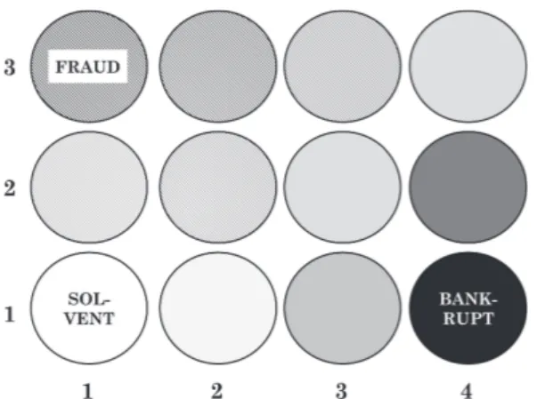
Figure 5. Position of financial attributes’ classes in 4 by 3 features’ map. the less important hidden node is also tested for pruning us-ing trial and error, the prunus-ing criterion beus-ing non-significant reduction in performance. The final result is a parsimonious model with meaningful internal representations.
After appropriate ratios are selected, analysts interpret their observed, company-specific deviations from expecta-tion. In this way, expected µi from (1) are also modelled
and accounted for inside such node. Since node outputs and attributes’ classes are both balanced, the effect of industry dummies is to subtract industry-specific log-ratio standards from internal representations thus making them similar to a difference of two εi in (1). Such difference is, in log
space, what analysts seek when they compare a ratio with its expectation. As mentioned, for the modelling tasks at hand, industry dummies are not significantly distinctive.
D. Graphical interpretation of results
Internal representations from the three MLP are input to a 2-dimensional features’ map [36] with 4 by 3 nodes. When self-organisation has taken place, specific nodes or groups of nodes in the map become associated with classes of attributes, such as fraud and bankruptcy (Figure 5). Visual examination of the features’ map facilitates interpretation, both proximity to a given node and trajectories towards or away from nodes, being informative. In this way, analysts observe in which direction attributes move and whether a company is approaching nodes where fraud, bankruptcy and unexpected changes in Earnings are likely.
The self-organised map aims at facilitating the graphical interpretation of representations created by the three MLP; no inferential role is attributed to it.
IV. RESULTS
For the three MLP, this section lists the input weights which survive pruning, the ratios formed from them in hidden layers and their relative importance for explaining the outcome. Test-set classification accuracy is also reported. MLP performance is compared with that of Logistic regres-sion classifiers using similar data-sets and MLP’s surviving inputs as predictors. In this way, the performance of models using the newly discovered ratios as predictors is compared with that of models using ratio components as predictors. The section concludes by showing the self-organised fea-tures’ map at work.
A. Bankruptcy prediction
From a total of 2,997 cases of US bankruptcy filings, and after discarding bankruptcies but the first in each company as well as cases about which detailed financial figures are not available, two random samples of nearly 900 different cases each are drawn. The two samples contain companies listed in US exchanges and present in the Standard & Poor’s “Compustat” database. They span the period 1979-2008. The deciles of the logarithm of Assets (total) are used as a discrete size measure, all sizes being represented in samples. Similarly, all the 24 GICS groups are significantly represented in samples. Cases in the two samples are then matched with an equal number of records from non-bankrupt companies. Pairing is based on the GICS group, on size decile and on year. Among financial statements fulfilling the pairing criteria, one case is randomly selected for matching and then such case is made unavailable for future matching. Although the same case is not used to match more than one bankruptcy case, other cases from the same company in different years remain available for matching. The two matched samples have nearly 1,800 cases each. One of the two samples, always the same, is used as the learning-set and the other as the test-set. Due to missing observations, samples contain less than 1,800 cases:
Learning-set: non-bankrupt 845 (50.1%) Learning-set: bankrupt 841 (49.9%) Test-set: non-bankrupt (N) 837 (49.8%) Test-set: bankrupt (P) 845 (50.2%)
When the MLP learning process is concluded, only 4 hidden nodes persist. In each of these, the two input weights which survive pruning are of a crudely similar magnitude and opposite sign. Therefore, the MLP has formed 4 internal representations, B1 to B4, which are similar to financial ratios in log space. When ordered by magnitude of the weight leading to output nodes, a rough measure of pre-dictive importance, such ratios are:
B1 ratio of Cash and Short Term Investments to Liabilities (total)
B2 ratio of Retained Earnings to Liabilities (total) B3 ratio of Cash-Flow from Operations to Cash and
Short Term Investments
B4 ratio of Tax Expenses to Liabilities (total) All industry-specific weights are also pruned away during training, denoting no significant influence of the industrial group on bankruptcy prediction. Therefore, the final MLP model has 5 inputs (detailed in Table I), 4 hidden nodes and 2 symmetrical but otherwise identical outputs.
Test-set performance of the MLP using the above 4 log ratios (internal representations) formed from 5 inputs, is reported in Table II together with the performance of a Logistic regression using the same 5 inputs as predictors.
As mentioned, bankruptcy prediction is the sole case of successful modelling of financial attributes. This is probably due to the fact that statements were perfected so as to warn against solvency problems. Therefore, the relationship is strong. Performance reported here is not inferior to that found in the literature while balance increases markedly.
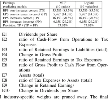
TABLE II. BANKRUPTCY PREDICTION CLASSIFICATION RESULTS.
Bankruptcy MLP Logistic predicting models (4 ratios) (5 variables) Non-bankrupt correct (TN) 822 (98.2%) 822 (98.2%) Non-bankrupt incorrect (FP) 15 (1.8%) 15 (1.8%) Bankrupt correct (TP) 811 (96.0%) 814 (96.3%) Bankrupt incorrect (FN) 34 (4.0%) 31 (3.7%) Precision: TP / (TP + FP) 98.18% 98.19%
The number of variables and synaptic weights engaged in modelling is less than that reported in the literature. Robustness is therefore higher. When predictors are ratio components rather than ratios (Logistic regression), perfor-mance increases slightly.
B. Fraud detection
The methodology used in the building of fraud-detecting samples is similar to the bankruptcy-prediction case. Data used for learning and testing consists of a collection of 3,403 AAERs. It contains enforcement releases issued be-tween 1976 and 2012 against 1,297 companies, which had manipulated financial statements. After removing cases for which no detailed financial data is available, the database contains 1,152 releases. Manipulated statements from the same company in different years are not removed from the sample. Enron, for instance, was the object of 6 releases and all of them are included. Two random samples of nearly 550 different cases each are then drawn. They span the period 1976-2008. All sizes and all GICS groups are significantly represented. The two samples are matched with an equal number of statements from companies that are neither the object of releases throughout the period nor bankrupt in the year of the release. Matched samples have nearly 1,100 cases each. One of the two samples, always the same, is used to build models and the other to test performance of models. Due to missing observations, the size of samples available for model-building and model-testing ends up being less than 800 cases each:
Learning set: non-fraud cases 335 (45.7%) Learning set: fraud cases 398 (54.2%) Test set: non-fraud cases (N) 353 (46.2%) Test set: fraud cases (P) 411 (53.8%)
When the MLP learning process is concluded, 6 hidden nodes persist. Five of these 6 nodes have two surviving input weights with a relatively similar magnitude and opposite sign. The remaining node, F5, has only one surviving weight. The MLP has formed 5 internal representations, F1 to F4 plus F6, which are similar to financial ratios in log space. The following list displays the representations in the 6 hidden nodes ordered by magnitude of weight leading to the output node, a rough measure of predictive importance:
F1 ratio of Liabilities (total) to Assets (total) F2 ratio of Cash and Short Term Investments to
Revenue (total)
F3 ratio of Long Term Debt to Common Stock (equity)
F4 ratio of Receivables (total) to Common Stock (equity)
F5 Change in Liabilities (total)
F6 ratio of Revenue (total) to Common Stock
(eq-TABLE III. FRAUD DETECTION CLASSIFICATION RESULTS.
Fraud MLP Logistic
predicting models (6 ratios) (8 variables) Non-fraud correct (TN) 299 (84.7%) 303 (85.8%) Non-fraud incorrect (FP) 54 (15.3%) 50 (14.2%) Fraud correct (TP) 369 (90.0%) 371 (90.5%) Fraud incorrect (FN) 41 (10.0%) 39 (9.5%) Precision: TP / (TP + FP) 87.2% 88.1% uity)
All industry-specific weights are pruned away during train-ing. Therefore, the final MLP model has 8 inputs (detailed in Table I), 6 hidden nodes and 2 symmetrical but otherwise identical outputs.
Test-set performance of fraud-detecting MLP using 8 inputs and 6 hidden nodes is reported in Table III together with the performance of the Logistic regression using the same 8 inputs. The model shows a substantial increase in out-of-sample performance, of more than 10% in relation to previous studies using large, diversified samples, while imbalance in the recognition of classes is reduced. Type II error (the most expensive in this case) is clearly subdued. When predictors are ratio components rather than ratios (Logistic regression), performance increases.
C. Earnings prediction
The task of predicting Earnings’ changes one year ahead is generally considered as having theoretical rather than practical interest: it is indeed possible to predict Earnings but, so far, the attained increase in accuracy over the tossing of a coin is barely 10% [20].
Samples used in the prediction of the sign of unexpected changes in Earnings (in fact Earnings per Share, EPS) one year ahead, are not matched: classes to be predicted are estimated from data available in each set of accounts [20]. In the present case, after withdrawing cases with missing values in the predicted dichotomous variable (Earnings increase vs Earnings non-increases) or in predictors, a total of nearly 140,000 cases remain, where some 90,000 are non-increases and 50,000 are increases. The size of the sample is higher than in previous cases and classes are unbalanced: after adjusting for expectation, non-increases are more frequent than increases. Other methodological details are the same as in previous cases. The final number of cases in the learning-and test-set is:
Learning set: EPS non-increases 41,851 (64.3%) Learning set: EPS increases 23,275 (35.7%) Test set: EPS non-increases (N) 41,750 (64.4%) Test set: EPS increases (P) 22,811 (35.6%)
Class proportions are significantly dissimilar in this case. When the MLP learning process is concluded, 10 hidden nodes persist, 5 of which have only 1 synaptic weight. In the remaining 5 nodes the two surviving input weights are of a relatively similar magnitude and opposite sign. The MLP has formed 5 internal representations, E2, E3, E5, E6 and E7, which are similar to financial ratios in log space. The following list displays the 10 representations formed in hidden nodes ordered by the magnitude of weight leading to the output node, a rough measure of predictive importance:
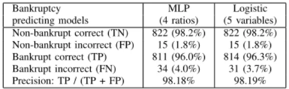
TABLE IV. EARNINGS PREDICTION CLASSIFICATION RESULTS.
Earnings MLP Logistic
predicting models (10 ratios) (10 variables) EPS non-increases correct (TN) 35,783 (85.7%) 35,783 (85.7%) EPS non-increases incorrect (FP) 5,967 (14.3%) 5,967 (14.3%) EPS increases correct (TP) 16,153 (70.8%) 16,153 (70.8%) EPS increases incorrect (FN) 6,658 (29.2%) 6,658 (29.2%) Precision: TP / (TP + FP) 73.02% 73.02%
E1 Dividends per Share
E2 ratio of Cash-Flow from Operations to Tax Expenses
E3 ratio of Retained Earnings to Liabilities (total) E4 Change in Gross Profit
E5 ratio of Retained Earnings to Tax Expenses E6 ratio of Gross Profit to Cash Flow from
Oper-ations E7 Assets (total)
E8 ratio of Tax Expenses to Assets (total) E9 Change in Retained Earnings
E10 Change in Dividends per Share
All industry-specific weights are pruned away. The final MLP model has 10 inputs (detailed in Table I), 10 hidden nodes and 2 symmetrical but otherwise identical outputs.
Test-set performance of the MLP Earnings-predicting model using the 10 input just mentioned, is reported in Table IV together with the performance of the Logistic regression model using the same 10 inputs differently organ-ised: instead of ratios, ratio components are used as input. Performance is, in this case, similar for ratios (MLP) and their components (Logistic regression).
One of the internal representations is not a ratio but the logarithm of Assets (total). This introduces in the modelling of Earnings’ changes the effect of size, required by this particular relationship.
Classification results should be interpreted in the light of the strong class imbalance observed in the training-set [37], which is nearly 14% in this case. Namely, a classification accuracy of 73%, obtained from an initial class imbalance of 14% means a gain, in relation to a classifi-cation made at random (without any previous information) of 9% = 73% − (50% + 14%). Contrary to published results [20][30], the final classification imbalance is not worsened by the modelling process. In the present case, imbalance is similar to that of the sample used to build models while performance is significantly increased by 4% in relation to such previously reported performance.
D. The features’ map
Data employed to self-organise the features map con-tains instances used in the learning and testing of two of the MLP, namely bankruptcy-prediction and fraud-detection data. Classes, such as fraud, bankruptcy and their opposites may occur together in some instances; and all instances include the two classes of unexpected Earnings’ increases and decreases. The total number of instances is 5,369.
When self-organised, the 4 by 3 nodes in the features’ map are sensitive to distinct financial attributes. Considering the lattice of 12 nodes defined as x, y where x = 1, . . . 4 and y = 1, . . . 3, the strongest sensitivities observed are as follows:
• Fraud in node x = 1, y = 4
• Bankruptcy in node x = 4, y = 1 and its opposite, Solvency, in node x = 1, y = 1
• Earnings’ decrease in nodes x = 1, y = 1 and x = 1, y = 3
Figure 6 compares the frequencies associated with, respec-tively, fraud, bankruptcy and unexpected Earnings’ decreases in the self-organised map.
Besides graphically locating the financial position of companies with reference to fraud and bankruptcy, the self-organised features’ map shows the trajectory drawn by companies, from the previous into the current year. Figure 7 illustrates the yearly evolution of the accounts of some, well-known, financial scandals and failures, as mapped into the self-organised lattice.
V. ARCHITECTURE, OUTPUT ANDDEPLOYMENT The most informative result provided by the application is the set of three probabilities obtained from MLP outputs. After being adjusted so as to become 0-1 variables, such outputs may be interpreted as conditional probabilities of ob-serving the associated input values when the predicted class is fraud, bankruptcy and Earnings decrease respectively. And when combined with Prevalence numbers (prior probabilities of fraud, bankruptcy and Earnings decrease), MLP outputs become posterior probabilities of fraud, bankruptcy or Earn-ings decrease given the values observed in input variables. Posterior probabilities are then made available to users as outputs. Output node representations (after summation but before the transfer function) can also be used as scores.
Each analysed company generates two sets of results corresponding to time periods t−1 and t. Output to analysts consists of the following:
1) Three posterior probabilities: fraud, bankruptcy and Earnings’ decrease, with a sign indicating the di-rection of their change from t− 1 to t.
2) The respective scores.
3) The 9 most significant values internal representati-ons assume at period t, three from each MLP, with a sign indicating the direction of change from t−1 to t. Values are labelled as the respective ratio. 4) Graphical description of financial position in the
self-organised features’ map and trajectories from
t− 1 to t, allowing the detection of trends towards
a given class.
5) Names, year and attributes of three instances from the learning- and test-set, which are closest to the instance being investigated respectively regarding fraud, bankruptcy and unexpected Earnings’ de-crease. The proximity criterion used in the three cases is the value of the internal representation formed in one of the output nodes.
The application uses a variety of packages and languages, namely the R-language; it has been set-up, tested and deployed in two versions, stand-alone and Web-based, the latter having no training capability. The stand-alone version is a Java-based set of modules, as depicted in Figure 8.
Figure 6. Class frequencies in features’ map. Node x = 4, y = 1, bankruptcy; node x = 1, y = 3, fraud; nodes x = 1, y = 1 to 3, Earnings’ decreases.
Figure 7. Trajectories drawn by well-known cases in the features’ map.
VI. CONCLUSION
Notwithstanding the abundance of research devoted to the subject, until now, the surge in marketed Financial Tech-nology applications did not contemplate software to support the detection of fraud in published financial statements. This is due to difficulties in extracting and put in place of the required input data and also due to the “black box” nature of researched solutions. The application presented here aims at solving both problems, producing automated Web-mined input and interpretable diagnostics. In the hands of analysts, the application’s output is self-explanatory, not just pointing out companies likely to have committed fraud but showing, rather than hiding, financial attributes that are capable of supporting such diagnostic.
Limitations of ratios highlighted in the paper, some of which persist after appropriate logarithmic or log-modulus transformations, are not sufficient to erode performance sig-nificantly. Experiments reported in the paper show that log-ratio use, as an alternative to log-transformed accounts, is acceptable for predictive modelling purposes. This probably stems from the fact that such log-ratios are discovered by the optimisation algorithm, rather than being pre-selected by analysts. In this way, the most performance-damaging ratios will not be selected, meaningful as they may seem to be. Ra-tios, in turn, bring with them some noteworthy advantages, namely diagnostic interpretability and size-independence, including much needed currency-independence.
The application illustrates a case of close alignment
Figure 8. Modular architecture of the stand-alone application deployed. between users’ needs and algorithmic characteristics. The application is also an example of knowledge-discovery, whereby explanatory variables are discovered amongst many candidates so that a predicting task is carried out with optimal performance. The choice of the algorithm, the MLP, was dictated solely by its ability to form meaningful internal representations. Neither algorithmic performance nor the testing of novel algorithmic capabilities was the goal here. Out-of-sample classification results obtained are more than 10% above those reported by other authors for large-non-homogeneous samples; but such increase in performance is obtained simply by using, as input variables, log-transformed accounts rather than previously-defined ratios. Appropriately transformed variables, not algorithms, led to the discovery of log-ratios and then to parsimonious, precise, balanced and robust prediction.
The final goal is to build a usable tool, an apparently simple task but which, in this particular subject area, has eluded research effort during the last 20 years. Thus, the ultimate test is yet to be carried out, namely whether analysts will use the application or not.
ACKNOWLEDGMENTS
This research is sponsored by the Foundation for the Development of Science and Technology (FDCT) of Macau, China.
REFERENCES
[1] D. Trigueiros and C. Sam, “Streamlining the Detection of Accounting Fraud through Web Mining, and Interpretable Internal Representati-ons,” in Proc. IMMM 2015: The Fifth International Conference on Advances in Information Mining and Management, Brussels, June 2015, pp. 23–26, ISBN: 978-1-61208-415-2.
[2] M. Nigrini, Forensic Analytics: Methods, and Techniques for Foren-sic Accounting. John Wiley, and Sons, 2011.
[3] W. Albrecht and M. Zimbelman, Fraud Examination. Mason, South-Western Cengage Learning, 2009.
[4] M. Beneish, “The Detection of Earnings Manipulation,” Financial Analysts Journal, vol. 55, no. 5, pp. 24–36, 1999.
[5] C. Dechow, G. Weill, and R. Sloan, “Predicting Material Accounting Misstatements,” Contemporary Accounting Research, vol. 28, no. 1, pp. 17–82, 2011.
[6] E. Ngai, Y. Hu, Y. Wong, Y. Chen, and X. Sun, “The Application of Data Mining Techniques in Financial Fraud Detection: a Classifica-tion Framework, and an Academic Review of Literature,” Decision Support Systems, vol. 50, no. 3, pp. 559–569, 2011.
[7] A. Sharma and P. Panigrahi, “A Review of Financial Accounting Fraud Detection Based on Data Mining Techniques,” International Journal of Computer Applications, vol. 39, no. 1, 2012.
[8] K. Phua, V. Lee, and R. Gayler, “A Comprehensive Survey of Data Mining-Based Fraud Detection Research,” Clayton School of Information Technology, Monash University, 2005.
[9] U. Flegel, J. Vayssire, and G. Bitz, “A State of the Art Survey of Fraud Detection Technology,” in Insider Threats in Cyber Security, ser. Advances in Information Security, C. W. Probst, J. Hunker,, and M. Bishop, Eds. Springer US, vol. 49, pp. 73–84, 2010.
[10] E. Kirkos, S. Charalambos, and Y. Manolopoulos, “Data Mining Techniques for the Detection of Fraudulent Financial Statements,” Expert Systems with Applications, vol. 32, p. 995–1003, 2007. [11] W. Zhou and G. Kapoor, “Detecting Evolutionary Financial
State-ment Fraud,” Decision Support Systems, vol. 50, pp. 570–575, 2011. [12] P. Ravisankar, V. Ravi, G. Rao, and I. Bose, “Detection of Financial Statement Fraud, and Feature Selection Using Data Mining Tech-niques,” Decision Support Systems, vol. 50, no. 2, pp. 491–500, 2011.
[13] F. Glancy and S. Yadav, “A Computational Model for Financial Reporting Fraud Detection,” Decision Support Systems, vol. 50, no. 3, pp. 595–601, 2011.
[14] S. Huang, R. Tsaih, and F. Yu, “Topological Pattern Discovery and Feature Extraction for Fraudulent Financial Reporting,” Expert Systems with Applications, vol. 41, no. 9, pp. 4360–4372, 2014. [15]
https://www.quora.com/What-are-the-biggest-FinTech-trends-in-2015 Retrieved: May 2016.
[16] http://blog.dwolla.com/12-companies-pushing-fintech/ Retrieved: May 2016.
[17] https://letstalkpayments.com/applications-of-machine-learning-in-fintech/ Retrieved: May 2016.
[18] http://www.capterra.com/financial-fraud-detection-software/ Re-trieved: May 2016.
[19] E. Altman, “Financial Ratios, Discriminant Analysis, and the Pre-diction of Corporate Bankruptcy,” The Journal of Finance, vol. 23, no. 4, pp. 589–609, 1968.
[20] J. Ou and S. Penman, “Financial Statement Analysis, and the Prediction of Stock Returns,” Journal of Accounting, and Economics, vol. 11, no. 4, pp. 295–329, 1989.
[21] S. McLeay and D. Trigueiros, “Proportionate Growth, and the Theoretical Foundations of Financial Ratios,” Abacus, vol. XXXVIII, no. 3, pp. 297–316, 2002.
[22] D. Christodoulou and S. McLeay, “The Double Entry Constraint, Structural Modeling and Econometric Estimation,” Contemporary Accounting Research, vol. 31, no. 2, pp. 609–628, 2014.
[23] W. Beaver, “Financial Ratios as Predictors of Failure,” Journal of Accounting Research, Suplement. Empirical Research in Accounting: Select Studies, vol. 4, pp. 71–127, 1966.
[24] D. Trigueiros, “Incorporating Complementary Ratios in the Analysis of Financial Statements,” Accounting, Management, and Information Technologies, vol. 4, no. 3, pp. 149–162, 1994.
[25] J. John and N. Draper, “An Alternative Family of Transformations,” Journal of the Royal Statistical Society, Series C (Applied Statistics), vol. 29, no. 2, pp. 190–197, 1980.
[26] T. Dunne, C. Helliar, and R. Mousa, “Stakeholder Engagement in Internet Financial Reporting: The diffusion of XBRL in the UK,” The British Accounting Review, vol. 45, no. 3, pp. 167–182, 2013. [27] R. Bertolusso and M. Kimmel, “XBRL: Extraction of Business Financial Information from XBRL documents,” 2015, CRAN repos-itory, https://cran.r-project.org/web/packages/XBRL/index.html Re-trieved: May 2016.
[28] E. Altman, Corporate Financial Distress. Wiley (New York), 1983. [29] M. Bellovary and D. Giacomino, “A Review of Bankruptcy
Predic-tion Studies: 1930-present,” Journal of Financial EducaPredic-tion, vol. 33, pp. 1–42, 2007.
[30] J. Ou, “The Information Content of Non-Earnings Accounting Numbers as Earnings Predictors,” Journal of Accounting Research, vol. 28, no. 1, pp. 144–163, 1990.
[31] http://lopucki.law.ucla.edu/ Retrieved: May 2016.
[32] http://groups.haas.berkeley.edu/accounting/faculty/aaerdataset/ Re-trieved: May 2016.
[33] D. Trigueiros and C. Sam, “Log-modulus for Knowledge Discovery in Databases of Financial Reports.” in Proc. IMMM 2016: The Sixth International Conference on Advances in Information Mining and Management, Valencia, May 2016, pp. 26–31, ISBN: 978-1-61208-477-0.
[34] https://www.msci.com/gics Retrieved: May 2016.
[35] G. Hassibi and D. Stork, “Optimal Brain Surgeon, and General Network Pruning,” in Proc. IEEE International Conference on Neural Networks, San Francisco, CA, 1993, vol. 1, pp. 293–299. [36] T. Kohonen, Self-Organization, and Associative Memory. Springer
Verlag (Berlin), 1984.
[37] N. Chawla, “Data Mining for Imbalanced Datasets: an Overview,” in Data Mining, and Knowledge Discovery Handbook, O. Maimon, and L. Rokach, Eds. Springer US, pp. 853–867, 2005.