Vol. 34, No. 03, pp. 775 – 788, July – September, 2017 dx.doi.org/10.1590/0104-6632.20170343s20150490
* To whom correspondence should be addressed
STUDY OF CONTINUOUS RHEOLOGICAL
MEASUREMENTS IN DRILLING FLUIDS
S. da C. Magalhães Filho
1*, M. Folsta
2, E. V. N. Noronha
1,
C. M. Scheid
1and L. A. Calçada
11Department of Chemical Engineering, Federal Rural University of Rio de Janeiro, BR 465, km 7, 23890-000 Seropédica, Brazil,
*E-mail: [email protected]; [email protected]
2PETROBRAS S.A/CENPES, Humavenue, Square 07, Ilha do Fundão, 21494-000 Rio de Janeiro, RJ, Brazil.
(Submitted: August 4, 2015; Revised: April 14, 2016; Accepted: April 17, 2016)
Abstract – Drilling an oil well involves using drilling fluids that perform cleaning and cooling functions, but that
most importantly maintain the fluids of the geological formation contained by hydraulic pressure. A fundamental role in predicting the hydraulic pressure of the well consists of monitoring the fluid’s rheological behavior. This paper summarizes an ongoing effort to measure, by evaluating the performance of two online viscometers, drilling fluids’ rheological behavior in real time. One online method proposes a modified Couette system. The other consists of a standard pipe viscometer with default modeling. The performances of the online devices were compared with an offline method – a Couette device commonly used in oilfields as a benchmark. For Newtonian fluids, agreement between the rheological behaviors was found for all instruments, validating the methodology proposed. For non-Newtonian fluids,
there were divergences, which were investigated and their probable causes determined to be the following: homogeneity,
slippage effects, and interaction in the fluid/gap interfaces. A case study demonstrated that these divergences were not significant during the prediction of hydraulic pressure, meaning that the methodology proposed has the potential to
improve overall drilling performance.
Keywords: drilling fluid, online rheology, automation, continuous measurement.
INTRODUCTION
Drilling petroleum wells in ultra-deep water is an operation of great cost and risk. Due to the extreme pressure and temperature conditions, the operational window of hydraulic pressure control is too narrow for mistakes. This window represents the minimum and maximum pressures that can be applied to the system so
as to avoid undesired flows towards the well, such as water
or gas invasion originating from the rocks. The minimum pressure is known as porous pressure and the maximum is known as fracture pressure (Shaughnessy et al., 2007). To maintain the hydraulic pressure within the limits of the porous and fracture pressures, a common technique is the
overbalanced technique. (In fact, the majority of Brazilian petroleum wells have been drilled in this manner.) In this
technique, the operator pumps a drilling fluid throughout
the well. To control the hydraulic pressure, it is necessary to
characterize the rheological behavior of the fluid. Without
such a parameter, it is impossible to predict hydraulic pressure and consequently maintain control.
In oilfields, operators carry out rheological measurements using offline viscometers that make use of
manual procedures which date back more than 50 years. The evaluation of this process can be enhanced with online measurements. They can shorten distances between
control centers and the field. Online measurements permit
the predicting of hydraulic pressure almost instantly,
of Chemical
contributing to a more precise pressure control. In addition, constant monitoring allows problems to be detected earlier, permitting the operators to mitigate costly operational problems ahead of time (Oort and Brady, 2011).
Despite such benefits, works are scarce regarding online measurements of drilling fluids during flow. Their scarcity mainly arises because such fluids usually impose several operational difficulties during measurements (Apaleke et
al., 2012, Gandelman et al., 2013).
Most drilling fluids are pseudo-plastic and have thixotropic effects. They tend to be dense because of a
large amount of insoluble materials in suspension, are opaque, and can be water- or oil-based. The majority
of standard offline viscometers and rheometers fail to characterize such fluids due to clogging, abrasion damage, bad homogeneity, or slippage effects. Considering the
vast online technological market, few devices have been
designed to monitor drilling fluids (Caenn and Chillingar,
1996).
Saasen et al. (2009) built a large-scale drilling fluid flow loop to measure several drilling fluid properties, including
viscosity. The authors also used a Couette viscometer. Although many properties were investigated, there were no comparisons between online data with standard bench
offline ones.
Broussard et al. (2010) developed their own density and viscosity meter; both measurements were done in the same apparatus. Unlike Saasen et al. (2009), the authors
compared online measurements directly with offline ones
obtained in standard bench devices. Their results showed agreement, as well as disagreement, during certain periods of trial. The main reasons which caused the deviance
between online and offline data were not completely pointed out, but it was suggested that the differences may
lie in geometry and drifting forces that existed in the online environment. Broussard et al. (2010) also used the Couette method for measuring the rheological behavior of drilling
fluids.
Rondon et al. (2012) developed a prototype to be inserted into a drilling column to measure, from pressure
drop readings, the rheological behavior of the fluid in real
time in downhole conditions. Their online results were compared to standard benchmark devices, but only for
polymeric solutions; drilling fluids have yet to be evaluated.
Carlsen et al. (2012) installed pressure sensors across a
rig site, measuring gauge pressure and differential pressure at several different points during drilling operations. From
hydraulic modeling, the author predicted the apparent viscosity from those pressure readings, all measurements were done at the surface. The online measurements were compared to standard bench devices and presented similar
behavior found in Broussard’s work.
Vajargah and Oort (2015) proposed a method to determine rheology in real time from downhole
measurements of pressure drop and temperature, considering the well as an annulus pipe viscometer. Their
results were compared to offline data taken from an offline
high-pressure high-temperature rheometer. Their paper
does not extensively compare online and offline data.
The present work develops a Couette viscometer to continuously measure rheology on the surface, with no
flow-rate limitation and up to pressures of 200 psi and
145°C. It also constructs a pipe viscometer for online
comparison purposes. Online and offline data are also
compared. In a case study, the pressure drop is calculated in real time using online data and compared with the data
calculated from the offline device.
This paper stands out in demonstrating a newly
developed device, optimized for drilling fluids, which needs no qualified personnel to operate, due to its high level of
automation. The results demonstrate that the methodology proposed is of potential utility for any industry that may require hydraulic pressure control, rheological control or monitoring.
MATHEMATICAL MODELS REVIEW
Online/offline concentric cylinder viscometers (Couette viscometers)
A Couette viscometer calculates shear stress by measuring the drag force on the inner cylinder, transferred
by the fluid contained in the gap. This force originates in
the outer cylinder, which is rotated by a motor. The gap is the annulus space formed between the two concentric cylinders (inner and outer).
The shear stress for online or offline Couette viscometers, for Newtonian and non-Newtonian fluids, is
calculated by (Barnes, 2000):
( )
2 1,
2
τ
θ
π
=
k
r H
where k is the elastic constant of the spring or torque sensor, r1 is the inner cylinder radius, H is the height of the inner cylinder and θ is the deflected angle of the torsion spring or sensor.
For Ostwald-de-Wale fluids, the shear rate for online/ offline Couette viscometers (Barnes, 2000) is determined
as follows: ( )
( )
2 2 2 2 2 12
Ø
,
γ
=
ω
( )
( )
2 2 2 21
Ø
,
.
1
β
β
β
β
−
=
−
n n nn
β
=
r
2/ .
r
1( )
where
ψ
(n) is a dimensionless factor, r2 is the radius of the outer cylinder, r1 is the radius of the inner cylinder, ω is the angular velocity of the rotating cylinder (outer one if the viscometer is a Couette system) and n is the behaviorindex of the fluid.
It can be seen in Eq. (2) that the shear rate for
non-Newtonian fluids depends on the behavior index and ratio
of the radii (the ratio is the gap of each instrument). Barnes (2000) showed that the behavior index can be calculated using the approximation:
( )
( )
( )
`
τ
.
ω
= =
dln
n
n
dln
where data of τ and ω are determined experimentally.
Online capillary or pipe viscometers
For the laminar flow (Bird et al., 2001)of a fluid inside
a straight circularpipe:
(
( )
)
( )
1
.
τ
−∂
=
∂
∂
∂
rzP
r
r
z
r r
Where P is the gauge pressure at position z (axial) and r (radial). From Equation (7), the shear stress is obtained by:
( )
.
( )
,
2.
τ
rzR
=
P R
L
and shear rate,
(
)
( )
3
3
1 /
4
,
4
γ
π
+
=
RQ
n
R
where
τ
rz( )
R
is the shear stress at the pipe wall, ΔP is the pressure drop,R
is the pipe internal radius andL
is length,γ
R is the shear rate at the pipe wall, andQ
is thevolumetric flow rate.
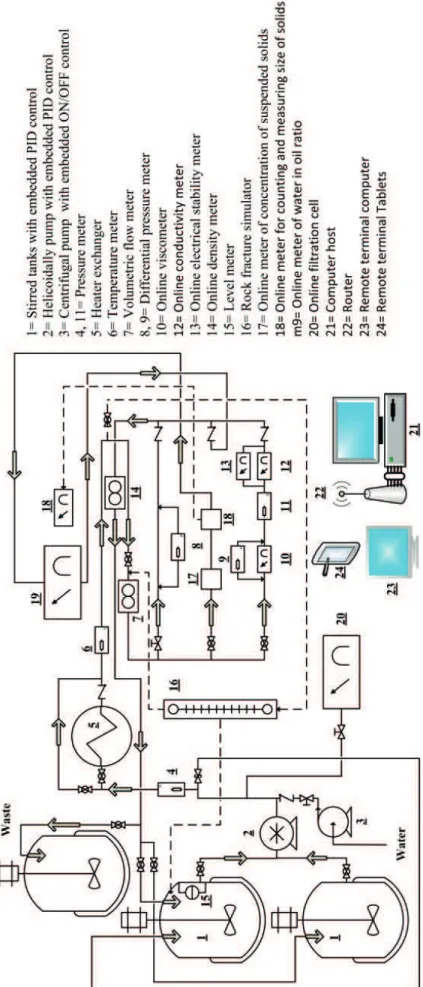
MATERIALS AND METHODS
Flow loop
The flow loop was built not only to develop the online
equipment, but also to make and produce the necessary
drilling fluids, whether oil-based or water-based. A brief
description of the apparatus is found in Fig. 1:
⸺ A500-liter tank coupled with a high power and speed mixer;
⸺ A3-hppositive displacement pump that drives the fluid
to the pipe lines;
⸺ A centrifugal pump in parallel to flush the system
during or after experiments;
⸺ A heat exchanger to heat up or cool down the fluid; ⸺ An online instrumentation to measure the desired fluid
properties and control operational conditions such
as flow rate, discharge pressure, pressure drop and
temperature;
⸺ To communicate with the equipment, hardware was used that was provided by National Instruments, along
with the software LabVIEW®, with which the
human-machine interface was constructed.
The online viscometers TT-100 and pipe can be
identified in Fig.1 by numbers 10 and 8, respectively.
TT-100 performs both shear rate and shear stress measurements. The pipe viscometer generates shear stress by the pressure drop measured in the instrument numbered 8, and the shear rate is calculated by the determination of the volumetric
flow rate, which is provided by the instrument numbered 7, a Coriolis mass flow meter.
Figur
e 1.
Viscometers
Couette viscometer, online and offline
The Couette measurement system is present in
TT-100, an online viscometer, and in FANN 35A, an offline
viscometer. Figure 2 illustrates the mechanical parts of
TT-100 (Brookfield manual, 1993).
Figure 2. Viscometer BROOKFIELD, model TT-100, original motor.
It can be observed in Fig. 2 that the gap for TT-100 is formed when the number 2 and 4 pieces are assembled. The original TT-100 comes with a DC motor with seven
fixed velocities, manually controlled.
The objective was not only to determine rheological behavior, but to control the equipment remotely. So the
original instrument was modified by replacing the DC
motor with an AC brushless servomotor. These types of motors are controlled with a special vector inverter device, which allows full access to several motor parameters, such as speed, torque, and spin control. The motor replacement also permits capturing the velocity of the motor (RPM) in real time.
As a result of the online configuration, the operating
principles of TT-100 are the same for any default Couette
viscometer – with the exception of the fluid renewal inside the measurement chamber. If the fluid changes its
rheological characteristics, TT-100 will report so as soon
as this fluid arrives in the gap.
The offline instrument evaluates the shear stresses at six different shear rates. The velocities of the outer cylinder
can be selected by manipulating simultaneously the speed selector along with the gear shift. The velocities are 3, 6, 100, 200, 300, and 600 RPM. The shear stresses, in each
motor velocity, are calculated from the values of deflected
angle, which can be read in the analogical display on top of the instrument.
Pipe viscometer
From experimental data of volumetric flow rate and
pressure drop, it was possible to estimate the shear rate and shear stress, respectively, using the mathematical models illustrated above. Figure 3 shows the constructed viscometer in greater detail.
Experimental design
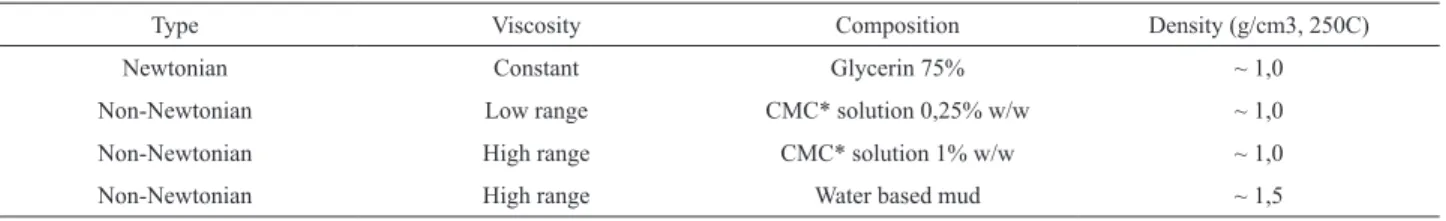
Fluids and experimental procedure
To investigate rheology online, the study used three
different fluids — one exhibiting Newtonian behavior and
two exhibiting Non-Newtonian behavior. The Newtonian
fluid was used to calibrate and validate the installed equipment. Because the fluid had fewer rheological
complexities, it was expected that all viscometers would provide similar data. After validation, a polymeric solution was used to evaluate the performance of each viscometer
against non-Newtonian fluid behavior. Finally, and of most
interest, all instruments were tested with a water-based
drilling fluid, typically used in drilling processes; the fluid has solids in suspension, in a medium concentration range (30 to 60 % in mass). Table 1 presents these fluids’
properties, such as composition and density.
Table 1. Evaluated fluids.
Type Viscosity Composition Density (g/cm3, 250C)
Newtonian Constant Glycerin 75% ~ 1,0
Non-Newtonian Low range CMC* solution 0,25% w/w ~ 1,0
Non-Newtonian High range CMC* solution 1% w/w ~ 1,0
Non-Newtonian High range Water based mud ~ 1,5
*CMC = Carboxyl Methyl Cellulose
The basic composition of the water-based mud was water, bentonite, barite, calcium carbonate, sodium hydroxide, xanthan gum, glutaraldehyde, and a rheological
modifier.
The experimental procedure consisted of acquiring, at
the same time, the rheological profile of the chosen fluid at the same temperature in all three instruments—TT-100,
FANN 35A, and pipe viscometer. Mathematical procedure
According to Billon (1996), many viscometers are
sold to be used with Non-Newtonian fluids containing mathematical procedures only valid for Newtonian fluids
to calculate apparent viscosity, shear rate and shear stress. The literature shows that the velocity gradients for
non-Newtonian fluids formed in a gap or during tube flow are not as parabolic as for Newtonian fluids. The smaller the value of n, the more non-linear is the profile formed by the
gradient velocity. Hence, the shear rate for non-Newtonian
fluids, regardless of the geometry of the flow, depends
directly on the behavior index and gap size. Ignoring these terms can lead to a miscalculation .As a result, an algorithm
was built in a LabVIEW® environment to solve Eq. (2). The algorithm applies a linear fit to the logarithm of the
income data of shear stress and motor speed. This algorithm can determine the slope of the line formed between those logarithms, which is n` (Eq. (5)). This calculation allows
the prompt determination of the dimensionless coefficient
(Eq. (3)) necessary to calculate the shear rate of
Ostwald-de-Waele fluids.
The linear fit is based on the iterative model (LabVIEW® instruction manual) represented by:
(
)
( )
1
2
0
1
,
ˆ
−
=
=
∑
N i i−
ii
residual
w y
y
N
where N is the number of data received,
i
w
is the ith element of weight,y
ˆ
i is the ith element of best linear fitand
y
i is the ith element of incoming data (dependentvariable). This study considered the weight equal to 1 and the tolerance equal to 0.0001.
For the offline viscometer, the linear fit was done using a native algorithm from the software ORIGIN®, which is
also based on the Least Square Method (LSM).
RESULTS AND DISCUSSION
Online rheology results
All evaluations were done at two different temperatures and in triplicate. The figures will only show the typical
average result at lower temperature. Complete data can be observed in the tables.
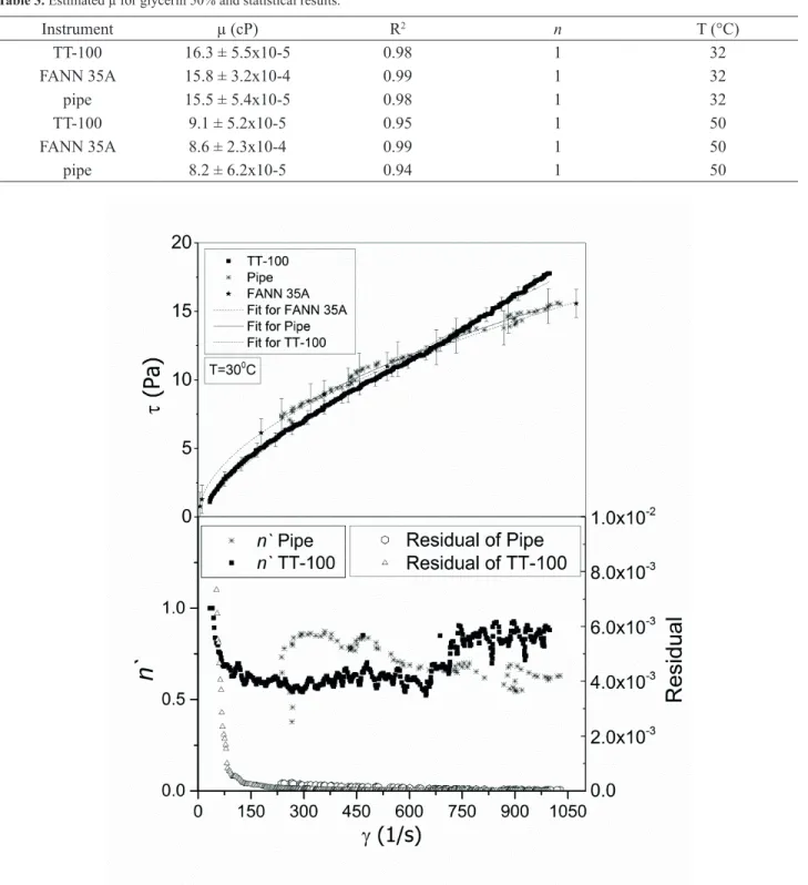
Figure 4 presents the rheological behavior and its statistics for glycerin. The statistical information can be
seen under the rheological profiles, respectively, according
to the horizontal aligned axis.
The behavior of the plotted shear stress versus shear rate was, as expected, a straight line, characteristic of a Newtonian behavior. TT-100 presented some divergence above 750 s-1. Besides that, all equipment presented similar
data.
The measurement range of the pipe viscometer was
limited by pump rotation and flow regime. Its inferior limit
Figure 4. Shear stress versus shear rate for glycerin and its statistical results.
was the minimum rotating speed of the pump, and the
superior limit was the maximum flow rate to maintain the
laminar regime.
One may also note the error bars, which represent the error propagation caused by sensor imprecision. Table 2 shows that all imprecisions accounted for this error propagation. The mathematical method used was the derivative one (Meyer, 1975).
In Fig. 4, it can be noted that the residual of TT-100was larger than that of the pipe viscometer at the beginning of operation, despite being smaller until the end of the experiment. Thereby it is possible to infer that
the incoming data (ln(τ) and ln(ω)) of TT-100 was more
accurate than that of the pipe viscometer. This is acceptable because the pump vector inverter is not as precise as the servomotor vector inverters. Despite the larger residual at
the beginning of the operation, TT-100 converged its slope faster than did the pipe viscometer.
To obtain the parameter µ of the Newtonian model,
another linear fit was applied, but now using data of shear rate and shear stress. This fit was done using the software ORIGIN®, which received the exported data from LabVIEW®.
The obtained results of viscosity (μ) and the performance of the fit (R² - correlation coefficient) are
presented in Table 3.
The results presented for n, in Table 3, permit the conclusion that the hypothesis of n = n` was acceptable.
To evaluate data for non-Newtonian fluid, a dilute
solution of CMC was fabricated, approximately 0.25% in
mass. Shown in Fig.5 is the data obtained for this fluid.
Table 2. Imprecisions considered for error propagation.
Instrument Imprecise measure dimension range TT-100 Deflected angle
Motor velocity
degree RPM
± 1% ± 1
FANN 35A Deflected angle degree ± 1
pipe Pressure
Flow rate
Pa m3/s
± 1% ± 1%
Table 3. Estimated µ for glycerin 50% and statistical results.
Instrument µ (cP) R2 n T (°C)
TT-100 16.3 ± 5.5x10⁻⁵ 0.98 1 32
FANN 35A 15.8 ± 3.2x10⁻⁴ 0.99 1 32
pipe 15.5 ± 5.4x10⁻⁵ 0.98 1 32
TT-100 9.1 ± 5.2x10⁻⁵ 0.95 1 50
FANN 35A 8.6 ± 2.3x10⁻⁴ 0.99 1 50
pipe 8.2 ± 6.2x10⁻⁵ 0.94 1 50
curve is characteristic of an Ostwald-de-Waele fluid, more
precisely a pseudo-plastic. To represent the curve a power law model was used. One may note once more the deviance for TT-100 rheological behavior after 750 s-1. Besides that, all equipment generated similar data.
The linear fit results presented are accurate. It may also
be noticed that the slope is more dynamical than it was for
Newtonian fluids. Usually rheological behavior measured online is subject to effects absent from batch offline systems
because, in the process, a perfect steady state would never be achieved (Himmelblau and Rigs, 2003). Evaluating the
results in Fig. 5, it can be understood that these effects are more pronounced with non-Newtonian fluids than with
Newtonian ones. The objective of having a dynamical n`
is to see how it impacts the final rheological profiles.
The n` for TT-100 was similar to that of FANN 35A, until it started to deviate to approximately0.87. The slope of the pipe viscometer did not maintain a constant value and diverged from TT-100. Therefore, two Couette viscometers were observed to generate similar slopes and a pipe viscometer to diverge from them.
Table 4 shows the results for the non-linear fit of
shear rate and shear stress, using the power law model to
represent the rheological profiles. There are present in the
table the parameters K and n, which belong to the power
law model, as well as n’avg and R². The parameter n’avg is the average value of n’ obtained during an entire online
rheological test. This average online parameter is directly
compared to the offline n’.
It can be seen in Table 4 that the values of the parameters K and n, for TT-100 viscometer, diverged from other instruments, probably because of its divergence at high shear rates (Fig. 5).
An increase of temperature decreases the values of the parameter K, which is expected as K is the number related
to the viscous aspect of the fluid. In addition, the behavior
index of FANN 35A and of the pipe viscometer remain
similar, but rises significantly for TT-100. This increase
in the TT-100 index happened because the slope did not diverge as it had in the previous experiment with low
temperature. Any changes in the rheological profile affect
directly the parameters estimated.
The divergences at a certain point for TT-100must be related to shear stress, which depends directly on the
torque sensor engineering. This behavior was investigated
to see if it was present during measurements in fluids with
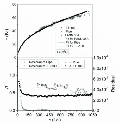
higher viscosities. The results of 1% CMC are presented in Fig. 6 and Table 5.
Figure 6 shows no more deviances at high shear rates for the TT-100 viscometer. It was thus concluded that the torque sensor of the studied instrument was more adequate and accurate for high-range viscosity measurements. This brings up one disadvantage of Couette systems; one should make preliminary tests to choose a torsion element
adequate to the viscosity range of interest (Brookfield
instruction manual, 1993 and Fann instruction manual, revision J 208878).
The power law parameters for this system can be seen in Table 5.
The parameter n` for the pipe viscometer and FANN
35A diverged from n, but for TT-100 was accurate. When
comparing data in Tables5 and 4 (the same temperature, but Table 4 was 0.25% CMC), it should also be noted that, as expected, an increase in the polymer concentration makes K rise (becoming more viscous) and n drop (becoming more non-Newtonian).
Making the fluid more non-Newtonian, with lower values of n, causes a pronouncement of some effects, such as gap size, border effects, and pressure drop effects. This
is experimental evidence which explains why n and n` diverged for FANN 35A and pipe viscometer. For FANN 35A, the gap is wider than the gap of TT-100; the wider the gap, the more pronounced is the associated error. For
the pipe viscometer, the more non-Newtonian the fluid, the more difficult it is to achieve the steady state of the flowing fluid, which makes it more difficult to measure volumetric flow rate.
An increase in temperature caused, as expected, a decrease in the parameter K. Also as expected, the
parameter n does not vary significantly. It was noted
that, for this high-range viscosity system, TT-100 was the instrument that provided the closest values of n` and n.
Once the effects of viscosity range and temperature
on the instruments were investigated, the next step was
to evaluate the effects of suspended solids in viscosity measurements during flow. Fig. 7 presents the rheological behavior ofa water-based drilling fluid with a density of
1.5 g/cm3.
Table 4. Estimated K and n for dilute 0.25% CMC and statistics results.
Instrument K n n’avg R
2 T(°C)
TT-100 0.10 ± 1.90x10⁻³ 0.75 ± 2.99x10⁻³ 0.69 0.99 30
FANN 35A 0.40 ± 2.70x10⁻² 0.52 ± 1.02x10⁻² 0.56 0.99 30
pipe 0.43 ± 1.80x10⁻² 0.52 ± 6.32x10⁻³ 0.58 0.99 30
TT-100 0.03 ± 3.35x10⁻⁴ 0.88 ± 1.62x10⁻³ 0.78 0.99 50
FANN 35A 0.24 ± 1.80x10⁻² 0.56 ± 1.15x10⁻² 0.52 0.99 50
Fig. 6. Shear stress versus shear rate for 1% CMC and its statistical results.
Table 5. Estimated K and n for 1% CMC and statistical results.
Instrument K n n’avg R
2 T (°C)
TT-100 2.72 ± 9.97x10⁻³ 0.46 ± 5.63x10⁻⁴ 0.44 0.99 33
FANN 35A 3.24 ± 0.52 0.44 ± 2.46x10⁻² 0.51 0.99 33
pipe 3.96 ± 0.13 0.40 ± 4.96x10⁻³ 0.58 0.98 33
TT-100 1.19 ± 6.85x10⁻³ 0.55 ± 8.76x10⁻⁴ 0.53 0.99 50
FANN 35A 1.66 ± 0.30 0.50 ± 2.76x10⁻² 0.62 0.99 50
pipe 2.08 ± 0.14 0.46 ± 1.00x10⁻² 0.54 0.96 50
After 750 s-1, the curve of TT-100 started to diverge, as
was observed previously with low-viscosity range fluids.
This was unexpected because the water-based mud is a
high-range viscosity fluid. Although the divergence pattern
is similar to the ones that occurred in previous experiments, the root of this divergence is distinct. The literature shows that the accuracy of Couette viscometers can be susceptible
to fluids with suspended solids—the more homogeneous the fluid the more accurate the measurement.
It is also known that the slippage effect can impact
viscometer readings when solids are suspended. The
slippage effect reduces measurement precision because
the velocity of the wall (spinning outer cylinder) and
the velocity of the fluid at the wall are not entirely equal
anymore. In summary, it was concluded that, when
evaluating fluids with suspended solids, there are at least two concomitant different effects on Couette instruments:
homogeneity and slippage.
For TT-100, the sample tended to be more homogeneous
than FANN 35A due to the flowing of the drilling fluid inside the measuring chamber. This flow rate, on the other hand, caused the slippage effect to be more pronounced. The β ratio (Eq. (4)) for TT-100 is 1.04 and for FANN 1.06. The narrower the gap, the more present the slippage effect,
Figure 7. Shear stress versus shear rate for a water based drilling fluid and its statistical results.
presented the highest values of shear stress and TT-100 the lowest (note that this impacts directly the value of the
K parameter). In addition, the slippage effect was more
pronounced at a lower shear rate, which explains why TT-100 tends, at high shear rates, to converge its rheological
behavior to FANN 35A.
The rheological parameters presented in Table 6 demonstrate that the slope for TT-100 was not steady at a common average point; this may be attributable to the
slippage effect.
Table 6. Estimated K and n for water-based drilling fluid and statistical results.
Instrument K n n’avg R
2 T (°C)
TT-100 1.85 ± 3.51x10⁻² 0.48 ± 2.90x10⁻³ 0.46 0.99 34
FANN 35A 4.20 ± 8.91x10⁻² 0.37 ± 3.28x10⁻³ 0.38 0.99 34
pipe 3.55 ± 0.26 0.38 ± 1.11x10⁻² 0.51 0.95 34
TT-100 1.34 ± 2.88x10⁻² 0.50 ± 3.29x10⁻³ 0.48 0.99 50
FANN 35A 3.15 ± 0.18 0.39 ± 9.07x10⁻³ 0.40 0.99 50
pipe 2.60 ± 0.26 0.40 ± 1.55x10⁻² 0.52 0.90 50
The best assumption for n` = n was found using TT-100
and FANN 35A viscometers. The online linear fit for
TT-100 at 50°C presented similar behavior compared to the previous one done at lower temperature.
Statistical analysis of the obtained results
the null hypothesis is: changing devices does not influence
the rheological parameters. To test this hypothesis, the STATISTICA software was used as computational tool.
The mathematical approach used was the “Kruskal-Wallis
ANOVA by Ranks”. Such method does not rely on data
distribution parameters (normal distribution for instance), therefore it is adequate for unknown small samples, such as presented here. The results obtained after performing the statistical test can be observed in Table 7.
Table 7. Results obtained from Kruskal-Wallis statistical test.
Variable Coded variable Significance (p-level) Result over null hypothesis
K n
Device TT100 / FANN 0.6907 0.5020 Accept Accept
Fluid G/C1/C2/ WBM* 0.002 0.002 Reject Reject
* G – Glycerin, C1 – CMC at 0.25%, C2 – CMC at 1%, WBM – Water Based Mud
A 95% confidence interval was chosen; p-level limit
was automatically created at 0.05. In Table 7, it can be seen that this parameter was 0.002 when computing the
influence of the fluid over the parameters K and n. This
means a probability of 99.998% that the null hypothesis is wrong, or a probability of 0.002% that the null hypothesis is right. Therefore, every p-level below 0.05 should reject the null hypothesis, as the opposite is true. In an overall analysis, considering still Table 7, the nature of the
fluid presented statistical influence over the rheological
parameters. On the other hand, changing devices did not. In conclusion, it can be inferred that the divergences found
in the rheological parameters during the usage of different
devices are not statistically relevant.
Investigation of the measured rheology on friction loss determination.
One of the major tasks during the drilling of petroleum wells is to determine the friction loss for pressure control.
The rheological parameters influence this calculation directly. Thus to evaluate the impact of the different
rheological behaviors obtained on the calculation of friction loss, a case study was conducted. Experimental data of pressure loss were collected for water-based mud and
then compared with the calculated ones. The operational
condition was at 50˚C, in a straight pipe line with 30-cm length, 11.5-mm diameter, made of CPVC, with a flow rate
of0.26 m3/h (laminar regime). To calculate the pressure loss, the following was used,
( )
2 2,
2
10
ρ
=
dL
v
P
f
D
where( )
64
,
=
PLf
Re
and( )
1.
8
3
1
4
ρ
−=
+
PL n n
Dv
Re
v
n
K
D
n
with
P
d being the calculated pressure drop,L
the lengthof the pipe,
D
the internal diameter,v
the averagevelocity of the fluid,
ρ
the specific mass of the fluid, andK
and n the power law parameters provided by the onlineand offline instruments. The results are shown in Table 8.
Table 8. Estimated pressure drop in a straight pipe line for a water-based drilling fluid, at 50oC, laminar regime.
Instrument K n Pd(mBar)
calculated
Pd(mBar)
experimental Error
TT-100 1.34 0.50 34.39
34.25
0.41%
FANN 35A 3.15 0.39 41.67 17.81%
pipe 2.60 0.40 36.54 6.27%
It can be seen that the viscometer that provided the smallest error (calculated value – experimental value) was TT-100, even with its deviance after 750 s-1.The pipe viscometer provided a small error, and FANN 35A the highest one, although the steadiest curve. These
results reinforce the notion that not always the best fit of
rheological data generates the best prediction of pressure loss. In this case, the best prediction of pressure drop was given by the TT-100 rheological measurement.
(10)
(11)
CONCLUSIONS
Within a fluid loop, this work developed and installed two online viscometers to measure drilling fluid rheological
behavior simulating a well-drilling operation. One was
a modified Couette viscometer and the other a standard
pipe viscometer. For validation, the study compared the performance of both instruments with FANN 35A,
which is an offline viscometer that the petroleum industry
commonly uses as benchmark.
For a Newtonian fluid, agreement was found in all
instruments between data for viscosity, proving that the devices were properly calibrated and installed. For
non-Newtonian fluids, there were divergences in the
power-law parameters provided by each instrument, both for
drilling fluid (with suspended solids) and polymeric
solution. Similar results were observed in the previously cited literature. These divergences were investigated and the probable main causes were found to be the following:
effects of homogeneity, slipperiness, and interactions in the fluid/gap interfaces. In addition, a case study was carried
out that demonstrated that these divergences were not
significant if the parameters were used for pressure drop
calculations. As an overall conclusion, the methodology proposed can be used to obtain online measurements
of drilling fluid rheological behavior as well as online
prediction of friction loss. In consequence, this paper
contributes significantly to overcome the initial steps
toward a fully automated drilling operation.
ACKNOWLEDGEMENTS
This work is developed by a partnership between PPGEQ/UFRRJ and CENPES/PETROBRÁS under the thematic network of research and engineering. The authors
wish to acknowledge CENPES for their financial and
service support.
NOMENCLATURE
Symbol Description Unit (SI)
τ Shear stress Pa.s
k Elastic constant N.m/degree K Consistency index (kg/m)*(1/s)2-n
H Height of the inner
cylinder m
θ Deflected angle Degree
γ
Shear rate 1/s
Ø
Correction Factor Dimensionless r2 Outer cylinder radius mr1 Inner cylinder radius m
ω Angular velocity rad/s
β Radius ratio Dimensionless
n Behavior index Dimensionless
n’ Pseudo behavior
index Dimensionless P Pressure Pa
z Orientation index
Cartesian) -x Orientation index
(Cartesian) -r Tube or pipe position
on radius m
L Tube or pipe length m
v Velocity of the fluid m/s
v
Average velocity ofthe fluid m/s
R Tube or pipe radius m hd Friction loss in a straight pipe line m
Q Volumetric flow rate m3/s
f Friction factor Dimensionless H Height of the inner
cylinder m
D Tube or pipe diameter m g Gravity m/s2
RePL Reynolds for Power
Law fluids Dimensionless
wi ith element of the array
or matrix weight Dimensionless
ˆ
iy
ith element of the array
or matrix of best fit According to data
yi ith element of the array
or matrix of observed
values According to data N Size of the array
or matrix Dimensionless
REFERENCES
Apaleke, A. S, Al-Majed, A. and Hossain, M. E., Drilling fluid:
state of the art and future trend. North Africa technical conference and exhibition, Cairo, Egypt. SPE 149555 (2012).
Barnes, H. A., A Handbook of Elementary Rheology, Institute
of Non-Newtonian Fluid Mechanics, University of Wales
(2000).
Billon, H.H., Shear Rate Determination in a Concentric Cylinder Viscometer, DSTO Aeronautical and Maritime Research Laboratory, PO Box 4331, Melbourne Victoria 3001. Publication track AR-009-701, DSTO-GD-0093 (1996).
Bird, R.B, Steward, W.E. and Lightfoot, E.N., Transport
Phenomena. Second Edition. Chemical Engineering
Department. University of Wisconsin-Madison (2001). Brookfield viscometers, Instruction Manuals and Guides (1993).
Drilling Conference and Exhibition, Abu Dhabi, UAE.SPE 137999 (2010).
Caenn, R. and Chillingar, G.V., Drilling fluids: State of the Art.
Journal of Petroleum Science and Engineering. 14, 221–230 (1996).
Craft, Holden and Graves, Well Design: Drilling and Production. Prentice – Hall, Inc. Englewood Cliffs, New Jersey (1962).
Carlsen, L. A. and Nygaard, G., Utilizing Instrumented Stand Pipe for Monitoring Drilling Fluid Dynamics for Improving Automated Drilling Operations. Proceedings of the 2012
IFAC Workshop on Automatic Control in Offshore Oil
and Gas Production, Norwegian University of Science and Technology, Trondheim, Norway (2012).
FANN instruments, revision J 208878. Model 35 Viscometer Instruction Manual.
Gandelman, R. A., Martins, A. L., Teixeira, G. T., Aragão, A. F. L., Neto, R. M. C., Lins, D. G. M., Lenz, C., Guilardi, P. and Mari, A., Real Time Drilling Data Diagnosis Implemented In
Deepwater Wells - A Reality,
OTC-24275-MSOTC-24275-MS, Rio de Janeiro, October 29th to 31th, Brazil (2013).
Himmelblau, D.M. and Riggs, J. B., Basic Principles and Calculations in Chemical Engineering: International Edition, 7/E. Pearson Education. University of Texas, Austin (2013).
LabView® instruction manual and online Help(2011).
Macosko, C. W., Rheology: Principles, Measurement and Applications. Wiley-VCH – Inc. Originally publish as ISBN
1-56081-579-5 (1994).
Meyer, S. L., Data Analysis for Scientists and Engineers, Wiley
ISBN 0-471-59995-6 (1975).
Morrison, F. A., Understanding Rheology, Oxford University Press, Inc. ISBN 0-19-514166-0 (2001).
Oort, E. V. and Brady, K., Case-Based Reasoning System Predicts
Twist-off in Louisiana Well Based on Mideast Analog.
Special Focus – Drilling Technology (2011).
Paraíso, E. C. H., Study of cement slurries flow in circular and
concentric annular ducts, Thesis, Federal Rural University of Rio de Janeiro (2011).
Rondon, J., Barrufet, M. A. and Falcone, G., A novel downhole
sensor to determine fluid viscosity. Flow Measurement and
Instrumentation, 23, 9-18(2012).
Saasen, A., Omland, T. H., Ekrene, S., Breviere, J., Villard, E., Kaageson-Loe, N., Tehrani, A., Cameron, J., Freeman, M., Growcock, F., Patrick, A., Stock, T., Swaco, M.I., Jørgensen, T., Reinholt, F., Scholz, N., Amundsen, H. E. F., Steel,e A., and Meeten, G.,Automatic Measurement of Drilling Fluid and Drill Cuttings Properties. IADC/SPE Drilling Conference (2009).SPE Drilling &Completion, 24(04), 611-625 (2009).
Shaughnessy, J., Daugherty, W., Graff, R. and Durkee, T., More
Ultra-Deepwater Drilling Problems. SPE/IADC Drilling Conference, ID: 105792-MS. ISBN 978-1-55563-158-1 (2007).
Vajargah., K. andvan Oort., E., Determination of drilling fluid