Article
Printed in Brazil - ©2017 Sociedade Brasileira de Química 0103 - 5053 $6.00+0.00
*e-mail: [email protected]
Multivariate Calibration to Determine Phorbol Esters in Seeds of
Jatropha curcas
L.
Using Near Infrared and Ultraviolet Spectroscopies
Jussara V. Roque,a Luiz A. S. Diasb and Reinaldo F. Teófilo*,a
aDepartamento de Química and bDepartamento de Fitotecnia, Universidade Federal de Viçosa,
36570-900 Viçosa-MG, Brazil
The building of partial least squares (PLS) regression models using near infrared (NIR) and ultraviolet (UV) spectroscopies to estimate the concentrations of phorbol esters (PEs) in Jatropha curcas L. is presented. The models were built using two algorithms for variable selection, ordered predictors selection (OPS) and genetic algorithm (GA). Chromatographic analyses were performed to determine the concentrations of PEs. Spectral data were obtained from seeds and oil extract. The results of PLS models were performed by analyzing statistical parameters of quality such as root mean square error of prediction (RMSEP) and correlation coefficient of external predictions (Rp). The parameters obtained for NIR-PLS and UV-PLS models with OPS
were respectively: RMSEP 0.48 and 0.22 mg g-1 and R
p 0.49 and 0.96. For GA were obtained,
respectively: RMSEP 0.52 and 0.28 mg g-1 and R
p 0.12 and 0.95. The models built from seeds
and oil extracts can be used respectively for screening and to accurately predict the PEs content. The OPS method provided simpler and more predictive models compared to those obtained by the selection of variables using the GA. Thus, the UV-PLS-OPS model can be used as an alternative method to quantification of PEs.
Keywords: phorbol esters, Jatropha curcas L., multivariate calibration, near infrared, ultraviolet spectroscopy
Introduction
Currently, fossil fuels are the major energy source used by mankind. However, this has resulted in an increase in anthropogenic greenhouse gas emissions in the atmosphere that contributes to the increase in average temperature of the earth and complex changes in climate.1 Fossil fuels,
such as gasoline and natural gas, are limited and will be insufficient for the world’s energy demands in the near future. Biofuels, such as biodiesel, are a strategy that combines energy security and sustainability.2,3
Biodiesel derived from vegetable seed oils is an alternative to diesel fuel as a renewable and environmentally clean source of energy. This fuel has been produced from a variety of vegetable sources, such as soybean,4
sunflower,5 palm oil6 and physic nut.7,8 In this context,
Jatropha curcas L., also known as physic nut, stands out as one of the most promising non-edible oil seeds for the production of biofuel.9,10
J. curcas is a small tree or large shrub, which belongs to the Euphorbiaceae family and has a life expectancy
of up to 50 years.11 Mexico is the center of origin and
domestication of J. curcas,8,12 but this plant spontaneously
grows in different regions of Brazil and around the world, including Africa, India, Southeast Asia and China.13 The
J. curcas seed contains approximately 31% oil (ranging from 16 to 45%),14 presenting a composition of fatty acids
that provide biodiesel with excellent properties.15 The press
cake remaining after oil extraction is rich in proteins and has potential for use in animal feed, adding value to the productive chain of biodiesel.16,17 However, the press cake
contains toxic compounds, such as phorbol esters (PEs),18
which limit its use for this purpose.19 Fortunately, there are
reports of the existence of germplasm free of these toxic compounds.20
PEs were first identified in 1984 by Adolf et al.21 Six
High-performance liquid chromatography with a diode array detector (HPLC-DAD) is broadly used to determine PEs. This technique presents good separation and low limits of detection.23,24 Nevertheless, these analyses are
time-consuming, laborious, expensive, environmentally harmful and destructive, which can, in some cases, preclude the evaluation and selection of genotypes for the development of cultivars. Alternatively, fast, environmentally friendly and non-destructive analyses are possible using spectroscopic techniques and multivariate calibration.25
Near infrared spectroscopy (NIR) has been widely used to measure the quality of agricultural and food products.26 This non-invasive spectroscopic technique
can rapidly provide information on physical and chemical samples. Baye et al.27 used NIR to predict seed corn
compositions. Choung et al.28 used NIR for determining
the protein and oil contents of soybean. Helgerud et al.29
used NIR for online prediction of dry matter content in whole unpeeled potatoes.
Another spectroscopic technique, ultraviolet (UV), combined with multivariate calibration has become quite popular for quantification of interesting species. In the literature, several prediction models using this combination can be found, such as quantification of tannins,30 determination of wine acidity31 and
simultaneous determination of caffeine and paracetamol in pharmaceuticals.32 As UV spectroscopy is based on
electronic transitions, in most cases, the technique has the ability to detect low concentrations of the analyte of interest. In contrast, NIR spectroscopy is based on vibrations and therefore has limitations at high limits of detection, larger than mg L-1.
There are several multivariate regression methods. Among them, we highlight regression by partial least squares (PLS), recognized as the most widely used method for building first order calibration models from chemical source data. This method does not require accurate knowledge of all the components present in the samples and it is able to perform prediction of an analyte of interest even in the presence of interference, as long as the interferents are also present in the model building.33 PLS
can be used in highly correlated noise and experimental data, allowing simultaneous modeling and prediction of more than one analyte, i.e., a matrix Y.34,35 Firstly, the
model is built and validated. After that, it can be used for predictions of unknown samples, without the need to carry out a reference analysis.
Thus, the aim of this work was to build multivariate calibration models for analysis of PEs using spectroscopic and chemometric methods. NIR and UV spectra were obtained from J. curcas seeds and oil extract. The
HPLC-DAD technique was used as the reference method to determine the PEs.
Experimental
Materials
The J. curcas samples used in this work belong to a germplasm active bank (GAB) and a progeny test (PT). A total of 77 samples of the GAB were used, being 74 taken from different regions of Brazil and 3 from Cambodia. A total of 121 samples were obtained from the PT. Both the GAB and PT were carried out in 2008 at the Universidade Federal de Viçosa (UFV). Based on this set (GAB plus PT, a total of 198 samples), 100 samples were selected using the principal component analysis (PCA). Each sample comprises a set of seeds with shells.
Phorbol-12-myristate-13-acetate (PMA) was obtained from Sigma-Aldrich (≥ 99%; TLC). The solvents, methanol (CH3OH) and acetonitrile (CH3CN), used in this study were
of HPLC grade (J.T. Baker; 99.95%), while formic acid (HCOOH) was of analytical grade (Panreac; ≥ 98.0%).
J. curcas sample preparation
The oil was extracted from samples manually pressed with the aid of a mechanical press. Approximately 20 mL of oil was obtained, placed in amber glass bottles and stored under refrigeration (−20 °C).
PEs extraction was carried out by means of adjustments of the optimized methodology found in the literature.36
PEs were mechanically extracted from J. curcas oil with methanol (1:2 m/v) using a magnetic stirrer at 60°C for 5 min. The resulting mixture was gravity separated and the upper methanol layer was collected. The described process was repeated three times to quantitatively extract the PEs. Finally, the methanol extracts collected were evaporated and the residue was stored under refrigeration at −20 °C.
PEs analysis
PEs were determined in duplicate. Briefly, the stored residue was re-dissolved in 4 mL of methanol and filtrated (nylon filter with 45 µm pore size and 25 mm diameter) to injection vials. Samples of 20 µL were analyzed by HPLC.
The HPLC used for method development and validation was a Shimadzu® 20AT prominence separations module
interfaced with a Shimadzu® SPD-M20A prominence
Kinetex® (Phenomenex, 100 × 4.6 mm, 2.6 µm) was used.
A head column containing the same material was used to protect the column.
A central composite design (CCD) was performed to optimize the mobile phase composition in the chromatographic method to obtain the best peak separation and smallest analysis time. Thus, the acetonitrile percentage (CH3CN% 79-86%) and formic acid concentration
(HCOOH% 0.45-0.75% v/v in water) were evaluated. The response variable, y, was obtained by the combination of chromatographic parameters to obtain the desired response (DR), as shown in equation 1.
(1)
where rtF is the retention time of the last peak and np is the number of peaks that appear in retention time of PEs, not necessary separated. The quantification of the PEs is done by sum of the total area of all peaks that appear in the retention time of PEs. Thus, complete separation of the peaks is not necessary.
It is desirable to find the lowest rtF because this corresponds to a shorter run time and np = 5 is considered optimal since it indicates the separation of the five PEs present in J. curcas (the two Jatropha factors epimers appear in the same peak). Thus, the DR considered optimal, obtained by the equation, is the lowest possible. All calculations were performed using spreadsheets according to Teófilo and Ferreira.37
The mobile phase was further degassed and filtered through nylon membrane filters (0.45 µm). The column was eluted using an isocratic gradient at a flow rate of 1 mL min-1. The column temperature was maintained at
30 °C and the detection wavelength was 280 nm. Methanol was used as the diluent during the standard and test sample preparation.
PMA was used as an external standard and the area of the PEs peaks was summed and converted to PMA equivalent (mg mL-1) by taking its peak area and concentration.23,36
Seven calibration solutions containing the PMA standard in the range 0.05 to 2.80 mg mL-1 were used to build the
inverse linear univariate regression.
In order to identify the chromatographic peaks, the spectra were compared to those in the literature.38,39
Spectral analysis
NIR spectra were measured by a Fourier transform near infrared (FT-NIR) spectrometer (Thermo Scientific Antaris II) controlled with TQ Analysis software. The FT-NIR spectrometer was operated in an integrating sphere
diffuse reflectance module. Seed scans were the average result of 32 scans measured with 8 cm-1 resolutions over the
wavenumber range 10000-4000 cm-1. These spectra were
obtained in reflectance mode as log (1/R), where R is the collected reflectance. Each intact seed was directly centered on the instrument window, without any sample preparation, and scanned on both sides. Each side was measured three times and the averaged spectrum of the two sides of each seed was used for the final analysis.
UV spectra were obtained by an Ocean Optics spectrometer (USB4000-UV-VIS) with the Spectra Suite Spectroscopy Operating software. Spectra were measured in duplicate using a quartz cuvette with a 10 mm optical path. Oil extract scans were the average result of 10 scans measured with 0.166 nm resolutions over the range 210-350 nm. These spectra were obtained in transmittance mode, where absorbance is collected. Oil extract was prepared from the dilution of the solution used in the PEs analysis in HPLC. The diluted solution was prepared in 2 mL of methanol with the addition of 600 µL of the stored oil extract.
Multivariate calibration models
Spectra were exported from each instrument software and imported by Matlab 2016a (Math Works, Natick, USA). An inverse regression model (y = Xb) was built using the PLS.33,34,40 The algorithms for the data import, the building
and the validation models were written in our laboratory in a function .m to Matlab. All calculations were performed in Matlab.
The data matrices used as input for PLS regression are denoted by XNIR and XUV, where each row in XNIR and XUV corresponds to a given spectrum from the seeds in the NIR spectra and the oil extract in the UV spectra, respectively. The y vector used to build the regression is related to values experimentally obtained through the chemical analysis by the HPLC method. The variables XNIR, XUV and y have been pre-processed using centering in all calculations. Transformations were carried out on the rows of the matrix
XNIR and XUV in order to find the best model for prediction. The transformations tested were first and second derivatives and the multiplicative scatter correction (MSC).
Regression models were evaluated on calibration and external validation steps by calculating the number of outliers excluded, root mean square error of calibration (RMSEC), correlation coefficient of calibration (Rc)
root mean square error of cross-validation (RMSECV), correlation coefficient of cross-validation (Rcv), root mean
The original data set was then split into calibration and validation sets using the Kennard-Stone41 algorithm
after outlier removal. According to ASTM E1655,42 for
regression models with five or less latent variables (h), the validation set should have at least 20 samples. When h is higher than five, the set must have approximately four times the number of model latent variables.40 Thus, a validation
set was used for external prediction and the remaining samples were used in the calibration set. The RMSE was calculated according to equation 2 and the correlation coefficient (R) is given by equation 3.
(2)
(3)
where y is the experimental value, ŷ and ŷ are the scalar and vector of the estimated values, respectively, ȳ is a scalar of mean values in y and Im is the number of samples.
The number of h in the model was determined by internal validation (cross validation, CV) applying the randomic removal of three samples. In cross validation, when Im is
the number of samples of calibration set (training), the error and correlation coefficients are named RMSECV and Rcv, respectively. When Im is the number of predicting
samples (P), the error and correlation coefficients are named RMSEP and Rp, respectively.
Bias is defined as the difference between the value measured and a reference value, it is a measure of systematic errors in the model, calculated with just the validation samples. This parameter can be obtained by equation 5, at which yi is the experimental value , ŷi is the
estimated value, Im is the number of predictions.
(4)
The standard deviation of validation (SDV) calculated by equation 5 is used for evaluating the statistical significance of the bias using a t-test(equation 6), where nv is the degrees of freedom.
(5)
(6)
Additionally, methods of variable selection are applied to select regions that present relevant information and are better correlated with the concentration of PEs in J. curcas samples. In this work, two methods were used, ordered predictors selection (OPS)43 and genetic
algorithm (GA).44
The OPS method is based in obtaining an informative vector that contains information about the location of the best response variables for prediction. The original response variables (X matrix columns) are differentiated according to the corresponding absolute values of the informative vector elements. The differentiated variables are sorting in descending order. Multivariate regression models are built and evaluated using cross validation. An initial subset of variables (window) is selected to build and evaluate the first model. Then, this matrix is expanded by the addition of a fixed number of variables (increment) and a new model is built and evaluated. New increments are added until all or some percentage of variables are considered. Quality parameters of the models are obtained for every evaluation and stored for future comparison. In the last step, the evaluated variable sets (initial window and its extensions) are compared using the quality parameters calculated during validations.43 The calculations were
performed using OPS_Toolbox.45
In the OPS method, when using the information vector, special attention should be given to the number of latent variables, h, to be used to obtain this vector. Firstly, it is determined the number of latent variables, h = hMod, to construct and validate the model. But maybe hMod cannot generate a informative vector sufficiently informative for variable selection. To find the best informative vector, a study was then performed on the full data set by increasing the number of components in the model, starting from h = hMod and carrying out the variable selection using the OPS algorithm. By varying the h value, different informative vectors are generated, from which the best component number (h = hOPS) is selected. Therefore, two optimum numbers of components are employed in this work, one representing the component number for model building (hMod) and the other representing the component number employed to generate the best informative vector in OPS method (hOPS).43
ones indicates if variables (individuals) should be included (1) or not (0). The parameters previously optimized and introduced into the algorithm were a population of 54, a maximum generation of 300, a mutation rate of 0.008, a window width of 1, convergence of 80, 50 terms included at initiation, cross-over rule of 2, number of subsets to divide data into for cross-validation of 3, cross-validation iteration of 1 and replicate runs to perform of 3.
Figures of merit
Among the most important figures of merit, sensitivity, selectivity and limit of detection (LOD) are related to the concept of net analyte signal (NAS). This concept plays an important role in the calculation of figures of merit for characterizing a calibration model. Thus, NAS vector has been defined as the part of a mixture spectrum that is unique for the analyte of interest, i.e., it is orthogonal to the spectrum of interferences.46,47
The sensitivity (SEN) is the slope of the calibration curve. Multivariate models are built as inverse regression, therefore, the SEN, according to equation 7, is the inverse of the regression coefficients estimated by PLS.48
(7)
where ||b|| is the Euclidean norm of regression coefficients vector estimated by PLS regression.
The analytical sensitivity,γ, is the ratio between the sensitivity and standard deviation of reference signal (∂x)
estimated by the standard deviation of the NAS about the reference signal spectra,49,50 as given in equation 8.
(8)
The inverse of this parameter (γ-1) allows us to establish
the lowest difference of concentration between samples, which can be distinguished by the method.
Selectivity (SEL) is the model’s ability to determine particular analytes in mixtures or matrices without interference from other components or simply a measurement of the amount of the signal used in the determination. In multivariate calibration, the value of SEL measured is generally low. Nonetheless, the model might be able to estimate the concentration of the analyte in the presence of interferents. This parameter is calculated according to equation 9,46,51 at which nas
k,i is the scalar
value for sample i and xk,i is the instrumental response
vector for sample i.
(9)
The LOD is the smallest amount of analyte that can be detected.52,53 The LOD calculation in multivariate
calibration is the most questioned and is not very well defined. Thus, several works have proposed calculations more precise for this parameter.54,55 In this work, the method
proposed by Ortiz et al.55 was used, which evaluates the
false positive and false negative hypothesis. This method is based on the extrapolation of a regression equation, obtained by the measured and predicted values, until a zero value of concentration. The LOD expression is calculated by equation 10.55,56
(10)
where the term is an estimate of the error in the intercept and the factor ∆(α, β) depends on the probability
α (type I error) and β (type error II) and on the number of degrees of freedom.
Results and Discussion
Central composite design
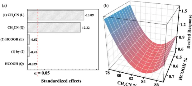
Statistical analysis by mean square residual error and the significance level (α) at 0.05 indicates that only CH3CN%
is significant, as shown by the Pareto chart (Figure 1a). The linear regression coefficient for CH3CN% was negative,
indicating that increasing the percentage decreases the last peak retention time to give the desired response, i.e., lower DR (equation 1). Moreover, the significant quadratic coefficient for CH3CN% indicated the DR decreases
quadratically as the CH3CN% increases until 84%, while DR
increases quadratically with a CH3CN% more than 84%, as
shown in the response surface (Figure 1b). Both CH3CN%
coefficients were significant (p = 1.20 and 1.70 × 10⁻⁵,
linear and quadratic coefficients, respectively). However, HCOOH% did not significantly influence the DR (p = 0.62 and 0.97, linear and quadratic coefficients, respectively) and the interaction between CH3CN% and HCOOH% was also
not significant (p = 0.65).
Analysis of variance (ANOVA) shows that the regression model is significant (p = 3.62 × 10⁻⁵) and with a
non-significant lack-of-fit (p = 0.19). These results suggest that the fitted response model can be applied to determine the optimum mobile phase composition.
was not significant, and it was obtained the lowest DR across of the studied range. Therefore, the optimal mobile phase composition chosen was 82.5% CH3CN and the
HCOOH concentration was 0.60% (v/v). This mixture provided a good chromatographic separation of J. curcas
samples in a run time of 4.5 min.
PEs quantification and identification
PEs peaks (five) appeared between 2.5 and 4.5 min (Figure 2a) and were monitored at 280 nm. The area of each peak was obtained and these results were expressed as equivalents of PMA, which was used as a marker and appeared between 5.2 and 5.8 min.
The inverse regression equation obtained for quantification of PEs was [PE] = 4.482 × 10⁻⁷SA − 0.01897,
where SA is the sum of the chromatographic peaks areas and [PE] is the PEs concentration. The linearity, expressed by R, was equal to 0.9968. This value indicates high model linearity within the concentration range studied.
The precision was evaluated as a measure of reproducibility of the entire analytical method, it was expressed by the relative standard deviation (RSD) calculated by the ratio of the standard deviation and the average of the chromatographic peaks areas of five replicates. The RSD value of 11.16% obtained may be considered appropriate and acceptable because of the complexity of the samples.
The LOD and limit of quantification (LOQ) (i.e., the lowest concentration of an analyte in a sample that can be determined with acceptable precision and accuracy) were determined by calculating a signal to noise ratio of 3:1 (LOD) and 10:1 (LOQ) between the standard deviation value regarding the chromatographic signal of seven blank
injections (CH3OH) and the slope of the calibration curve.
LOD and LOQ found were 0.0051 and 0.0171 mg mL-1,
respectively.
The seed PEs concentration in mg g-1 was obtained
according to oil content for each sample (access and progenies) and it ranged from 0.206 to 3.406 mg g-1.
Several concentrations ranges have been reported for PEs depending on the region where the samples were obtained. In Malaysia, the concentration of 3.0 ± 0.16 mg g-1 was
reported in 2001.57 Makkar et al.58 found concentrations
between 0.87 and 3.32 mg g-1 in countries of West and
East Africa, North and Central America and Asia. Another study of Makkar et al.18 evaluated four varieties of J. curcas
originated in Cape Verde, Nicaragua, Nigeria and Mexico. Concentrations of 2.17, 2.30 and 2.70 mg g-1 have been
reported for samples from Nicaragua, Nigeria and Cape Verde, respectively. The Mexican variety was described as non-toxic with only 0.11 mg g-1. Recently, concentrations
between 0.00 to 10.3 mg g-1 were described containing
samples from a wide variety of geographic regions around the world.25 Ferrari et al.59 evaluated J. curcas seeds from
different regions of Brazil and the PEs concentrations found ranged from 1.41 to 8.97 mg g-1.
In order to confirm the presence of PEs, individual
J. curcas PEs peaks, separated by the HPLC, were evaluated for absorption spectra. The absorption spectra of five peaks were similar to those reported in the literature.23,38,39 The
spectra of each of Jatropha factor (C1-C6) are shown in Figures 2b-2f.
Multivariate calibration models
In this section, we describe the model obtained using NIR spectra of the seeds, which presented results for
screening concentrations of PEs with quick decision-making for use in genetic breeding programs. The model built with oil extract UV spectra will also be presented, which showed satisfactory results and conditions to predict PEs concentrations with high accuracy. In addition, several models were built using the NIR and UV spectra of the kernel and oil of J. curcas. However, these models were not satisfactory and the results are not shown.
NIR spectra of J. curcas seed
Before building the model, transformations were carried out in order to find the best model for prediction. Thus, based on RMSECV values, it was observed that all transformations tested increased the error, and in this way, the spectra were just centered. Statistical parameters calculated for built models are shown in Table 1. The correlation coefficients (Rc, Rcv and Rp) are considerably
higher for the NIR-PLS-OPS model. Thus, the model that used selected variables was considered more efficient and robust. NIR spectra of J. curcas seeds with the variables selected by OPS are shown in Figure 3a.
In Figure 3c, the measured versus predicted values from the NIR-PLS-OPS model show that although the model presents high prediction errors, there is a linear fit between these values.
The NIR-PLS-OPS model was evaluated in order to verify if there was a correlation by chance. Hence, the vector
y was randomized and models were built with this random
y. Thus, the correlation parameters of these models were evaluated for both, random and measured y values. If these parameters of measured y distance themselves from the correlation values of the random y, it is an indication that the model did not occur by chance. Figure 3e shows that the NIR-PLS-OPS model (true model) is separated from the other models, so, the true model was not obtained by chance.
Montes et al.25 presented multivariate calibration
models to predict several J. curcas properties, including PEs concentrations. The authors showed that PEs could be determined by NIRS for qualitative classification purposes by excluding samples with low concentrations (< 0.1 mg g-1). The NIR-PLS-OPS model obtained in
our study can also be used for qualitative classification purposes. However, the model presented in this work was
Table 1. Statistical parameters of NIR-PLS and UV-PLS models with full variables and selected variables by OPS and GA methods, and figures of merit for UV-PLS models
NIR-PLS model UV-PLS model
Full OPS GA Full OPS GA
h 4 5 (hOPS = 19) 4 8 8 (hOPS = 11) 8
nVarsa 1556 130 85 656 85 85
RMSEC / (mg g-1) 0.4242 0.3131 0.4016 0.1914 0.1881 0.1913
Rc 0.2957 0.7528 0.3518 0.9491 0.9508 0.9381
RMSECV / (mg g-1) 0.4408 0.4335 0.4121 0.3190 0.2747 0.2499
Rcv 0.1776 0.4409 0.2861 0.8570 0.8947 0.8929
RMSEP / (mg g-1) 0.4441 0.4858 0.5271 0.2780 0.2273 0.2821
Rp 0.0076 0.4976 0.1276 0.9326 0.9602 0.9526
Bias 0.0026 0.0001 0.0003 0.0041 -0.0061 0.0014
γ-1 / (mg g-1) NCb NCb NCb 0.0404 0.0821 0.1007
SEL NCb NCb NCb 0.1081 0.1664 0.1714
LOD / (mg g-1) NCb NCb NCb 0.2895 0.2666 0.2607
aNumber of variables; bnot calculated. h: latent variables; RMSEC: root mean square error of calibration; R
c: correlation coefficient of calibration; RMSECV:
root mean square error of cross-validation; Rcv: correlation coefficient of cross-validation; RMSEP: root mean square error of prediction; Rp: correlation
coefficient of external prediction; SEL: selectivity; LOD: limit of detection.
Figure 3. (a) NIR and (b) UV spectra of Jatropha curcas L. seeds (XNIR) and oil extract (XUV), respectively, with the variables selected by OPS algorithm (vertical lines); (c) NIR-PLS-OPS model and (d) UV-PLS-OPS model: measured versus predicted values of PEs contents for the calibration () and prediction () sets; (e) NIR-PLS-OPS model () and (f) UV-PLS-OPS model () chance correlation plot.
obtained without any sample preparation, directly on seeds, while in the model obtained by the other authors,25 the seed
was ground to obtain the NIR spectra.
PEs concentrations found in this work ranged from 0.02-0.3% (m/m) and, according to Pasquini,60 the NIR
spectroscopy shows poor sensitivity, in general, the detection limit is about 0.1% (m/m).60 Therefore, the low
ability to predict PEs of J. curcas samples with accuracy can be explained by the low PEs concentrations in most samples. In addition, the obtained correlation might be explained by PEs association with other seed components, resulting in an indirect detection by NIR spectroscopy.
Thereby, the best model built was not able to predict PEs concentrations with high accuracy. However, it is possible to obtain a qualitative information about PEs contents (high or low concentrations) from NIR spectra obtained directly on J. curcas seeds.
UVspectra of J. curcas seed
Samples with concentrations lower than 0.72 mg g-1 were
excluded from the data set because these samples increased the model errors considerably. Thereby, before building the model, transformations were carried out in order to find the best model for prediction. Based on RMSECV values, it was observed that mean centering and second derivative of the matrix XUV was the best pre-treatment.
Statistical parameters and figures of merit for models built using UV spectra are shown in Table 1. The RMSECV, RMSEC and RMSEP values and correlation coefficients (Rc, Rcv and Rp) are similar for all UV-PLS models.
Analytical sensitivity (γ-1) defines the lowest
concentration difference between samples that can be distinguished by the method. In this case, the UV-PLS-Full model is more sensitive. SEL values can range from 0 to 1, where 0 means that the analytical signal contains information of interferents, while a value of 1 indicates that it does not have interferents. Thus, the low selectivity for all UV-PLS models was expected because the model was built based in spectra obtained with interferences. In addition, LOD values are similar for the UV-PLS-OPS and UV-PLS-GA models. It is important to highlight that OPS was able to perform the calculations for this data set in minutes, while the GA took about an hour. On this basis, the OPS algorithm was considered more efficient than GA.
Thus, the UV spectra of J. curcas oil extract with the variables selected by OPS are shown in Figure 3b. In Figure 3d, the measured versus predicted values of PEs contents for the calibration and prediction show a linear fit between these values, indicating that the model is capable of accurately predicting PEs in J. curcas samples.
The UV-PLS-OPS model was evaluated in order to verify if there was a correlation by chance. The Figure 3f shows that the UV-PLS-OPS model (true model) is separated from the other models, so, the true model was not obtained by chance.
To the best of our knowledge, there are no data in the literature about use of UV spectroscopy combined with multivariate calibration to predict PEs concentrations. In this work, models using UV spectroscopy and PLS directly on seeds, without any sample preparation, were not obtained successfully. This occurred because the PEs contents found in J. curcas samples were very low. In addition, the obtained spectrum contains information from other components present in high concentrations, overlapping the contribution of PEs.
Thus, the multivariate calibration UV-PLS-OPS models obtained in this work were built after two extraction steps (oil extraction of seeds and PEs extraction of oil). The proposed method can be used as an alternative method to predict PEs concentrations with high accuracy.
Conclusions
NIR spectroscopy was unable to make accurate predictions of PEs directly on seeds due to its limited sensitivity. The NIR-PLS-OPS model has potential for classification purposes. Thus, this model can only be used only for screening in genetic breeding programs of
J. curcas. UV spectroscopy and multivariate calibration models were used for the first time in this work to predict PEs concentrations in J. curcas.
This study has proven that UV spectroscopy can be successfully used to predict PEs contents in J. curcas
samples. Thereby, the UV-PLS-OPS model can be perfectly applied as an alternative method to determine these compounds. In addition, the PLS-OPS model, in both cases, using NIR or UV spectroscopy, proved to be simpler and more accurate than the GA.
Therefore, in order to achieve a quick and reliable response to include or exclude samples in the genetic breeding program, NIR seed spectra are enough to make this decision. Additionally, for more accurate information of PEs concentrations, oil extract UV spectra must be obtained to get an accurate value of concentration instead of just classifying the sample.
Acknowledgments
by FAPEMIG (Project: REDE-113/10; Project: CEX-RED-00010-14).
References
1. Anderson, L. G.; Renewable Sustainaible Energy Rev.2015,
47, 162.
2. Gui, M. M.; Lee, K. T.; Bhatia, S.; Energy2008, 33, 1646. 3. Dias, L. A. S.; Misso, R. F.; Ribeiro, R. M.; Freitas, R. G.; Dias,
P. F. S.; Bahia Anal. Dados2009, 18, 539.
4. Demirbas, A.; Energy Convers. Manage.2003, 44, 2093. 5. Antolin, G.; Tinaut, F. V.; Briceno, Y.; Castano, V.; Perez, C.;
Ramirez, A. I.; Bioresour. Technol.2002, 83, 111.
6. Crabbe, E.; Nolasco-Hipolito, C.; Kobayashi, G.; Sonomoto, K.; Ishizaki, A.; Process Biochem.2001, 37, 65.
7. Shah, S.; Sharma, S.; Gupta, M. N.; Energy Fuels2004, 18, 154.
8. Dias, L. A. S.; Missio, R. F.; Dias, D. C.; Genet. Mol. Res.2012,
11, 2719.
9. Contran, N.; Chessa, L.; Lubino, M.; Bellavite, D.; Roggero, P. P.; Enne, G.; Ind. Crops Prod.2013, 42, 202.
10. Dias, L. A. S.; Crop Breed. Appl. Biotechnol.2011, 11, 16. 11. Divakara, B. N.; Upadhyaya, H. D.; Wani, S. P.; Gowda, C. L.
L.; Appl. Energy2010, 87, 732.
12. Pecina-Quintero, V.; Anaya-Lopez, J. L.; Zamarripa-Colmenero, A.; Nunez-Colin, C. A.; Montes-Garcia, N.; Solis-Bonilla, J. L.; Jimenez-Becerril, M. F.; Biomass Bioenergy2014,
60, 147.
13. Heller, J.; Physic Nut, Jatropha curcas L.; International Plant Genetic Resources Institute: Rome, 1996.
14. Freitas, R. G.; Missio, R. F.; Matos, F. S.; Resende, M. D. V.; Dias, L. A. S.; Genet. Mol. Res.2011, 10, 1490.
15. Balat, M.; Energy Convers. Manage.2011, 52, 1479. 16. Openshaw, K.; Biomass Bioenergy2000, 19, 1.
17. Ahmed, W. A.; Salimon, J.; Eur. J. Appl. Eng. Sci. Res.2009,
31, 429.
18. Makkar, H. P. S.; Aderibigbe, A. O.; Becker, K.; Food Chem.
1998, 62, 207.
19. Herrera, J. M.; Martinez, C. J.; Ayala, A. M.; Siciliano, L. G.; Escobedo, R. M.; Ortiz, G. D.; Cevallos, G. C.; Makkar, H.; Francis, G.; Becker, K.; J. Food Qual.2012, 35, 152. 20. Makkar, H. P. S.; Becker, K.; Plant Foods Hum. Nutr.1999, 53,
183.
21. Adolf, W.; Opferkuch, H. J.; Hecker, E.; Phytochemistry1984,
23, 129.
22. Freitas, R. G.; Dias, L. A. S.; Cardoso, P. M. R.; Evaristo, A. B.; Silva, M. F.; Araujo, N. M.; Genet. Mol. Res.2016, 15, 1. 23. Devappa, R. K.; Bingham, J. P.; Khanal, S. K.; Ind. Crops Prod.
2013, 49, 211.
24. Wang, Z.; Tang, L.; Hu, H.; Guo, Y.; Peng, T.; Yan, F.; Chen, F.; J. Agric. Food Chem.2012, 60, 9567.
25. Montes, J. M.; Technow, F.; Bohlinger, B.; Becker, K.; Ind. Crops Prod.2013, 43, 301.
26. Cen, H.; He, Y.; Trends Food Sci. Technol.2007, 18, 72. 27. Baye, T. M.; Pearson, T. C.; Settles, A. M.; J. Cereal Sci.2006,
43, 236.
28. Choung, M.-G.; Baek, I.-Y.; Kang, S.-T.; Han, W.-Y.; Shin, D.-C.; Moon, H.-P.; Kang, K.-H.; Korean J. Crop Sci.2001,
46, 106.
29. Helgerud, T.; Wold, J. P.; Pedersen, M. B.; Liland, K. H.; Ballance, S.; Knutsen, S. H.; Rukke, E. O.; Afseth, N. K.;
Talanta2015, 143, 138.
30. Aleixandre-Tudo, J. L.; Nieuwoudt, H.; Aleixandre, J. L.; Du Toit, W. J.; J. Agric. Food Chem.2015, 63, 1088.
31. Morais, C. D. S.; Leme, L. M.; Valderrama, P.; Março, P. H.;
Rev. Bras. Pesq. Aliment.2015, 6, 70.
32. Maluf, D. F.; Nagata, N.; Farago, P. V.; Guillermo, P.; Zamora, P.; Rev. Bras. Farm.2008, 89, 39.
33. Brereton, R. G.; Analyst2000, 125, 2125.
34. Beebe, K. R.; Kowalski, B. R.; Anal. Chem.1987, 59, 1007 A. 35. Wold, S.; Trygg, J.; Berglund, A.; Antti, H.; Chemom. Intell.
Lab. Syst.2001, 58, 131.
36. Devappa, R. K.; Makkar, H. P. S.; Becker, K.; Biomass Bioenergy2010, 34, 1125.
37. Teófilo, R. F.; Ferreira, M. M. C.; Quim. Nova2006, 29, 338. 38. Makkar, H. P. S.; Maes, J.; Greyt, W.; Becker, K.; J. Am. Oil
Chem. Soc.2009, 86, 173.
39. Baldini, M.; Ferfuia, C.; Bortolomeazzi, R.; Verardo, G.; Pascali, J.; Piasentier, E.; Franceschi, L.; Ind. Crops Prod.2014, 59, 268. 40. Ferreira, M. M. C.; Quimiometria - Conceitos, Métodos e
Aplicações; Editora Unicamp: Campinas, SP, Brazil, 2015. 41. Kennard, R. W.; Stone, L. A.; Technometrics1969, 11, 137. 42. ASTM E1655-05; Standard Practices for Infrared
Multivariate Quantitative Analysis; ASTM International: West
Conshohocken, PA, 2012.
43. Teófilo, R. F.; Martins, J. P.; Ferreira, M. M. C.; J. Chemom.
2009, 23, 32.
44. Leardi, R.; Lupiáñez González, A.; Chemom. Intell. Lab. Syst.
1998, 41, 195.
45. www.deq.ufv.br/chemometrics, accessed in December 2016. 46. Lorber, A.; Faber, K.; Kowalski, B. R.; Anal. Chem.1997, 69,
1620.
47. Faber, N. M.; Anal. Chem.1998, 70, 5108. 48. Currie, L. A.; Anal. Chim. Acta1999, 391, 105.
49. Muñoz de La Pena, A.; Espinosa-Mansilla, A.; Acedo Valenzuela, M. I.; Goicoechea, H. C.; Olivieri, A. C.; Anal. Chim. Acta2002, 463, 75.
50. Rodríguez, L. C.; García-Campaña, A. M.; Linares, C. J.; Ceba, M. R.; Anal. Lett.1993, 26, 1243.
51. Ridder, T. D.; Brown, C. D.; Steeg, B. J. V. E. R.; Appl. Spectrosc.2005, 59, 787.
53. Currie, L. A.; Appl. Radiat. Isot.2004, 61, 145.
54. Boqué, R.; Larrechi, M. S.; Rius, F. X.; Chemom. Intell. Lab. Syst.1999, 45, 397.
55. Ortiz, M. C.; Sarabia, L. A.; Herrero, A.; Sánchez, M. S.; Sanz, M. B.; Rueda, M. E.; Giménez, D.; Meléndez, M. E.; Chemom. Intell. Lab. Syst.2003, 69, 21.
56. Sarabia, L.; Ortiz, M. C.; TrAC, Trends Anal. Chem.1994, 13, 1.
57. Oskoueian, E.; Abdullah, N.; Ahmad, S.; Saad, W. Z.; Omar, A. R.; Ho, Y. W.; Int. J. Mol. Sci.2011, 12, 5955.
58. Makkar, H. P. S.; Becker, K.; Sporer, F.; Wink, M.; J. Agric. Food Chem.1997, 45, 3152.
59. Ferrari, R. A.; Casarini, M. B.; Marques, D. A.; Siqueira, W. J.; Braz. J. Food Technol.2009, 12, 309.
60. Pasquini, C.; J. Braz. Chem. Soc.2003, 14, 198.
Submitted: October 26, 2016