Numerical study of Earth-Mars trajectories with lunar gravity assist manoeuvres

UNIVERSIDADE DA BEIRA INTERIOR

Engenharia

Numerical study of Earth-Mars trajectories with

lunar gravity assist manoeuvres

(Versão corrigida após defesa)

Rui Pedro Martins Oliveira

Dissertação para a obtenção do Grau de Mestre em

Engenharia Aeronáutica

(Ciclo de estudos integrado)

Orientador: Prof. Doutor Kouamana Bousson

Resumo

Um estudo numérico de trajectórias entre Terra e Marte com manobras de assistência gravita-cional é realizado. Os métodos e modelos utilizados para alcançar esse objectivo são descritos e seus resultados são comparados com os valores reais. Todas as trajectórias de transferência são calculadas pela primeira vez com a formulação do problema dos dois corpos e, em seguida, usando um software de código aberto. Este software é o General Mission Analysis Tool desen-volvido pela NASA.

As manobras de assistência gravitacional são normalmente utilizadas para missões aos plane-tas exteriores, a Mercúrio ou quando são usados sistemas de propulsão de baixo impulso. As manobras lunares de assistência gravitacional nunca foram usadas com sucesso nas trajectórias Terra-Marte.

Sete missões reais, com órbitas de transferência directa, são usadas para comparar os resulta-dos obtiresulta-dos das trajectórias com manobras de assistência gravitacional lunar. Não foi possível aplicar essa manobra a todas as missões analisadas. Para as restantes missões foi realizada uma passagem pela Lua, que resulta na diminuição da energia de lançamento quando comparada a uma órbita de transferência directa na mesma altura de injecção. No entanto, quando se comparam com as alturas de injecção reais, apenas uma missão diminui a sua energia de lança-mento.

Os resultados mostram que, em algumas circunstâncias, esta manobra pode diminuir significa-tivamente a energia de lançamento necessária para alcançar Marte.

Palavras-chave

Abstract

A numerical study of Earth-Mars trajectories with lunar gravity assist manoeuvres is performed. The methods and models used to achieve this goal are described and their results are compared to the actual values. All transfer trajectories are first computed under the two-body problem formulation and then recurring to an open-source software. This software is the General Mission Analysis Tool maintained by NASA.

Gravity assist manoeuvres are most used to missions to the outer planets, to Mercury, or when low-thrust propulsion systems are used. Lunar gravity assist manoeuvres were never successfully used in Earth-Mars trajectories.

Seven real missions, with direct transfer orbits, are used to compare the results obtained from trajectories with lunar gravity assist manoeuvres. It was not possible to apply this manoeuvre to all missions analysed. For the missions where a lunar flyby was performed, the manoeuvre results in a decrease of the launch energy when comparing to a direct transfer orbit at the same injection epoch. However, when comparing to the actual injection epoch, only one mission decrease its launch energy.

The results show that in some circumstances this manoeuvre can decrease significantly the launch energy need to reach Mars.

Keywords

Contents

2.1.4 Gravity assist model . . . 10

2.1.5 Patched conic method . . . 12

2.1.6 B-plane targeting . . . 12

2.1.7 Keplerian and Cartesian elements . . . 13

2.1.8 Epoch format and coordinate system . . . 14

2.2 Numerical methods . . . 14

2.2.1 Differential correction . . . 15

2.2.2 Optimisation . . . 18

3 Numerical Simulation 21 3.1 Direct transfer . . . 21

3.2 Lunar gravity assist trajectory . . . 23

4 Conclusions 29

References 31

List of Figures

1.1 Representations of a segment of the trajectories of STEREO space probes at LGA manoeuvres. Moon’s orbit is represented in green, STEREO-A’s orbit in red and STEREO-B in yellow. At the centre, the blue dot represents the Earth. (credit:

NASA) . . . 5

2.1 Diagram of a gravity assist manoeuvre. Increase in spacecraft energy after the flyby. . . 10

2.2 Diagram of hyperbolic passage. . . 11

2.3 Geometry of B-plane with spacecraft’s trajectory represented in yellow. . . 13

2.4 Change in partial derivatives for different perturbations magnitudes. . . 16

2.5 Representation of multiple shooting method. . . 17

2.6 Representation of an grid pattern on Moon’s SOI. The Moon is illustrated in orange. 18 3.1 Level 1 pruning (left) and level 2 pruning (right). . . 24

3.2 The feasible region in Earth-centred coordinates. The color bar shows the lunar periapsis radius. The red line represents the Moon’s Orbit. . . 24

3.3 The velocity magnitude (left) and eccentricity of the pruned orbits with respect to the Earth (right), for the set of feasible epoch determined in level 2 . . . 25

3.4 The parameters BT and BR. The color bar shows the epochs in the Modified Julian Date format. . . 25

3.5 Injection epoch vs epoch when the pruning and grid search occurred. . . 26

3.6 Graphical representation of the lunar gravity assist. . . 27

A.1 2001 Mars Odyssey . . . 34

A.2 Mars Exploration Rover-A . . . 35

A.3 Mars Science Laboratory . . . 35

A.4 Mars Orbiter Mission . . . 36

A.5 Mars Atmosphere and Volatile Evolution . . . 36

A.6 Trace Gas Orbiter . . . 37

A.7 MER-A LGA: Plane xy . . . 37

A.8 MER-A LGA: Plane xz . . . 38

List of Tables

3.1 Absolute error of two-body problem and GMAT results. . . 22

3.2 Results from the b-plane targeting scheme (Bp-T) and the multiple shooting method scheme (MSM), where error1 and error2 represent the discontinuity in the patch points in the first iteration and rpthe lunar periapsis radius achieved. . . 26

3.3 Results of the lunar gravity assist manoeuvre for the MER-A mission. . . 27

3.4 Results of the lunar gravity assist manoeuvre . . . 27

A.1 Physical data of Earth, Moon, Mars and Sun. . . 33

A.2 The real injections velocities and those determined with the two-body problem and with the GMAT. . . 33

A.3 The injection ephemeris in Earth MJ2000Eq reference frame. . . 34

List of Acronyms

2bp Two-body Problem

EDL Entry, Descent and Landing ESA European Space Agency GMAT General Mission Analysis Tool

ISRO Indian Space Research Organisation ISS International Space Station

JD Julian Date

LGA Lunar Gravity Assist

MAVEN Mars Atmosphere and Volatile Evolution MER-A Mars Exploration Rover-A

MER-B Mars Exploration Rover-B MJD Modified Julian Date MOM Mars Orbiter Mission

MSL Mars Science Laboratory MSM Multiple Shooting Method

NASA National Aeronautics and Space Administration SOI Sphere of Influence

STM State-Transition Matrix

TCM Trajectory Correction Manoeuvre TGO Trace Gas Orbiter

Nomenclature

e Orbit eccentricity vector [−]

E Eccentric anomaly [rad]

f General mathematical function [−]

F Hyperbolic anomaly [rad]

h Specific angular momentum [km2_/s]

h Specific angular momentum vector [km2_/s]

i Orbital inclination [rad]

I Identity matrix [−]

J Jacobian matrix [−]

m Mass [kg]

M Mean anomaly [rad]

p Semi-parameter [km]

r,R Position [km]

r,R Position vector [km]

R B-plane axis [−]

Rot Rotation matrix [−]

rp Periapsis radius [km]

S B-plane axis [−]

t Time [s]

tf light Time of flight [s]

T B-plane axis [−]

v,V Velocity [km/s]

v,V Velocity vector [km/s]

w General mathematical variable [−]

X State vector [−]

Greek Letters

α Angle between two vectors [rad]

β Angle in flyby [rad]

γ Angle in flyby [rad]

θ Spherical coordinate [rad]

λ Angle between Moon’s orbital plane and the hyperbolic asymptote

[rad]

ν True anomaly [rad]

ξ Specific orbit energy [km2_/s2_]

ϕ Spherical coordinate [rad]

ω Argument of periapsis [rad]

∆ Variation [−]

Ω Right ascension of the ascending node [rad]

Subscripts

0 Injection

1 Initial

f Final

k kth_iteration

ref Reference state

In this work, some symbols may refer to more than one variable. In addition, specific variables can be designated with different units than those here described. These situations are defined by the context in which they are used.

Chapter 1

Introduction

Sputnik 1 marks the beginning of space exploration. Placed into an elliptical low-Earth orbit by the Soviet Union in 1957, it was the first space vehicle to orbit a celestial body. In 1959 lunar exploration was initiated, with the launch of the Soviet Union’s spacecraft Luna 2 in a successful attempt to impact the surface of the Moon. It was the first man-made object to reach another celestial body. The first mission to flyby another planet was Venera 1, also launched by the Soviet Union, with a distance of nearly 100 000 km at its closest point to Venus (although communications with the spacecraft were lost before the flyby). After that, more than 100 interplanetary missions were launched. Only 60 years after the launch of the first artificial satellite, all the planets in the solar system were already visited by space probes, as well as the Sun and a few comets, asteroids and dwarf planets.

Mars, the second closest planet to Earth, is the most visited planet by interplanetary space probes. Since 1964, when the first successful mission Mariner 4 (United States of America) was launched, 18 missions enter in orbit around Mars or reach its surface. The Curiosity rover was launched to explore Mars by the National Aeronautics and Space Administration (NASA) in 2011. Carrying 10 scientific instruments and a total weight of 900 kg, is the heaviest, largest and most expensive rover send from Earth to another celestial body. Mars is also the planet being studied by the Trace Gas Orbiter, which with a mass of 3755 kg is the heaviest spacecraft built to operate beyond Earth’s gravity. The orbiter was launched by the European Space Agency (ESA) in 2016 carrying 4 scientific instruments in a scientific payload mass of 115 kg. Between 2010 and 2020, are planned or have already been launched: 5 orbiters, 2 rovers and 1 lander. This reveals the importance given by space agencies to the planet.

Evidence of water on Mars was found from data collected by space probes. Water is a key component for life and the scientific interest may be partly explained by the possibility of existence of life forms in the past. Mars is also heavily present in the popular culture, whether it is by science fiction literature, films, or radio shows featuring Mars or by beliefs in ”little green men” who inhabited the planet. This has served to keep the interest of the public present. On the economic side, Mars is also very appealing. The benefits may come from space tourism and from Mars’ colonisation and exploration. In 2001, the first space tourist visited the International Space Station (ISS) for 8 days. Since then, another 7 tourists have done the same. Plans for more orbital as well as sub-orbital and lunar space tourism are already under way. It is reasonable to assume that the same can happen with missions to Mars. As for colonisation and human presence on Mars, the plans are more academic and less realistic. However, interest in the human exploration of Mars by some of the major space agencies such as NASA, ESA or the Russian space agency (Roscosmos), or private companies such as SpaceX, is well known.

Most of the interplanetary trajectories in Earth-Mars missions use a direct transfer orbit that can be divided into 3 phases: launch, cruise and orbit insertion or landing. In the launch phase, the spacecraft is usually launched into a parking orbit in low-Earth orbit by the launch vehicle. Thereafter, an injection manoeuvre is performed by the upper stage of the launch vehicle and the spacecraft is placed on a transfer trajectory to Mars. The cruise phase begins 2 to 10 hours

Chapter 1 • Introduction

after ignition of the launch vehicle, lasts for 200 to 300 days (depending on the chosen launch and arrival dates) and generally, no scientific operations are executed. During this phase, the spacecraft’s status is verified and mid-course corrections, called Trajectory Correction Manoeu-vres (TCM), are performed to remove errors in the desired trajectory of the vehicle. The last phase of the interplanetary flight depends on the type of mission. For an orbiter, this phase is the orbit insertion. In an orbit insertion, the spacecraft’s main engine is ignited for several minutes in order to reduce the vehicle velocity, allowing a planetary capture in a highly ellipti-cal orbit. In the weeks or months following, the resulting orbit is modified to reach the desired scientific orbit. This is accomplished through propulsive manoeuvres or aerobraking manoeu-vres (first used by NASA’s Mars Global Surveyor orbiter in 1997). If the vehicle is a rover or a lander, the last phase is the landing one. This phase can be subdivided into 3 sub-phases: entry, descent and landing (EDL). In the first of these sub-phases, the space vehicle enters the atmosphere of Mars. This entry may or may not be guided. In the next sub-phase, the vehicle descends from the upper part of the atmosphere to only a few meters of Mars’ surface and its velocity is decreased, normally with the aid of a parachute. In the last sub-phase, the rover or lander touches the surface whether by using its legs or wheel with very low vertical velocity, after small thrusters help to decelerate the vehicle, or part of the initial impact generated by higher vertical velocities is absorbed by air bags.

Throughout this work, the trajectory of 7 missions to Mars will be analysed. These missions were chosen arbitrarily and they are [1]:

[Mars Odyssey] 2001 Mars Odyssey (orbiter): launched on 07 April 2001 arrived at Mars, after 201 days, on 24 October 2001. With a launch mass of 725 kg (carrying 349 kg of fuel and 45 kg in scientific instruments), the spacecraft was launched from Cape Canaveral by a Delta II 7925 launch vehicle into a trajectory with a characteristic energy (C3) of 10.73 km2_/s2_{. The primary mission was to study the geology, climate and mineralogy of Mars. In} addition to its science operation, this NASA’s mission transmits to Earth most of the data collected by rovers and landers on Mars. The spacecraft is still operational and its name is a tribute to British science fiction writer, Arthur C. Clarke. Together with Stanley Kubrick, Clarke wrote the screenplay of Kubrick’s 2001: A Space Odyssey.

[MER-A] Mars Exploration Rover-A (rover): launched on 10 June 2003 arrived at Mars, after 207 days, on 04 January 2004. The rover, named Spirit, was the first of the two rovers under NASA’s Mars Exploration Rovers Mission, to be launched. A space vehicle, with a cruise vehicle and the EDL system , carried the rover from outside of Earth’s atmosphere to Mars’ surface. The spacecraft was launched from Cape Canaveral by a Delta II 7925 launch vehicle with a C3of 8.90 km2_/s2_{, and the launch mass was 1063 kg, with the weight of the} rover being 185 kg. The main objective the of rover’s mission was to study the rocks, soils and minerals near the landing zone in search for the presence of water. The initial mission duration of 92 days was exceeded. Communications with the rover were lost on March 2010, more than 2250 days after the rover landed on the martian crater Gusev. (The Mars Exploration Rover-B mission will also be analysed but since the data from the trajectory, obtained from [1], are not close to the epoch of injection, the results computed for this mission are only to provide a general idea of the magnitude of their values and can not be used to validate the models used in this work.)

[MSL] Mars Science Laboratory (rover): launched on 26 November 2011 arrived at Mars, after 254 days, on 06 August 2012. A spacecraft, with a cruise vehicle and the EDL system, 2

Chapter 1 • Introduction

carried the rover, named Curiosity, from outside of Earth’s atmosphere to Mars’ surface. The NASA spacecraft was launched from Cape Canaveral by an Atlas V 541 launch vehicle with a C3 of 10.72 km2_/s2_{, and the launch mass was 3893 kg, with the weight of the} rover being 900 kg of which 75 kg were scientific instruments. The rover was designed to evaluate if the planet can sustain microbial life and to study the climate and geology of Mars. The initial duration of the mission on Mars was 687 days but the Curiosity rover is still operational. The rover landed on Gale crater and the distance covered until 30 August 2017 was 17.31 km.

[MOM] Mars Orbiter Mission (orbiter): launched on 05 November 2013 arrived at Mars, af-ter 323 days, on 24 September 2014. Unlike the others missions described here, the space probe was placed into parking orbits with the apogee raised several times for 25 days, until 30 November 2013, when an injection manoeuvre sent the vehicle with a C3 of 9.85 km2_/s2 _{into a transfer trajectory to Mars. The first interplanetary mission of the Indian} Space Research Organisation (ISRO) was launched from Sriharikota by PSLV-C25 launch ve-hicle. The launch mass was 1340 kg, of which 852 kg were propellant mass and 15 kg were from the 5 science instruments. The mission was primarily a technology demonstration. The spacecraft’s scientific objectives were to study the morphology, mineralogy and at-mosphere of Mars. The mission was planned to last 6 to 8 months but the spacecraft is still operational.

[MAVEN] Mars Atmosphere and Volatile Evolution (orbiter): launched on 18 November 2013 arrived at Mars, after 307 days, on 22 September 2014. With a launch mass of 2250 kg (carrying 1647 kg of propellant and 65 kg from 8 science instruments), the NASA’s vehicle was launched from Cape Canaveral by an Atlas V 401 launch vehicle with a C3 of 12.23 km2_/s2_{. The main objective of the MAVEN (Mars Atmosphere and Volatile Evolution) mission} was to study the atmosphere and climate of Mars. The science orbit was achieved 5 weeks after the capture of the space probe. The spacecraft has exceeded the expected duration of 1 year and is still operational.

[TGO] Trace Gas Orbiter (orbiter): launched on 14 March 2016 arrived at Mars, after 219 days, on 19 October 2016. The orbiter, carrying a lander, was part of ExoMars 2016 pro-gramme, an ESA project with the collaboration of Roscosmos. The lander was destroyed during entry phase into the atmosphere of Mars. With a launch mass of 4332 kg (with 114 kg of science instruments and 577 kg from the lander vehicle), the spacecraft was launched from Baikonur by Proton-M launch vehicle with a C3of 13.79 km2_/s2_{. The Trace} Gas Orbiter (TGO) mission’s science objectives are the study of the atmosphere of Mars, searching for the presence of methane and others gases that are generated by biological or geological processes. The mission is also a technology demonstration for the ExoMars 2020 programme. The expected duration of the mission is 7 years.

A brief analysis of these 6 missions reveals that the characteristic energy, C3, varies from 8 km2/s2 to 14 km2/s2. The characteristic energy, with respect to Earth, is the energy required for the spacecraft to reach Mars, and is given by the launch vehicle for a specific launch mass. It is also perceptible the increase in the mass of space vehicles and their science instruments over the years.

With conventional orbital launch systems, direct transfer orbit can be used to place space probes on the Moon, Mars, Venus, and Jupiter. But other planets are unreachable with these launch

Chapter 1 • Introduction

vehicles. Over the past 40 years, many interplanetary space missions have used gravity assist manoeuvres to achieve goals that otherwise would be impossible to attain using only current propulsive systems. With a gravity assist manoeuvre, a spacecraft can increase or decrease its energy with respect to a primary celestial body without the use of propellant. The injection velocity required for such interplanetary missions, which is given by the upper stage of the launch vehicle, is reduced. Therefore, this manoeuvre can be used to decrease the spacecraft’s energy at launch, measured in terms of characteristic energy, C3.

A gravity assist manoeuvre, also known as a swing-by manoeuvre or ballistic flyby, can be de-fined as a hyperbolic passage around a planet or moon which is the focus of the hyperbola. With respect to the planet or the moon, the spacecraft energy remains the same, as stated by the conservation laws of energy and momentum of the n-body problem. The vehicle only changes its energy and/or momentum with respect to the heliocentric reference (in the case of a planetary flyby) or to the planet centred reference (when the flyby body is a moon). In a gravity assist manoeuvre, the spacecraft’s velocity vector is changed due to an exchange of momentum be-tween the flyby’s body and the spacecraft, the total momentum of the two bodies is preserved. Since the planet or the moon is much more massive than the space probe, the change in orbital momentum is substantial for the vehicle but unmeasurable to the celestial body. In this work, only ballistic flybys are considered, powered gravity assist manoeuvres are not analysed. In 1974, Mariner 10, a NASA’s mission, was the first interplanetary mission to use a gravity assist manoeuvre exploring a Venus flyby to reach Mercury. Mercury was also visited by another NASA spacecraft, MESSENGER, launched in 2004, which used multiple gravity assist manoeuvres to decrease its energy (once at Earth, twice at Venus and three times at Mercury).The most notable use of these manoeuvres was in Voyager missions. In 1977, Voyager 1 and Voyager 2 were launched by NASA, to visit the outer planets of the solar system. The trajectory of Voyager 1 was designed to allow an encounter with Jupiter and another with Saturn. After these gravity assist manoeuvres, Voyager 1 becomes the fastest object built by humans. Like Voyager 1, Voyager 2 also took advantage of multiple gravity assist manoeuvres and a rare alignment of the giants planets to visit Jupiter, Saturn, Uranus and Neptune. The space probes are now leaving the solar system. These two missions, as well as the others previous two missions to the outer planets (Pioneer 10 and Pioneer 11, both from NASA), were only designed to flyby these planets. Launched in 1989 by Atlantis space shuttle, the NASA’s spacecraft Galileo used a gravity assist manoeuvre at Venus and two others at Earth, increasing its energy to become the first spacecraft to be captured by Jupiter and orbit the planet until 2003. NASA’s spacecraft Juno, launched in 2011, the other orbiter sent to Jupiter, also used an Earth flyby to reach Jupiter. The only space probe launched to explore Saturn, its rings and its moons, was the NASA’s orbiter Cassini (which carried the lander Huygens from ESA). The spacecraft flyby Venus twice and Earth and Jupiter once, increasing its energy, before reaching Saturn. All interplanetary missions launched since 1989 to planets other than Venus or Mars, have used gravity assist manoeuvres to achieve their orbital requirements. Gravity assist manoeuvres were also conducted in missions to study the Sun or comets, such as ESA’s missions Ulysses (with NASA) and Rosetta.

The first spacecraft ever to perform a gravity assist manoeuvre was Luna 3 in 1959. The lunar probe, the second successfully launched by the Soviet Union, was designed to photograph the surface of the far side of the Moon. The lunar gravity assist (LGA) manoeuvre was used to change vehicle’s orbital plane. In 1982, the International Sun-Earth Explorer-3/International Cometary Explorer (ISEE-3/ICE) mission, a collaboration between NASA and ESA, was the first to apply lunar gravity assist manoeuvres to transfer the spacecraft into an Earth escape trajectory. 4

Chapter 1 • Introduction

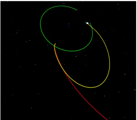
On the last of five Moon flybys, the periapsis altitude of the spacecraft was 120 km. After the flyby, the space probe was into an escape trajectory with a hyperbolic escape velocity of 1.67 km/s (C3 of 2.80 km2_/s2_{) [2]. In 2006, NASA launched two identical spacecraft to study} coronal mass ejections on the Sun. These two probes, STEREO-A and STEREO-B, were launched aboard the same launch vehicle and place in two different heliocentric orbits, one ahead of Earth (STEREO-A) and the other behind (STEREO-B). To achieve these orbits, STEREO-A performs one LGA manoeuvre and STEREO-B two LGA manoeuvres [3]. In figure 1.1 a segment of the STEREO-A and STEREO-B trajectories is displayed. LGA manoeuvres were also used to rescue a communications satellite, AsiaSat 3, in 1998. When a failure occurred in the launch vehicle, the satellite was placed in an unwanted orbit, never reaching the desired geosynchronous orbit. A GEO orbit was then attained through an LGA manoeuvre and the otherwise useless satellite was operation until 2002, although not for the functions originally intended. A study for the ExoMars mission, initially intended to be launched in 2009 or 2011, suggests the use of lunar gravity assist manoeuvres in order to increase mass injected towards Mars. According to this study, a single LGA manoeuvre could increase the mass of the vehicle between 9% and 10.5% and decrease the injection velocity in 120 m/s. In the analysed trajectory where the higher mass was achieved, the manoeuvre would increase the characteristic energy from 8.3 km2_/s2 _{to 10.6 km}2_/s2_{. The} use of multiple lunar gravity assist manoeuvre would increase the mass launched to Mars by 18% to 23% [4].

Figure 1.1: Representations of a segment of the trajectories of STEREO space probes at LGA manoeuvres. Moon’s orbit is represented in green, STEREO-A’s orbit in red and STEREO-B in yellow. At the centre, the

blue dot represents the Earth. (credit: NASA)

Others techniques can be applied to decrease the launch energy along with LGA manoeuvres, in Earth-Mars transfers. If low-thrust systems are used, ballistic escape and ballistic capture orbits may reduce the propellant mass required for Earth-Mars transfer orbits [5]. Lunar Distant Retrograde orbits can also be used to decrease the launch energy [6].

Chapter 1 • Introduction

As it can be seen, LGA can be used to provide cost savings to the several missions. The main objective of this work is to design an Earth-Mars transfer orbit with an LGA manoeuvre for each of the 7 real missions previously described (2001 Mars Odyssey, Mars Exploration Rover-A, Mars Exploration Rover-B, Mars Science Laboratory, Mars Orbiter Mission, Mars Atmosphere and Volatile Evolution, and Trace Gas Orbiter). These trajectories are then compared to the real ones and the variations in the characteristic energy are analysed. Ultimately, it will be studied whether the launch mass could be increased or the launch vehicle changed to a less expensive one, without alter significantly the time of flight of the spacecraft.

The present work is divided as follows:

In Chapter 1, the present chapter, an overview of the exploration of Mars and its motivation was given. A historical review of the use of gravity assist manoeuvres and in particular the lunar ones, was also presented. At the end of the chapter, the objective of the work was explained.

Chapter 2 details the astrodynamics and numerical method used. In the first section of the chapter, the problem of orbital transfer is formulated under the two-body problem. In the second section, the optimisations methods are explained.

Chapter 3 presents the numerical simulations obtained from the methods exposed in Chap-ter 2 and from the software General Mission Analysis Tool (GMAT), and its results are dis-cussed. This is performed first for the direct orbit transfer and then for the trajectory with a lunar gravity assist manoeuvre.

Chapter 4 concludes the dissertation, presenting the established conclusions and recom-mendations for future work.

Chapter 2

Modelling

In this chapter, the astrodynamics models and numerical methods used are explained and is divided into two sections. The first section describes some of the well-known equations in the two-body problem. Since the solutions generated throughout this section will be refined by a computer software, the use of the two-body problem is appropriate, as no perturbations will be relevant enough to cause a large error in the velocity vectors obtained. The second section contains an overview of the optimisations methods utilised.

2.1

Astrodynamics models

In this section, the astrodynamics models used are discussed. First, Kepler’s equation, Lam-bert’s problem and the gravity assist model are described. Next, the patched conic method is presented as a technique through combine all trajectories studied. Later, a special procedure for targeting problems is formulated. At the end of this section, conversion between Keplerian and Cartesian elements is shown and a brief explanation of the epoch format and coordinate system used is presented.

2.1.1

Two-body problem

The motion of a spacecraft with negligible mass under the gravitational influence of an attractive body treated as a point mass, is given by the nonlinear differential equation

d2_r dt2 +

µ

r3r = 0 (2.1)

where µ = Gm and m is the mass of the attractive body. All solutions of equation (2.1) are conic sections as stated by Kepler’s first law.

In the two-body problem the conservation of angular momentum and specific orbital energy is verified. Assuming

dr

dt ≡ ˙r ≡ v,

d2_r

dt2 ≡ ¨r ≡ ˙v, ∥r∥ ≡ r, ∥v∥ ≡ v,

the equation for the specific orbital energy, ξ, is

ξ = 1 2v 2₋µ r =− µ 2a (2.2)

and ξ is sometimes also denoted as energy integral.

The orbit equation presented in equation (2.3) is the polar form of a conic section with the attractive body in one of the focus. The true anomaly, ν, is the angle between r and e. The eccentricity vector is given by equation (2.4).

Chapter 2 • Modelling Astrodynamics models r = p 1 + ecos ν (2.3) e = (v 2_{− µ/r)r − (r · v)v} µ (2.4)

Knowing the specific angular momentum (h = r× v), the semi-parameter (p) is given by

p = h

2

µ = a(1− e

2_{) (2.5)}

Another form for the orbit equation in elliptical orbits can be

r = a(1− e cos E) (2.6)

where r is a function of E, the eccentric anomaly. Equation (2.7) relates the eccentric anomaly and the true anomaly.

tanν 2 = √ 1 + e 1− etan E 2 (2.7)

Although most of the formulae that will be described are refer to the elliptical motion and therefore to the eccentric anomaly, the same relations exist for hyperbolic orbits and for the hyperbolic anomaly (F ) [7] [8]. These relations can be attained from those for the elliptical case by replacing a by−a, E by iF and M by −iM, with i =√−1. The relations between trigono-metric functions and hyperbolic functions presented in equations (2.8) to (2.10) are useful to rearrange the formulas obtained for hyperbolic orbits.

sin(iF ) = i sinh(F ) (2.8)

cos(iF ) = cosh(F ) (2.9)

tan(iF ) = i tanh(F ) (2.10)

2.1.2

Kepler’s equation

The expression (2.11) known as Kepler’s equation, describes the relationship between the time since periapsis and the eccentric anomaly, where n = µ1/2_(1/a)3/2_.

M = E− e sin(E) = n(t − T ) (2.11)

Two practical applications of Kepler’s equation are:

• determination of flight time between two positions in spacecraft’s orbit, and

• determination of spacecraft’s position and velocity at a specific time, once its state in a previous time is known.

Rearranging equation (2.11), the time of flight between two positions, can be expressed as tf light=

(E− E0)− e(sin E − sin E0)

n (2.12)

The propagation of an orbit in the two-body problem, or Kepler’s problem, will now be analysed. Both forward and backwards propagation are possible depending on the desirable final time. In 8

Astrodynamics models Chapter 2 • Modelling

the case of non-perturbed Keplerian motion as the one described in the present chapter, the final state can be determined by analytical solution, not been necessary numerical integration of motion’s equations.

Letting r = [x y z]T _{and v = [ ˙x ˙y ˙z]}T_{, if}

X0= [

r0

v0 ]

is the state vector at t = 0, X(t), for t̸= t0, can be found by solving the transcendental equation (2.11). Two methods will be presented to compute the state vector at t.

The first method uses the relations between true anomaly, eccentric anomaly and mean anomaly (M ). Of the six Keplerian element, the true anomaly is the only variable changing its value. Given ν0, the eccentric anomaly is found through

tanE 2 = √ 1− e 1 + etan ν 2 (2.13)

The initial mean anomaly, M0, is given by Kepler’s equation (2.11) and the mean anomaly at t is

M (t) = M0+ n(t− t0) (2.14)

Then, ν can be obtain by solving Kepler’s equation for E and converting to ν.

The second method uses Lagrange coefficients, also known as f and g functions [9]. The f and gfunctions below described can be used to express the spacecraft’s state given that

[ r v ] = [ f g ˙ f ˙g ] [ r0 v0 ] (2.15)

This functions for E0and E are

f = 1− a r0 (1− cos(∆E)) (2.16) g = t− t0− √ a3 µ(∆E− sin(∆E)) (2.17) ˙ f = − √_µa r0r sin(∆E) (2.18) ˙g = 1−a r(1− cos(∆E)) (2.19) where ∆E = E− E0.

It is necessary to determine the eccentric anomaly from equation (2.11) in the two approaches described. To solve Kepler’s equation for E, Newton’s method can be used [9]. This iterative method is written as

Ek+1= Ek+

M− Ek+ esin Ek

1− e cos Ek

(2.20) and is repeated until the desired precision is achieved. The initial guess can be

E = M + esin M

Chapter 2 • Modelling Astrodynamics models

2.1.3

Lambert’s problem

The problem of finding an orbit that connects two position vectors in a given time, is entitled as Lambert’s problem. Through the solution of this problem, the velocity vectors at the two end-points of the arc become known. The primal use of this problem in the present work is to design transfer orbits. The velocities at the two end-points can be given by equation (2.22) and equation (2.23), which use f and g functions.

v0=

r− fr0

g (2.22)

v = ˙gr− r0

g (2.23)

In this dissertation, an algorithm described in [10] to solve Lambert’s problem was adopted. This method uses universal variables allowing the implementation of the same equations for elliptical orbits and hyperbolic orbits.

2.1.4

Gravity assist model

The spacecraft’s motion around the flyby body, in this case the Moon, is now investigated. In this subsection, coordinates in the selenocentric inertial reference frame are denoted in lower case letters (r and v) and for Earth-centred inertial frame are used upper case ones (R and V ). Thus, r and v in a Moon inertial reference frame are

r(t) = R(t)− R(t)M oon (2.24)

v(t) = V (t)− V (t)M oon (2.25)

In a lunar hyperbolic passage, the incoming hyperbolic excess velocity and the outgoing hyper-bolic excess velocity, in selenocentric coordinates, have the same magnitude (v−_∞ = v+

∞) but

different directions (ˆv−_∞̸= ˆv+_∞). This leads to a variation in the velocity components of the state vector with respect to the Earth. The change in magnitude and direction in an Earth-centred reference frame can be seen in figure 2.1. Assuming that the space vehicle approaches the ce-lestial body from behind (in relation to Moon’s velocity vector), the energy in an Earth-centred reference frame increases. If the approach is in front of the Moon the energy decrease.

VM oon

2β v+∞

v−_∞ V (t1)

V (t2)

Figure 2.1: Diagram of a gravity assist manoeuvre. Increase in spacecraft energy after the flyby.

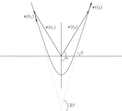
In a flyby, when the motion is examined at a great distance from the Moon (r =∞), the vehicle’s path follows along the hyperbola’s asymptotes, as illustrated in figure 2.2. Considering a ballistic flyby in which the total energy and the angular momentum are unchangeable with respect to the Moon, and knowing that the velocity vector rotates around the angular momentum vector, the velocity after de flyby can be computed from the initial vector. The same occurs for the position vector. This is stated in equation (2.26) and equation (2.27), where the subscripts 1 10

Astrodynamics models Chapter 2 • Modelling 2β β ν v(t1) v(t2) r(t1) r(t2)

Figure 2.2: Diagram of hyperbolic passage.

and2describe components of state vector before and after the flyby, respectively [11].

r(t2) = Roth(2γ)r(t1) (2.26)

v(t2) = Roth(2β)v(t1) (2.27)

The angles γ and β are defined as

γ = π− ν (2.28)

sin β = 1

e (2.29)

In equation (2.31) [9], Euler-Rodrigues formula yields the rotation matrix, introduced in equation (2.26) and equation (2.27), where I is the identity matrix, ˆh≡ u = [u1 u2 u3]T and the matrix

His H =    0 −u3 u2 u3 0 −u1 −u2 u1 0    (2.30)

Roth(ϑ) = I +sin ϑH + (1− cos ϑ)H2 (2.31)

=   

cos ϑ + u2

1(1− cos ϑ) u1u2(1− cos ϑ) − u3sin ϑ u1u3(1− cos ϑ) + u2sin ϑ u1u2(1− cos ϑ) + u3sin ϑ cos ϑ + u22(1− cos ϑ) u2u3(1− cos ϑ) − u1sin ϑ u1u3(1− cos ϑ) − u2sin ϑ u2u3(1− cos ϑ) + u1sin ϑ cos ϑ + u23(1− cos ϑ)

  

Knowing that h· r = 0 and h · v = 0, the rotation matrix can be simplified, resulting in

Roth(ϑ) =   

cos ϑ −u3sin ϑ u2sin ϑ u3sin ϑ cos ϑ −u1sin ϑ −u2sin ϑ u1sin ϑ cos ϑ

 

Chapter 2 • Modelling Astrodynamics models

As a lunar flyby cannot be considered an instantaneous manoeuvre, it is interesting to determine its duration. Since the time of flight from r−_∞to periapsis, and the time of flight from periapsis to r+

∞ are the same, equation (2.12) becomes

tf light= 2

√ −a3

µ (esinh F− F ) (2.33)

Therefore, in Earth-centred reference frame, the spacecraft’s position and velocity post-flyby are R(t2) = R(t2) M oon + Roth(2γ)r(t1) (2.34) V (t2) = V (t2) M oon + Roth(2β)v(t1) (2.35)

2.1.5

Patched conic method

The concept used in the patched conic method is based on the idea that the motion of a space-craft in a multi-body environment can be approached by a conic section around only one planet or moon at each instant [8].

In the case of interplanetary transfer and lunar flyby trajectories, the transfer orbits are divided into several two-body orbits, each one called arc. In an arc the spacecraft is only subject to the gravitational force of the dominant celestial body, no propulsive manoeuvres are applied. The equations for the two body problem are then applied resulting in several Keplerian orbits. This way the mission analysis is simplified. When two arcs are patched together, if no manoeuvre is realised, the continuity of the spacecraft’s state between the two arcs must be ensured (this is attained through the differential correction methods discussed in subsection 2.2.1). A series of arcs with the same dominant body is designated as a leg.

The choice of the body that is considered to be the dominant one, is dictated by its sphere of influence (SOI) and the distance between the space vehicle and that particular celestial body. In equation (2.36) the radius of the sphere of influence of mass m2 relative to mass m1 is shown, with m1 ≫ m2 and where r12 is the distance between the two masses. In table A.1 of the Appendix is presented the radius of the SOI of Earth, Mars and the Moon, as well as some physical data concerning these celestial bodies and the Sun.

rSOI= r12 ( m2 m1 )2/5 (2.36) All arcs obtained in this work are resultant of a Keplerian propagation, a solution of Lambert’s problem or a hyperbolic passage around the Moon.

2.1.6

B-plane targeting

The B-plane targeting technique is primarily used to compute trajectory correction manoeuvres, also known as mid-course manoeuvre, performed by the vehicle in order to correct its trajectory. Small errors in the injection manoeuvre, in the orbit determination or in the dynamical model used, can divert the spacecraft from its desired path. Here, it will be used to produce the initial guess for the lunar gravity assist manoeuvre.

In this coordinate system, shown in figure 2.3, the plane RT is defined so that it is perpendicular 12

Astrodynamics models Chapter 2 • Modelling B-plane _ˆ S ˆ T ˆ R B Orbital Plane Asymptote

Figure 2.3: Geometry of B-plane with spacecraft’s trajectory represented in yellow.

to the approach asymptote and so that it contains the focus of the hyperbola. The B vector is described as the vector from the focus of the hyperbola to the point where the asymptote intersects the B-plane. The S axis has the same direction of the asymptote and the T axis is normal to S and parallel to the ecliptic plane. The R axis completes a right-handed system. The unit vector of the described axes can be written as [12] [13]

ˆ S = cos εe e +sin ε ˆ h× e ∥ˆh × e∥ (2.37) ˆ T = Sˆ× ˆk ∥ ˆS× ˆk∥ (2.38) ˆ R = Sˆ× ˆT (2.39)

where ε = π/2− β and ˆk = [0 0 1]T_{. Then, since}

B = b( ˆS× ˆh) (2.40)

and b =−a√e2− 1, the targeting components (B

T, BR) are expressed as

BT = B· ˆT (2.41)

BR= B· ˆR (2.42)

2.1.7

Keplerian and Cartesian elements

In astrodynamics, it is often necessary to convert the spacecraft state from Cartesian to Keple-rian orbital elements and from KepleKeple-rian to Cartesian ones.

Given the orbital elements, the position and velocity vectors of the spacecraft are [9]

r =

  

r(cos(ω + ν) cos Ω− cos i sin(ω + ν) sin Ω) r(cos(ω + ν) sin Ω− cos i sin(ω + ν) cos Ω)

r(sin(ω + ν) sin i)

 

Chapter 2 • Modelling Numerical methods v =    −µ

h(cos Ω(sin(ω + ν) + e sin ω) + sin Ω(cos(ω + ν) + e cos ω) cos i) −µ

h(sin Ω(sin(ω + ν) + e sin ω)− cos Ω(cos(ω + ν) + e cos ω) cos i) µ

h(cos(ω + ν) + e cos ω) sin i

 

 (2.44)

If the Cartesian state is known then the Keplerian elements can be computed as follows [10]

cos i = hz h (2.45) cos Ω =nx n , if ny< 0, Ω = 2π− Ω (2.46) cos ω =n· e ne , if ez< 0, ω = 2π− ω (2.47) cos ν = e· r er , if r· v < 0, ν = 2π − ν (2.48)

where n = ˆk× h. The semi-major axis and eccentricity are obtained from equation (2.2) and

(2.4), respectively.

Some special cases, such as parabolic orbits, elliptic equatorial orbits and circular inclined and equatorial orbits, are not considered.

2.1.8

Epoch format and coordinate system

The epoch format and the coordinate system adopted were chosen to correspond with those used in GMAT. The selected time format is the Modified Julian Date (MJD) [14].

M J D = (J D− 2430000) + pday (2.49)

The conversion between the Julian Date (JD) and the Gregorian Date format is

J D = 367y− INT ( 7 (y + IN T (m+9₁₂ )) 4 ) + IN T ( 275m 9 ) + d + 1721013.5 (2.50)

where y, m, d, h, min and s are the year, month, day, hour, minutes and seconds respectively, and IN T is truncation of a real number. The term pday (part of the day) in equation (2.49) is

pday= s

60+min

60 + h

24 (2.51)

The coordinate systems used are inertial, with its origin in the respective body and the axes expressed in the MJ2000Eq system, not reported here and described in [14].

2.2

Numerical methods

The following subsections contain an overview of some of the numerical methods used in this dissertation, although in other subsections specific numerical methods can also be described. The present section is divided into two parts: the first presents the differential correction procedure used; in the second, optimisations methods are exposed.

Numerical methods Chapter 2 • Modelling

2.2.1

Differential correction

The two differential correction methods below described, single shooting method and multiple-shooting method, are used to compute the trajectory of the vehicle. These iterative procedures perform small adjust to the spacecraft state in order to achieve a desired final state, Xref. The

initial guess is provided by simplistic models of the two-body problem.

Single shooting method

In this work, the single shooting method is used to compute the velocity vector in a previous state (here called X0), in order to achieve two particular objectives: a position, rref, or some

parameters described in the B-plane coordinate system, BT ref and BRref.

As the initial guess is in the neighbourhood of the solution, Newton’s method is used to derive the single shooting method implemented in the present work. Assuming that the vector w∗ = [w1w2... wn]T is the solution of

f (w∗) = 0 (2.52)

and if w∗is written as

w∗= w + δw (2.53)

then from Taylor series

f (w + δw) = f (w) +∂f (w)

∂w δw +O(δw

2₎

(2.54) Rearranging equation (2.54) and knowing that f (w + δw) = 0, δw can be approximated by

δw ≈ J−1(f (w + δw)− f(w)) (2.55)

δw ≈ −J−1f (w) (2.56)

where J = ∂f (w)/∂w is Jacobian matrix and J−1 its inverse. Therefore

w∗≈ w − J−1f (w) (2.57)

As equation (2.56) is a linearisation of Taylor series in which the high order terms are neglected, an iterative procedure, presented in equation (2.58), can be built to improve the solution.

wk+1= wk− J−1f (wk) (2.58)

In the case where the objective is a specific position, the problem resembles Lambert’s problem, in which it is necessary to determine the initial velocity of an orbit that connects two positions in a given time of flight. However, in Lambert’s problem only the gravitational force of one celestial body is studied (one arc), where with the shooting method the influence of more than one SOI can be considered (multiple arcs). The application of equation (2.58) results in [15]

   ˙ x0 ˙ y0 ˙ z0    k+1 =    ˙ x0 ˙ y0 ˙ z0    k − J−1 k        xf yf zf    k −    x y z    ref     (2.59)

Chapter 2 • Modelling Numerical methods

where the Jacobian matrix is

Jk=      ∂xf ∂ ˙x0 ∂xf ∂ ˙y0 ∂xf ∂ ˙z0 ∂yf ∂ ˙x0 ∂yf ∂ ˙y0 ∂yf ∂ ˙z0 ∂zf ∂ ˙x0 ∂zf ∂ ˙y0 ∂zf ∂ ˙z0      (2.60)

When targeting the B-plane, the procedure becomes    ˙ x0 ˙ y0 ˙ z0    k+1 =    ˙ x0 ˙ y0 ˙ z0    k − J−1 k        BT BR e    k −    BT BR e    ref     (2.61) with Jk=      ∂BT ∂ ˙x0 ∂BT ∂ ˙y0 ∂BT ∂ ˙z0 ∂BR ∂ ˙x0 ∂BR ∂ ˙y0 ∂BR ∂ ˙z0 ∂e ∂ ˙x0 ∂e ∂ ˙y0 ∂e ∂ ˙z0      (2.62)

Finite differences are used to approximate numerically the Jacobian matrix in equation (2.60) and (2.62). Through central difference, the partial derivatives are then

∂f

∂v =

f (v + ∆v)− f(v − ∆v)

2 ∆v (2.63)

In equation (2.63), ∆v is a small value called perturbation, chosen such is small enough so that the partial derivatives in Jacobian matrix are within the linear range but sufficiently large to avoid round-off errors (these errors are present in figure 2.4 for perturbations smaller than 10−13). A test was performed to determine the value of the perturbation to be used. Within the linear range, several values were used to compute the numerical Jacobian matrix for various Earth orbits. These matrices were then compared with the analytic State Transition Matrix (STM) of each orbit. The perturbation value that produced a more accurate Jacobian matrix was selected. This value was 10−7.

10−15 10−14 10−13 10−12 10−11 10−10 10−09 10−08 10−07 10−06 10−05 10−04 10−03 10−02 10−01 −1 −0, 5 0 0, 5 1 1, 5 2 2, 5 3 3, 5 Pertubation Magnitude [km/s] Numerical P artial V alue ∂e/∂ ˙x0 ∂e/∂ ˙y0 ∂e/∂ ˙z0

Figure 2.4: Change in partial derivatives for different perturbations magnitudes.

As seen in equation (2.61) and equation (2.62), a parameter is added to the B-plane targeting scheme, in addition to BT and BR, to generate an invertible Jacobian matrix [13]. The most

Numerical methods Chapter 2 • Modelling

used parameter is the time of closest approach (TCA). However, in this work, the selected parameter was the eccentricity of the orbit with respect to an Earth-centred reference frame. The eccentricity provides a better understanding of transfer orbit than TCA. Another reason is the fact that an orbit with an eccentricity value greater than one ensures that the initial guess and the following approximations produce a trajectory that always reaches the surface of the Earth’s SOI. These are the main reasons for the selection of the eccentricity. The eccentricity, as well as the others two parameters (BT and BR), presents a linear behaviour for 10−13 <

∆v < 10−1in all v components, as observed in figure 2.4.

Multiple shooting method

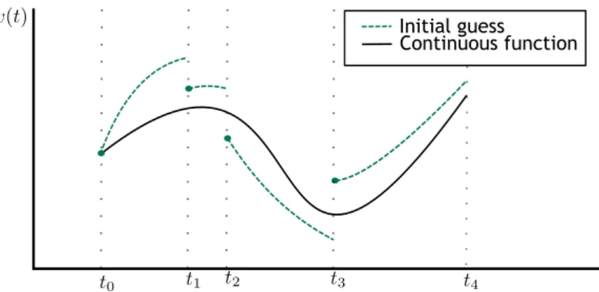
In the multiple shooting method, the trajectory is divided into multiple segments or arcs. Each of these arcs is solved independent taking into account only the point that patch together the segment with the following one. The segments can be as small as required. A representation of multiple shooting methods is presented in figure 2.5.

Initial guess

Continuous function

t0 t1 t2 t3 t4

w(t)

Figure 2.5: Representation of multiple shooting method.

An advantage of multiple shooting method is that, unlike the single shooting method, it does not require a very accurate initial guess for trajectories with lunar gravity assist manoeuvre because is less sensitive to variations caused by hyperbolic passages.

The trajectory of the vehicle must be continuous through time, as no propulsive manoeuvres are applied. Therefore, it is necessary that the position at the end of an arc be the same as the initial position of the arc to follow. In the first approach, single shooting method is used in all arcs. Thus, although the trajectory is continuous, there is a discontinuity in the spacecraft’s velocity at the each patch point[16], which can be removed with nonlinear programming, minimising the angle and amplitude between the two velocity vectors while maintaining the trajectory continuous. Others constraints, such as the periapsis radius in the flyby, can be added. In this dissertation, MATLAB optimisation function fmincon was used to achieve this objective. At the end, the trajectory is refined using single shooting method, to prevent minor discontinuities in the patch points, with initial guess being the one obtained from multiple shooting method. In the present work, it was decided to locate the patch points on the surface of the spheres of influence, respecting the definition of arc presented in section 2.1.5. As an example, if the multiple shooting method is used to compute a trajectory from low Earth orbit to low Moon orbit, this orbit is divided into two segments: the first is from low Earth orbit to the surface of the Moon’s SOI (when the spacecraft is 66170 km away from the Moon); the second segment is from the surface of Moon’s SOI to low Moon orbit.

Chapter 2 • Modelling Numerical methods

This analysis is performed for each of the missions studied.

2.2.2

Optimisation

Two optimisation techniques are used: pruning method and grid search. These two methods are applied together in their most simplistic form and in two level. The first approach or level is used to establish the feasible region of the search space. At the second level the objective is to reduce the region of the solution space [17].

Level I

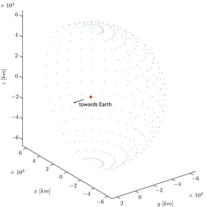
In this level, a grid with 100000 equally spaced points is constructed in the sphere of influence of the Moon in its most distant half from Earth, as illustrated in figure 2.6. These points are, normally, generated for a total of 100 positions of the Moon in its orbit around Earth, corre-sponding to 100 different epochs that are analysed. In this first level, the epochs are usually from 5 days before to 5 days after a hypothetical injection epoch, which would yield the lower lunar periapsis radius possible, and are spaced 1/10 of a day. The difference between the hypo-thetical injection epoch and the actual injection epoch can never exceed 15 days. The velocity vectors of the orbits that connect each of these points to the centre of mass of Mars for each epoch are determined. The trajectory obtained is propagated backwards, performing a lunar flyby, and the perigee radius is then determined.

z [k m ] 6 4 2 0 −2 −4 −6 × 104 × 104 × 104 6 2 4 0 x [km] −2 ₋₄ −6 2 0 −2 −4 −6 y [km] towards Earth

Figure 2.6: Representation of an grid pattern on Moon’s SOI. The Moon is illustrated in orange.

Only points with a perigee radius and a lunar periapsis radius less than 10000 km are of interest. All other points are pruned. The remaining points form a region in space called the feasible region. If there are few or no points in this region, more points can be added to the grid and the interval between epochs can be decreased, otherwise, the first level pruning is concluded. 18

Numerical methods Chapter 2 • Modelling

Level II

The second level begins with the feasible region and epochs obtained in the first level and searches for solutions with lower initial velocity that best suits each mission.

A new grid is generated in the space region found at the previous level and the achieved set of epochs is divided into intervals of 1/100 of a day. As in level I, the velocity vectors, as well as the lunar periapsis radius of each trajectory, are determined. Orbits with a lunar periapsis minor than 500 km and greater than 5000 km are discarded. The search for the optimal solution for each mission will be then restricted to this new space region and new set of epochs. The level II is then concluded.

Analysing these orbits, the epoch at perigee, the eccentricity and BT and BR parameters can

be obtained. These variables will be used for targeting a lunar gravity assist manoeuvre, when searching for the optimal spacecraft’s trajectory that connects a given initial point in low Earth orbit with the Mars’ centre of mass, and performs a lunar flyby to increase its energy, arriving at Mars at the same epoch as the real mission.

Chapter 3

Numerical Simulation

In this chapter, the results and conclusions obtained from numerical simulations are presented. For each mission, the direct transfer orbit is calculated and compared to the real one to validate the approach used. Then, the transfer orbit is computed again but this time with a lunar gravity assist manoeuvre.

3.1

Direct transfer

To prove that the use of the two-body problem for the analysis and design of Earth-Mars direct transfer orbits is appropriate and to validate some of the models and methods described in the previous chapter, the injection velocity for the seven missions will be computed. The velocity vector obtained will be the initial guess provided to the GMAT, where the injection velocity is then determined taking into account the gravitational influence of Sun and all the planets of the solar system (plus the Moon and Pluto), and compared with the real value.

The General Mission Analysis Tool (GMAT) is an open source software developed by NASA’s God-dard Space Flight Center. This software is mainly used to model, analyse and optimise space-craft’s trajectory from low-Earth orbit to deep space missions. It is possible to use the software either by its graphical user interface or by a script language. GMAT has a syntax based on MATLAB. In addition to writing subroutines in its own script language, there are two interfaces to the Python programming language and MATLAB, which allow GMAT to run built-in and user-created functions of both external systems, thereby extending its capabilities. The software was used for orbit determination in some real-life missions such as the Lunar Crater Observation and Sensing Satellite (LCROSS), Acceleration, Reconnection, Turbulence and Electrodynamics of the Moon’s Interaction with the Sun (ARTEMIS) mission, the Lunar Reconnaissance Orbiter (LRO), the Mars Atmosphere Volatile Evolution Mission (MAVEN) and more recently the Origins Spectral Interpretation Resource Identification Security Regolith Explorer (OSIRIS-Rex) mission. It is used by several universities, commercial companies and organisations. Although it is not the mission analysis and optimisation software most used in space mission analysis, it has an active on-line community and an extensive documentation. GMAT is available for Windows, Mac OS and Linux. The first version of GMAT was released in 2007. The R2013b was the first flight qualified version of GMAT [18] [19].

The date and radius of injection, as well as the injection velocity considered real or true, are given by the ephemeris file of each mission in the JPL’s HORIZONS database [1]. These value are presented in table A.3 of the Appendix. The position, velocity and epoch of injection are denoted as r0, v0 and t0 respectively. The ephemeris data of Earth and Mars were obtained from GMAT at intervals of 1/100 of a day and 1/1000 of a day for the Moon.

When design an Earth-Mars direct transfer orbit, the differential correction methods described in the previous chapter are used, particularly the single shooting method. Since the objective is only to find a good approximation in the two-body problem, there is no need to target a specific

Chapter 3 • Numerical Simulation Direct transfer

position in orbit or specific hyperbolic parameters, therefore the position vector of Mars centre of mass is the desired rref. As the method is an iterative procedure, an initial guess for v0

is necessary. This guess is computed in two parts: the magnitude and unit vector. The unit vector of Earth’s velocity gives the direction of the initial guess. The magnitude is computed with a simplified version of the patched conic method. The transfer orbit is divided into the hyperbolic departure phase, the heliocentric phase and the hyperbolic arrival phase. Through Lambert problem, the magnitude of the hyperbolic excess velocity (v_∞) of the departure phase is determined. Then, the magnitude of the injection velocity is computed from the energy integral.

The orbit is propagated using Kepler’s equation to find the position at, tf. Even when the initial

guess is poor, for most cases the single shooting method converges to the solution. When the single shooting method fails, the injection velocity is computed through the multiple shooting method (MSM). For MSM, the trajectory is divided into two arcs. Lambert problem is used to compute the velocity at the beginning of each arc. By varying the location of the patch point on the surface of Earth’s sphere of influence and the time of flight of each arc, an Earth-Mars transfer orbit, continuous both in spacecraft’s position and velocity, is obtained. While iterating

v0, a special attention is given to ensure that the orbit remains hyperbolic with respect to Earth, otherwise, the trajectory does not cross Earth’s sphere of influence and both procedures fail. In GMAT, the injection velocity obtained is used as initial guess to achieve the same hyperbolic parameters as those achieved by the actual spacecraft trajectory. Then, one by one, all celestial bodies previous mentioned are added to the dynamic model to simulate the actual dynamics of an n-body environment, and the trajectory is computed again. Although in GMAT, other forces such as solar radiation pressure or drag, can be added to the dynamic model, none of these forces/perturbations was considered since there is an increase in the computing time and the overall effect on the trajectory caused by such forces is not significant.

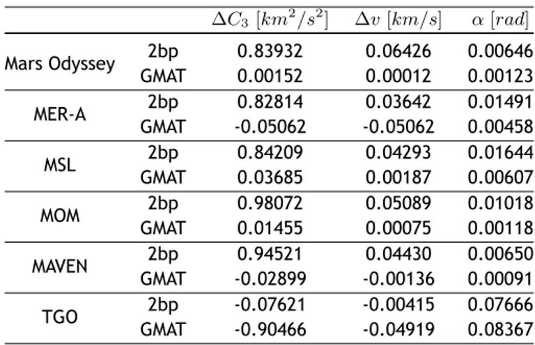
The results obtained from the two methods are exposed in table A.2 of the Appendix. A graphical representation of each of the missions are also present in the Appendix. A comparison between the real values and those determined with the two-body problem (2bp) and with GMAT, is pre-sented in table 3.1. There, the absolute error of the characteristic energy (∆C3), the absolute error of the velocity’s magnitude (∆v) and the angle between the velocity vectors (α), are displayed.

Table 3.1: Absolute error of two-body problem and GMAT results.

∆C3[km2/s2] ∆v [km/s] α [rad] Mars Odyssey 2bp 0.83932 0.06426 0.00646 GMAT 0.00152 0.00012 0.00123 MER-A 2bp 0.82814 0.03642 0.01491 GMAT -0.05062 -0.05062 0.00458 MSL 2bp 0.84209 0.04293 0.01644 GMAT 0.03685 0.00187 0.00607 MOM 2bp 0.98072 0.05089 0.01018 GMAT 0.01455 0.00075 0.00118 MAVEN 2bp 0.94521 0.04430 0.00650 GMAT -0.02899 -0.00136 0.00091 TGO 2bp -0.07621 -0.00415 0.07666 GMAT -0.90466 -0.04919 0.08367

The results of table 3.1 prove that the two-body problem is a good approximation for prelimi-22

Lunar gravity assist trajectory Chapter 3 • Numerical Simulation

nary design of an Earth-Mars transfer orbit. This can be assumed because, unlike the real values that take into account perturbations from several celestial bodies, in the two-body problem only one gravitational force is considered to act on the spacecraft at any given instant, and yet the maximum error in the velocity’s magnitude is 0.06426 km/s, and when comparing the direction of the velocity vectors, five of the six missions reveal an error inferior to 0.01745 rad (approximately 1 degree). As expected, the results obtained from GMAT simulations are nearly identical to the actual values. The small differences can be partially explained by perturbations not taken into account in the GMAT model, but mainly due to the trajectory correction manoeu-vres executed by all spacecraft. The TCM explain the difference as the vehicles had to correct their trajectory to reach the final state recorded in the JPL’s Horizon database. The results of GMAT for the TGO mission present a larger error than for the other missions. This may be due to an error in the time and position considered for the spacecraft injection, not reflecting the actual epoch and position of injection, and not as a result of errors in calculations. From table A.2 can be noted that for TGO results, the difference between the values determined with the 2bp and the values determined with GMAT is the same as for the other missions. This difference to the actual value of the TGO mission does not disprove the results obtained with the GMAT for all other cases analysed.

When comparing the direct transfer orbits with those with a lunar gravity assist manoeuvre, the indicated values of the direct trajectories are those obtained from the GMAT.

3.2

Lunar gravity assist trajectory

The design of an Earth-Mars trajectory with lunar gravity assist manoeuvre is now studied. In this transfer orbit, the spacecraft is injected from the same injection position as before, passes through the Moon and arrives at Mars in the same epoch and with equal hyperbolic parameters, as in the case of direct transfer. The injection epoch may or may not be the same. In the lunar flyby, a special attention is given to ensure that the spacecraft’s periapsis is greater than the equatorial radius of the Moon. In this work, the spacecraft must pass with an altitude superior to 100 km. Another restriction regarding the lunar periapsis is the maximum periapsis radius allowed, which must be inferior to 5000 km. As in the direct transfer, here the final trajectory is also designed with GMAT, using the two-body problem and the multiple shooting method to generate a good initial guess.

The design of the trajectory is divided into two phases. The first phase is the pruning and grid search described in the previous chapter. The second phase is the use of the multiple shooting method for computation of the injection epoch and velocity.

This type of trajectory is discussed in detail for the MER-A mission. For all the others missions, only results and conclusions are presented.

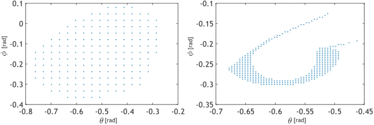
The pruning and grid search begins with a search in the interval between the day 22804 in MJD and day 22815. The results of level 1, shown in figure 3.1, reveal that the feasible region on the Moon’s SOI in spherical coordinates is located at−0.8 rad < θ < −0.2 rad and −0.4 rad <

ϕ < 0.1 rad. The second level explores the region obtained in level 1. With level 2, the feasible

epoch is determined and the feasible region is further reduced. The result of level 2 is also displayed in figure 3.1.

Chapter 3 • Numerical Simulation Lunar gravity assist trajectory

Figure 3.1: Level 1 pruning (left) and level 2 pruning (right).

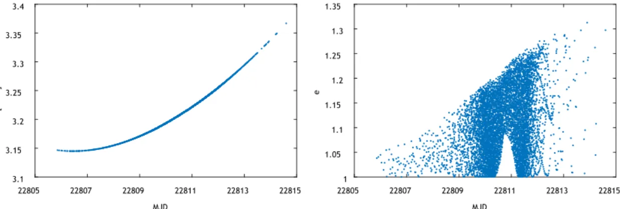
The Moon’s orbit shown in figure 3.2, corresponds to the same interval as the set of epochs determined in level 2. This interval is also shown in figure 3.3, where the velocity’s magnitude for each epoch is displayed. When design the trajectory, the epochs with lower velocities are the first ones targeted by the iterator procedure. After the two levels are completed and the targeting parameters determined, the multiple shooting method is used to compute the trajectory. 10 5 6 x [km] 4 2 0 -5 -3 -1 1 y [km] 3 -2 1 0 -1 5 10 5 10 5 z [km] Lunar periapsis [km] 1000 1500 2000 2500 3000 3500 4000 4500 Earth x x x

Figure 3.2: The feasible region in Earth-centred coordinates. The color bar shows the lunar periapsis radius. The red line represents the Moon’s Orbit.

The transfer orbit is divided into four arcs: the first is from the injection point to the surface of the Moon’s sphere of influence; the second one is the trajectory within Moon’s SOI; the following arc is from the surface of Moon’s SOI to the surface of Earth’s sphere of influence; and the last one, is from Earth’s SOI to Mars’ centre of mass.

The b-plane targeting scheme is used to provide the initial guess to the multiple shooting 24