WORKING PAPER SERIES
Universidade dos Açores Universidade da Madeira
CEEAplA WP No. 05/2012
Comparing the Generalised Hyperbolic and
the Normal Inverse Gaussian Distributions for
the Daily Returns of the PSI20
Sameer Rege
António Gomes de Menezes February 2012
Comparing the Generalised Hyperbolic and the Normal
Inverse Gaussian Distributions for the Daily Returns of
the PSI20
Sameer Rege
CRP Henri Tudor
António Gomes de Menezes
Universidade dos Açores (DEG e CEEAplA)
Working Paper n.º 05/2012
Fevereiro de 2012
CEEAplA Working Paper n.º 05/2012 Fevereiro de 2012
RESUMO/ABSTRACT
Comparing the Generalised Hyperbolic and the Normal Inverse Gaussian Distributions for the Daily Returns of the PSI20
The presence of non-normality, fat-tails, skewness and kurtosis in the distribution of the returns necessitates the fitting of distributions that account for this phenomenon. We fit the Generalized Hyperbolic Distribution and the Normal Inverse Gaussian to the daily returns from the Portuguese Stock Index, the PSI20. We use the EM algorithm for estimating the parameters of the Normal Inverse Gaussian while those of the Generalized Hyperbolic distribution are estimated using the Nelder-Mead algorithm. We find that the Generalized Hyperbolic is a better fit than the Normal Inverse Gaussian as it better estimates the probabilities at the left tail where the losses are concentrated.
Keywords: returns distribution; generalised hyperbolic; normal inverse gaussian; Nelder-Mead; EM algorithm
Sameer Rege CRP Henri Tudor 66 rue de Luxembourg L-4221 Esch-sur-Alzette Luxembourg
António Gomes de Menezes Universidade dos Açores
Departamento de Economia e Gestão Rua da Mãe de Deus, 58
Comparing the Generalised Hyperbolic and the Normal Inverse
Gaussian Distributions for the Daily Returns of the PSI20
Sameer Rege CRP Henri Tudor 66 rue de Luxembourg L-4221 Esch-sur-Alzette Luxembourg [email protected]
António Gomes de Menezes CEEAplA, Universidade dos Açores,
Rua da Mãe de Deus, 58
Ponta Delgada, São Miguel, Açores, Portugal Tel. +351 296 650 084
(Received XX Month Year; final version received XX Month Year)
The presence of non-normality, fat-tails, skewness and kurtosis in the distribution of the returns necessitates the fitting of distributions that account for this phenomenon. We fit the Generalized Hyperbolic Distribution and the Normal Inverse Gaussian to the daily returns from the Portuguese Stock Index, the PSI20. We use the EM algorithm for estimating the parameters of the Normal Inverse Gaussian while those of the Generalized Hyperbolic distribution are estimated using the Nelder-Mead algorithm. We find that the Generalized Hyperbolic is a better fit than the Normal Inverse Gaussian as it better estimates the probabilities at the left tail where the losses are concentrated.
Keywords: returns distribution; generalised hyperbolic; normal inverse gaussian; Nelder-Mead; EM algorithm
Introduction
The presence of non-normality, fat-tails and kurtosis in the distribution of the returns necessitates the fitting of distributions that account for this phenomenon. The Value at Risk (VaR), the maximum permissible loss with a given level of confidence (95% or 99%) over a specified time frame (1 day, 1 week, 1 month) is a function of the probability distribution at the left tail which shows negative returns. Thus a distribution that closely approximates the fat tails is crucial for calculating the VaR. The Generalised Hyperbolic (GH) distribution and its subclass the Normal Inverse Gaussian are two distributions that can possibly account for the fat tails
The generalised hyperbolic distribution being the superset of the normal inverse Gaussian distribution, we expect it ex-ante to be a better fit for the returns data. However it is very expensive in terms of computation.
The paper is structured as follows. The mathematical part gives a succinct description of the two distributions and the various other distributions that are necessary to generate the generalised hyperbolic and normal inverse Gaussian distributions. The characteristic functions of these distributions are linked to their various moments. The maximum likelihood of the distribution function is indispensable in order to obtain expressions for the parameters of the distributions. We use this method to obtain the maximum-likelihood estimates. The estimation part outlines the algorithms used to estimate the parameters. We tabulate the results and discuss the fits of the two distributions to the actual data. The final section concludes. Mathematical Description
The distribution functions, characteristic function and the various moments of the distributions are used to lay the foundation for the estimation of the parameters and
algorithms for simulation. We begin with the generalised hyperbolic and conclude with the normal inverse Gaussian.
Generalised Hyperbolic Distribution
Proposed by Barndorff-Nielsen (1977) the Generalised Hyperbolic [gh(α,β,δ,λ,µ)] distribution is a 5-parameter (change in tails parameterα, , location parameterλ µ , skewness parameterβ , scale parameterδ) Normal Variance-Mean mixture with the Generalised Inverse Gaussian [gig(z|λ,δ,γ)] as a mixing distribution. Formally we have 2 2 z z 2 1 1 ) 1 , 0 | y ( N ~ y e ) ( K 2 z ) , , | z ( gig ~ z ) , , , , | x ( gh ~ x z y z ) x ( gh 2 2 β − α = γ δγ ⎥⎦ ⎤ ⎢⎣ ⎡ δ γ = γ δ λ µ δ λ β α + β + µ = ⎟ ⎟ ⎠ ⎞ ⎜ ⎜ ⎝ ⎛ γ + δ − λ − λ λ
The distribution function is given by
] [ K 2 ) ( ) , , , ( a e ] ) x ( [ K ] ) x ( )[ , , , ( a ) , , , , | x ( gh 2 2 2 / 1 2 / 2 2 ) x ( 2 2 2 / 1 2 / 1 2 2 β − α δ δ α π β − α = µ δ β α µ − + δ α µ − + δ µ δ β α = µ λ δ β α λ λ − λ λ µ − β − λ λ − λ
Where ]Kλ[x is the modified Bessel’s function of the third kind and
0 if | | 0 0 if | | 0 0 if | | 0 < λ α ≤ β > δ = λ α < β > δ > λ α < β ≥ δ
The density of a generalised hyperbolic can be simplified whenλ=1/2, forλ=n+1/2,n =0,1,2,.., the Bessel’s function Kλ(x)is expressed as
⎥ ⎦ ⎤ ⎢ ⎣ ⎡ − + + π =
∑
= − − − + n 1 i i x 2 / 1 2 / 1 n ) x 2 ( !i )! i n ( )! i n ( 1 e x 2 ) x ( Kwe have Kλ(x)=K−λ(x)implying 1/2 1/2 x 1/2e x 2 ) x ( K ) x ( K = − = π − − The characteristic function φx(t)of the distribution is
] [ K ] ) it ( [ K ] it [ e ) t ( 2 2 2 2 2 / 2 2 2 2 t i x β − α δ + β − α δ ⎭ ⎬ ⎫ ⎩ ⎨ ⎧ + β − α β − α = φ λ λ λ µ
The various moments of any distribution are obtained from the characteristic function. Denote ψx(t)=ln[φx(t)] as the natural logarithm of the characteristic function. The various moments are then defined as
[
]
[
'']
2 4 'x''' @t 0 x ''' ' x 0 t @ ''' x 3 2 / 3 '' x ''' x 0 t @ '' x 2 2 2 0 t @ ' x | ) t ( i 1 ) t ( ) t ( kurtosis | ) t ( i 1 ) t ( ) t ( skewness | ) t ( i 1 )] x ( E [ ) x ( E iance var | ) t ( i 1 ) x ( E mean = = = = ψ ψ ψ ψ ψ ψ ψ = − ψ =Where i= −1is the imaginary number and (t), (t), (t), ''''(t)
x ''' x '' x ' x ψ ψ ψ ψ denote the
first, second, third and fourth derivatives respectively of ψx(t)=ln[φx(t)]with respect to t evaluated at t=0. Using the above approach the mean E(x)and the variance
2
σ of the generalised hyperbolic distribution are
⎥ ⎥ ⎦ ⎤ ⎢ ⎢ ⎣ ⎡ β − α δβ β − α δ β − α δ + µ = λ + λ 2 2 2 2 2 2 1 ) ( K ) ( K ) x ( E and 2 2 2 1 2 2 2 2 1 2 2 ,v ) v ( K ) v ( K ) v ( K ) v ( K ) ( ) v ( vK ) v ( K β − α δ = ⎥ ⎥ ⎦ ⎤ ⎢ ⎢ ⎣ ⎡ ⎪⎭ ⎪ ⎬ ⎫ ⎪⎩ ⎪ ⎨ ⎧ ⎥ ⎦ ⎤ ⎢ ⎣ ⎡ − β − α β + δ = σ λ + λ λ + λ λ + λ
Normal Inverse Gaussian (NIG)
2 2 2 2 1 )} x ( { ) x ( ) ) x ( ( K e ) , , | x ( nig 2 2 µ − + δ µ − + δ α π αδ = δµ β α δ α −β +β −µ where x,µ∈R,0≤δ,0≤|β|≤α
The characteristic function of the distribution is given by
µ + + β − α δ − β − α δ = φ ( it) it x 2 2 2 2 e ) t (
The mean E(x)and the variance σ2of the normal inverse gaussian distribution are
2 2 ) x ( E β − α δβ + µ = and 2 2 3/2 2 2 ] [α −β δα + µ = σ
Estimation of distribution parameters
This section briefly describes the estimation procedures used for obtaining the parameters of the normal inverse Gaussian followed by that for the generalised hyperbolic distribution.
Normal Inverse Gaussian (NIG)
For the generalised hyperbolic distribution the mixing distribution is the generalised inverse Gaussian. When
2 1 =
λ , we have the specific case of normal inverse Gaussian
and the mixing distribution is called Inverse Gaussian. The inverse Gaussian
distribution is given by ⎟ ⎟ ⎠ ⎞ ⎜ ⎜ ⎝ ⎛ γ + δ − − δ π δ = γ δ 2 z z 1 2 3 z 2 2 e x e 2 ) , | z (
IG .We use the Expectation-Maximization (EM) algorithm as described by Karlis (2002) for estimating the parameters.
EM Algorithm for estimation of parameters
(1) obtain expression for parameters by maximising log-likelihood
(2) the mixing distribution is inverse Gaussian and need to estimate α,β,δ,µ
(4) we need to calculate z|xand |x z 1
(5) in expectation step [k] obtain z[k] =f
(
α[k],β[k],δ[k],µ[k])
(6) in the maximisation step update
(
α[k],β[k],δ[k],µ[k])
(7) iterate until convergence
Maximization of the log-likelihood to obtain the expressions for the parameters
differentiate the log-likelihood function with respect to the parameters.
⎥ ⎦ ⎤ ⎢ ⎣ ⎡ γ δ β µ = γ µ δ β = µ δ β α
∏
= n 1 i i z i i z | x i i i i,z ) logL( , , , |x ,z ) log f (x |z ; , )f (z | , ) x | , , , ( L logwhere
γ
=α
2 −β
2 . We break the likelihood function into two as follows∏
∏
∏
∏
= ⎥ ⎥ ⎦ ⎤ ⎢ ⎢ ⎣ ⎡ γ + δ − − δγ = = β + µ − − = π δ = γ δ = π = β µ = n 1 i z z 2 1 2 / 3 i n 1 i i z 2 n 1 i i z 2 )] z ( x [ n 1 i i i z | x 1 i 2 2 i 2 i 2 i i e z e 2 ) , | z ( f L 2 z e ) , ; z | x ( f LDifferentiating the log of L with respect to 1
β
,µ
and the log of L with respect to 2δ
γ
, and obtain∑
∑
∑
∑
= = = = − = δ δ = γ − − = β β − = µ n 1 i i _ _ n 1 i i _ n 1 i i _ n 1 i i i _ _ z n z 1 n z z 1 z n z 1 x z x z xE Step Karlis (2002) derives the expressions for the conditional distributions of zi
and i z 1 given i x (1) Define q(x)= δ2 +(x−µ)2
(2) )) x ( q ( K )) x ( q ( K ) x ( q ) x | z ( E i 1 i 0 i i i α α α = (3) )) x ( q ( K )) x ( q ( K ) x ( q ) x | z 1 ( E i 1 i 2 i i i α α α =
M Step having obtained E(zi|xi) and E(z1 |xi)
i obtain the parameters in the following
order for iterations k=1,2,…n
(1)
∑
∑
∑
= = = + − − = β n 1 i i _ n 1 i i _ n 1 i i i ] 1 k [ z 1 z n z 1 x z x (2) µ[k+1] =x_−β[k+1]z_ (3)∑
= + − = δ n 1 i i _ ] 1 k [ z n z 1 n (4) _ ] 1 k [ ] 1 k [ z + + =δ γ (5) α[k+1] =( ) (
γ[k+1] 2 + β[k+1])
2Generalised Hyperbolic Distribution
The likelihood function is
(
)
∑
∑
⎥ ⎥ ⎦ ⎤ ⎢ ⎢ ⎣ ⎡ µ − β + α + ⎥⎦ ⎤ ⎢⎣ ⎡ −λ + λ δ β α = − λ = ) x ( v K log ) v log( 4 1 2 ) , , , ( a log n L i i ) 2 1 ( n 1 i 2 i[ ]
(
δγ)
− δ λ − α ⎥⎦ ⎤ ⎢⎣ ⎡ −λ − π − γ λ = λ δ βα log log log Kλ
2 1 ) 2 log( 2 1 log ) , , , ( a log wherevi = δ2 +(xi −µ)2 and γ= α2 −β2
Differentiating the log likelihood function with respect to the parameters we get Table 1. Maximum likelihood estimates of the generalised hyperbolic distribution
1 = ⇒λ= λ 0 d dL
∑
= λ− − λ λ λ ⎥ ⎥ ⎥ ⎥ ⎦ ⎤ ⎢ ⎢ ⎢ ⎢ ⎣ ⎡ α α + + ⎥ ⎥ ⎦ ⎤ ⎢ ⎢ ⎣ ⎡ δγ δγ − ⎟⎟ ⎠ ⎞ ⎜⎜ ⎝ ⎛ αδ γ n 1 i i 2 1 i ' 2 1 2 i ' 2 ) v ( K ) v ( K ) v log( 2 1 ) ( K ) ( K log 2 1 n 2 = ⇒α= α 0 d dL∑
= λ− − λ λ + λ ⎥ ⎥ ⎥ ⎥ ⎦ ⎤ ⎢ ⎢ ⎢ ⎢ ⎣ ⎡ α α + ⎥ ⎦ ⎤ ⎢ ⎣ ⎡ α ⎟ ⎠ ⎞ ⎜ ⎝ ⎛ −λ − γ αδ δγ δγ n 1 i i i 2 1 i ' 2 1 1 v ) v ( K ) v ( K 1 2 1 ) ( K ) ( K n 3 = ⇒β= β 0 d dL∑
= λ + λ + ⎥ ⎦ ⎤ ⎢ ⎣ ⎡ µ − γ βδ δγ δγ − n 1 i i 1 x ) ( K ) ( K n 4 = ⇒δ= δ 0 d dL∑
= λ− − λ λ + λ ⎥ ⎥ ⎥ ⎥ ⎦ ⎤ ⎢ ⎢ ⎢ ⎢ ⎣ ⎡ δα α α + δ − λ + ⎥ ⎦ ⎤ ⎢ ⎣ ⎡ γ δγ δγ + δ λ − n 1 i i i 2 1 i ' 2 1 2 i 1 v ) v ( K ) v ( K v 2 ) 1 2 ( ) ( K ) ( K 2 n 5 = ⇒µ= µ 0 d dL∑
= λ− − λ ⎥ ⎥ ⎥ ⎥ ⎦ ⎤ ⎢ ⎢ ⎢ ⎢ ⎣ ⎡ α α α + − λ µ − − β − n 1 i i 2 1 i ' 2 1 i i i ) v ( K ) v ( K v 2 ) 1 2 ( v ) x ( nTo obtain the parameter values we use the Nelder-Mead (1965) algorithm. Press, Teukolski, Vetterling and Flannery (1992) outline the procedures for obtaining the values of the Bessel’s function of the third kind which is used to estimate the parameters. To test the goodness of fit we superimpose the simulated data using the estimated parameters.
Results
This section describes the results obtained by fitting the various distributions to data. We start with the data description and the comparison with the normal distribution estimated using the maximum likelihood methods. Later we compare the estimated fits of the generalised hyperbolic and normal inverse Gaussian distributions with respect to the actual values.
Data Description and Normal Distribution
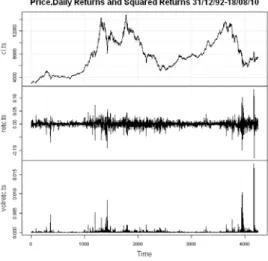
We use the daily closing values of the PSI20 from December 31, 1992 to August 18, 2010 to estimate the distributions. Figure 1 shows the index series (cl.ts), the daily returns series (retc.ts) and the volatility series (square of daily returns: volretc.ts).
Figure 1. Price-Daily Returns and Squared Returns of PSI20
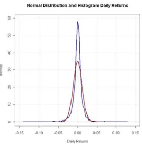
We also fit the normal distribution as a benchmark distribution for comparison with the generalised hyperbolic and normal inverse Gaussian distributions. The maximum likelihood parameters are obtained by equating the sample means and variance to that of the normal. The normal fit superimposed on the density of the actual daily returns is shown in figure 2. The actual returns show a much higher kurtosis and more extreme values as compared to the normal.
Table 1. Parameters Generalised Hyperbolic Distribution
λ α β δ µ
0.1242 78.87 11.98 0.003763 0.000213
Table 2. Parameters Normal Inverse Gaussian Distribution
α β δ µ
54.7202 -3.6800 0.006819 0.000673
Table 1 and Table 2 show the estimated parameters of the Generalisd Hyperbolic and Normal inverse Gaussian distributions respectively. We use these parameters to simulate the distributions to compare with the actual daily returns.
Simulation of normal inverse Gaussian and generalised hyperbolic distributions
Rydberg (1997) suggests a method to obtain data from normal inverse Gaussian
) , , , | x ( f α β δ µ distribution.
(1) Sample zfrom an inverse Gaussian distribution IG(δγ)
(2) Sample yfrom a standard normal Gaussian distribution N(0,1)
(3) Return x =µ+βz+y z
(1) Set γ δ =
τ where γ = α2 −β2 ; λ=δ2and sample 2 1 ~ v χ (2) Compute 1
(
v 4 v ( v)2)
2 z τ − τ λ+ τ λ τ + τ = and 1 2 2 z z = τ (3) Define ) z ( p 1 + τ τ = then ⎩ ⎨ ⎧ − = ) p 1 ( y probabilit with z p y probabilit with z z 2 1We use Scott (2009) in R Development Core Team (2009) for generating the variables from the generalised hyperbolic distribution.
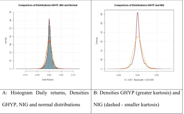
Figure 3. Histogram of Daily Returns and Densities of GHYP, NIG and Normal distribution fit to data
A: Histogram Daily returns, Densities GHYP, NIG and normal distributions
B: Densities GHYP (greater kurtosis) and NIG (dashed - smaller kurtosis)
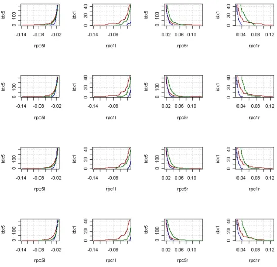
Figure 4 shows the left and right tails for the actual daily returns at 1% and 5% probabilities and compares it with the simulated distribution of the GHYP and the NIG. We ran 10000 simulations of the GHYP and NIG to check whether the left tail for the GHYP performs better than that of the NIG. Our measure of performance was limited to the area under the left tail at 5% and 1% of the actual distribution of the daily returns. We found that the GHYP has a greater area or fatter tails that approximate the actual distribution more closely than the NIG. We find a similar case with the right tail but find that the GHYP has more probability than the actual. Since it is the maximum possible loss that determines the risk we focus on the left tail and find that the GHYP is a better fit than the NIG
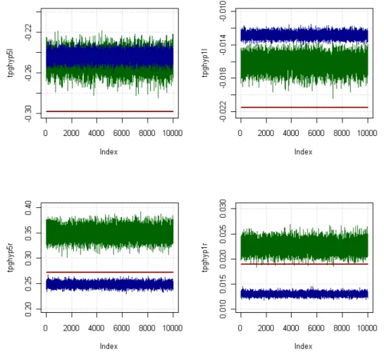
Figure 5 shows the cumulative returns for the actual and the simulated GHYP and NIG distributions for 10000 simulations. The value for each simulation is on the X-axis and the cumulative returns on the Y-X-axis. This is at the 5% and 1% probability of the left and right tails. The flat straight is the value for the actual returns of the daily data and remains flat as it does not change across simulations. The graphs tpghyp5r, tpghyp1r, tpghyp5l and tpghyp1l stand for the cumulative distributions for the GHYP (green) and NIG (blue) at 5% and 1% for the right and left tails respectively. What we observe is that the GHYP is closer to the actual at the 1% at the left tail. At the 5% the GHYP is still closer but there is an overlap with the NIG. For the right tails the GHYP overestimates the probability in the tails as it lies above the actual returns at both 5% and 1%.
Conclusion
We estimated the parameters for the Generalised Hyperbolic and Normal Inverse Gaussian distribution using the Nelder-Mead and Expectation-Maximization algorithms respectively. We find that the generalised hyperbolic distribution is a better fit than the normal inverse Gaussian as it better estimates the probability at the tails, especially the left tails where the losses are concentrated.
Acknowledgements
1. We thank the Direcção Regional da Ciência, Tecnologia e Comunicações for funding the research 2. We thank Prof Gualter Couto for procuring the data on PSI20.
Sameer Rege is a post-doctoral research fellow at the Department of Economics and Business, University of the Azores. He holds a degree in Mechanical Engineering from VJTI, University of Mumbai and a PhD in Economics from IGIDR, Mumbai, India.
António Gomes de Menezes is an Assistant Professor with Aggregation at the Department of Economics and Business, University of the Azores. He has degrees in Economics from the New University of Lisbon, Portugal followed by Masters and PhD degrees in Economics from Boston College, USA
References
Barndorff-Nielsen, O.E., 1977, Exponentially decreasing distributions for the logarithm of particle size. Proceedings of the Royal Society London A 353, 401-419. Karlis, D., 2002. An EM type algorithm for maximum likelihood estimation of the normal-inverse Gaussian distribution, Statistics and Probability Letters
57, 43-52
Nelder, J.A., Mead, R., 1965. A simplex method for function minimization, Computer Journal 7, 308-313
Press, W.H., Teukolsky, S.A., Vetterling, W.T., Flannery, B.P., 1992 Numerical Recipes in C. Cambridge University Press
R Development Core Team, 2009 R: A language and environment for statistical Computing, R Foundation for Statistical Computing, Vienna, Austria ISBN 3-900051-07-0
Rydberg, T.H., 1997. The normal inverse Gaussian Lévy process: Simulation and approximation, Commun. Statist.-Stochastic Models 34, 887-910
Scott, D., 2009, HyperbolicDist: The hyperbolic distribution. Tech. rep., URL