Mitigation of numerical Cerenkov radiation and instability using a hybrid finite difference-FFT Maxwell solver and a local charge conserving current deposit

Contents lists available atScienceDirect

Computer Physics Communications

journal homepage:www.elsevier.com/locate/cpc

Mitigation of numerical Cerenkov radiation and instability using a

hybrid finite difference-FFT Maxwell solver and a local charge

conserving current deposit

Peicheng Yu

a,∗

, Xinlu Xu

b

, Adam Tableman

c

, Viktor K. Decyk

c

, Frank S. Tsung

c

,

Frederico Fiuza

d

, Asher Davidson

c

, Jorge Vieira

e

, Ricardo A. Fonseca

e,f

, Wei Lu

b

,

Luis O. Silva

e

, Warren B. Mori

a,c

a_{Department of Electrical Engineering, University of California Los Angeles, Los Angeles, CA 90095, USA} b_{Department of Engineering Physics, Tsinghua University, Beijing 100084, China}

c_{Department of Physics and Astronomy, University of California Los Angeles, Los Angeles, CA 90095, USA} d_{Lawrence Livermore National Laboratory, Livermore, CA, USA}

e_{GOLP/Instituto de Plasma e Fusão Nuclear, Instituto Superior Técnico, Universidade de Lisboa, Lisbon, Portugal} f_{ISCTE—Instituto Universitário de Lisboa, 1649–026, Lisbon, Portugal}

a r t i c l e i n f o Article history:

Received 11 February 2015 Received in revised form 25 June 2015

Accepted 21 August 2015 Available online 28 August 2015

Keywords:

PIC simulation Hybrid Maxwell solver Relativistic plasma drift Numerical Cerenkov instability Quasi-3D algorithm

a b s t r a c t

A hybrid Maxwell solver for fully relativistic and electromagnetic (EM) particle-in-cell (PIC) codes is described. In this solver, the EM fields are solved in k space by performing an FFT in one direction, while using finite difference operators in the other direction(s). This solver eliminates the numerical Cerenkov radiation for particles moving in the preferred direction. Moreover, the numerical Cerenkov instability (NCI) induced by the relativistically drifting plasma and beam can be eliminated using this hybrid solver by applying strategies that are similar to those recently developed for pure FFT solvers. A current correction is applied for the charge conserving current deposit to ensure that Gauss’s Law is satisfied. A theoretical analysis of the dispersion properties in vacuum and in a drifting plasma for the hybrid solver is presented, and compared with PIC simulations with good agreement obtained. This hybrid solver is applied to both 2D and 3D Cartesian and quasi-3D (in which the fields and current are decomposed into azimuthal harmonics) geometries. Illustrative results for laser wakefield accelerator simulation in a Lorentz boosted frame using the hybrid solver in the 2D Cartesian geometry are presented, and compared against results from 2D UPIC-EMMA simulation which uses a pure spectral Maxwell solver, and from OSIRIS 2D lab frame simulation using the standard Yee solver. Very good agreement is obtained which demonstrates the feasibility of using the hybrid solver for high fidelity simulation of relativistically drifting plasma with no evidence of the numerical Cerenkov instability.

© 2015 Elsevier B.V. All rights reserved.

1. Introduction

Fully relativistic, electromagnetic particle-in-cell (PIC) codes are widely used to study a variety of plasma physics problems. In many cases the solver for Maxwell’s equations in PIC codes use the finite-difference-time-domain (FDTD) approach where the cor-responding differential operators are local. This locality leads to advantages in parallel scalability and ease in implementing bound-ary conditions. However, when using PIC codes to model physics

∗_{Corresponding author.}

E-mail address:tpc02@ucla.edu(P. Yu).

problems, including plasma based acceleration [1] in the Lorentz boosted frame, relativistic collisionless shocks [2,3], and fast igni-tion [4–6] particles or plasmas stream across the grid with speeds approaching the speed of light. In these scenarios, the second or-der FDTD Maxwell solvers support light waves with phase veloc-ities less than the speed of light. This property of the FDTD solver leads to numerical Cerenkov radiation from a single particle that is moving near the speed of light. In addition, when beams or plas-mas are moving near the speed of light across the grid a violent numerical instability known as the numerical Cerenkov instabil-ity (NCI) arises due to the unphysical coupling of electromagnetic modes and the Langmuir modes (main and higher order aliased

beam resonance). The beam resonances are at

ω +

2

πµ/

1t

=

(

k1

+

2

πν

1

/

1x1

)v

0, where

µ

and

ν

1refer to the time and space http://dx.doi.org/10.1016/j.cpc.2015.08.026

aliases,1t and1x1are the time step and grid size, and the plasma

is drifting relativistically at a speed

v

0in the1-direction.

ˆ

The NCI was first studied more than 40 years ago [7]. However, it has received much renewed attention [8–14] since the identifi-cation [15,16] of this numerical instability as the limiting factor for carrying out relativistic collisionless shock simulations [2,3], and Lorentz boosted frame simulations [17–20] of laser wakefield ac-celeration (LWFA) [1].

This early and recent work on the NCI [7–11,16,21] have shown that the NCI inevitably arises in EM-PIC simulations when a plasma (neutral or non-neutral) drifts across a simulation grid with a speed near the speed of light. Analysis shows that it is due to the unphysical coupling of electromagnetic (EM) modes and Langmuir modes (including those due to aliasing). As a result, significant recent effort has been devoted to the investigation and elimination of the NCI so that high fidelity relativistic plasma drift simulations can be routinely performed [10–13,19,20].

In previous work Refs. [9,10], we examined the NCI properties for the second order Yee solver [22], as well as a spectral solver

[23,24] (in which Maxwell’s equation are solved in

multi-dimensional

⃗

k space). We note that what we refer to as simply a

spectral solver, others [25] refer to as a pseuspectral time do-main (PSTD) solver. The NCI theory developed in [9,10] were gen-eral and it could be applied to any Maxwell solver. It was found that in the simulation parameter space of interest the fastest growing NCI modes of these two solvers are the

(µ, ν

1

) = (

0

, ±

1

)

modes,

where

µ

and

ν

1defined above are the temporal aliasing, and

spa-tial aliasing in the drifting direction of the plasma. The

(µ, ν

1

) =

(

0

, ±

1

)

modes for both solvers reside near the edge of the fun-damental Brillouin zone (for square or cubic cells), and can be eliminated by applying a low-pass filter. However, due to the sub-luminal EM dispersion along the direction of the drifting plasma in the Yee solver, the main NCI mode

(µ, ν

1

) = (

0

,

0

)

of the Yee

solver has a growth rate that is of the same order as its

(µ, ν

1

) =

(

0

, ±

1

)

counterpart, and these modes reside close to the modes of physical interest. However, the

(µ, ν

1

) = (

0

,

0

)

NCI mode in the

spectral solver has a growth rate one order of magnitude smaller than the

(µ, ν

1

) = (

0

, ±

1

)

modes due to the superluminal

disper-sion of spectral (FFT based) solver. Furthermore, as shown in [10] these

(µ, ν

1

) = (

0

,

0

)

modes can be moved farther away from the

physics modes and their harmonics by reducing the time step in the spectral solver, and can be fully eliminated by slightly modify-ing the EM dispersion in the spectral solver. Usmodify-ing these methods, it was demonstrated in [10] that a spectral EM-PIC can perform high fidelity simulations of relativistically drifting plasmas where the LWFA physics is highly nonlinear with no evidence of the NCI. A multi-dimensional spectral Maxwell solver has a superlumi-nal dispersion relation in all the propagation directions. This is due to the fact that the first order spatial derivatives in the Maxwell’s equation are greater than Nth order accurate (where N is the num-ber of grids) since we are solving the Maxwell’s equation in

⃗

k

space. This superluminal dispersion relation leads to highly local-ized

(µ, ν

1

) = (

0

,

0

)

NCI modes and the reduction of their growth

rates (compared with their Yee solver counterpart). In this paper, we propose to use a hybrid Yee-FFT solver, in which the FFT is per-formed in only one direction, namely the drifting direction of the plasma, while keeping the finite difference form of the Yee solver in the directions transverse to the drifting direction. In other words, EM waves moving in the1 direction will have a superluminal dis-

ˆ

persion (due to the Nth order accurate spatial derivatives) while those moving in the2 (and

ˆ

3 in 3D) directions will have a sublu-

ˆ

minal dispersion due to the second-order-accurate spatial deriva-tives. The advantages of this approach over a fully spectral solver is that the field solver is local in the transverse directions so that bet-ter parallel scalability than a fully FFT based solver can be achieved

(assuming the same parallel FFT routines are used). In addition, it is easier to include a single FFT into the structure of mature codes such as OSIRIS [26]. Furthermore, this idea works well with a quasi-3D algorithm that is PIC in r

−

z and gridless in

φ

[27,28], where the FFTs cannot be applied in ther direction. We note that re-

ˆ

cently a method for achieving improved scalability for FFT based solvers was proposed [25] in which FFTs are used within each local domain, but it introduces as yet unquantified errors in the longi-tudinal fields. The relative advantages and tradeoffs between the variety of approaches being proposed will be better understood as they begin to be used on real physics problems.

We use the theoretical framework for the NCI developed in Refs. [9,10] to study the NCI of the hybrid solver. As we show be-low, the fastest growing NCI modes for the proposed hybrid solver behave similarly to those for the spectral solver. In

⃗

k space they

reside at the edge of the fundamental Brillouin zone for square or cubic cells. More importantly, the

(µ, ν

1

) = (

0

,

0

)

NCI mode for

the hybrid solver has almost the same properties (pattern, growth rates) as that of a spectral solver. The NCI can therefore be effi-ciently eliminated in the hybrid solver by applying the same strat-egy as in the spectral solver. Moreover, simulations have shown that the NCI properties of the quasi-3D r

−

z PIC and gridless in

φ

algorithm [27,28] are similar to that of 2D Cartesian geometry [29]. Therefore, the idea of a hybrid Yee-FFT solver can be readily applied to quasi-3D geometry. We also note that the use of local FFTs in do-mains along z [25] could also be used within the hybrid approach described here.

In this paper, we first discuss the algorithm for the hybrid Yee-FFT Maxwell solver in Section2. In Section3, we apply the the-oretical framework in Refs. [9,10] to study the NCI properties of the hybrid solver analytically and in PIC simulations. We compare OSIRIS [26] results with the hybrid solver against UPIC-EMMA [11] results with a fully spectral (FFT based) solver. In Section4, it is shown that the strategies used to eliminate the NCI for purely spec-tral solvers are also valid for the hybrid solver. In Section5, we extend the hybrid solver idea to the quasi-3D algorithm in OSIRIS and present simulation studies of the NCI properties in this geom-etry. We then present 2D OSIRIS simulations of LWFA in a Lorentz boosted frame using the new hybrid solver. Very good agreement is found when comparing simulation results using the hybrid solver in OSIRIS against results from 2D lab frame OSIRIS using Yee solver

and 2D Lorentz boosted frame UPIC-EMMA [11] simulations

us-ing spectral solver. Last, in Section7we summarize the results and mention directions for future work.

2. Hybrid Yee-FFT solver

The basic idea of the hybrid Yee-FFT solver is that the theoret-ical framework developed in [9,10] indicates that the NCI is easier to eliminate when EM waves are superluminal along the direction of the plasma drift. This can be accomplished with higher order solvers or with an FFT based solver in the drifting direction of the plasma (denoted as1-direction). We note that it is more difficult to

ˆ

satisfy strict charge conservation (Gauss’s law) for higher order fi-nite difference solvers by modifying the charge conserving current deposition in real space. Here we replace the finite difference oper-ator of the first spatial derivative

∂/∂

x1in the Maxwell’s equation

in Yee solver with its FFT counterpart that has an accuracy greater than order N. We then correct for this change in the current de-posit to maintain strict charge conservation. Without loss of gen-erality, in the following we will briefly describe the algorithm of the Yee-FFT solver in two-dimensional (2D) Cartesian coordinate. The straightforward extension to the 3D Cartesian case is also dis-cussed.

2.1. Algorithm

We start from the standard algorithm for a 2D Yee solver, in which the electromagnetic fields

⃗

E and

⃗

B are advanced by solving

Faraday’s Law and Ampere’s Law:

Bn+ 1 2 1,i1,i2+1₂

=

B n−1₂ 1,i1,i2+1₂

−

c1t

×

E₃n_,i1,i2+1

−

E₃n_,i1,i2 1x2 (1) Bn+ 1 2 2,i1+1₂,i2

=

B n−1₂ 2,i1+1₂,i2

+

c1t

×

E₃n_,i1+1,i2

−

E₃n_,i1,i2 1x1 (2) Bn+ 1 2 3,i1+1_2,i2+1₂

=

B n−1₂ 3,i1+1_2,i2+1₂

−

c1t

×

En 2,i1+1,i2+1₂

−

E n 2,i1,i2+1₂ 1x1

+

c1t

×

En 1,i1+1_2,i2+1

−

E n 1,i1+1_2,i2 1x2 (3) En+1 1,i1+1₂,i2

=

E n 1,i1+1₂,i2

−

4

π

1t

×

j n+1₂ 1,i1+1₂,i2

+

c1t

×

Bn+ 1 2 3,i1+1₂,i2+1₂

−

B n+1₂ 3,i1+1₂,i2−1₂ 1x2 (4) En+1 2,i1,i2+1₂

=

E n 2,i1,i2+1₂

−

4

π

1t

×

j n+1₂ 2,i1,i2+1₂

−

c1t

×

Bn+ 1 2 3,i1+1₂,i2+1₂

−

B n+1₂ 3,i1−1₂,i2+1₂ 1x1 (5) E₃n_,+_i11_,i2

=

E₃n_,i1,i2

−

4

π

1t

×

jn+ 1 2 3,i1,i2

+

c1t

×

Bn+ 1 2 2,i1+1₂,i2

−

B n+1₂ 2,i1−1₂,i2 1x1

−

c1t

×

Bn+ 1 2 1,i1,i2+1₂

−

B n+1₂ 1,i1,i2−1₂ 1x2 (6) where the EM fieldE and

⃗

⃗

B, and current

⃗

j are defined with the

proper half-grid offsets according to the Yee mesh [22]. If we per-form a Fourier transper-form of Eqs.(1)–(6)in both x1and x2, and in

time, Maxwell’s equations reduce to

[

ω]⃗

B

= −[⃗

k

] × ⃗

E (7)

[

ω]⃗

E

= [⃗

k

] × ⃗

B

+

4

π⃗

j (8) where

[⃗

k

] =



sin

(

k11x1

/

2

)

1x1

/

2

,

sin

(

k21x2

/

2

)

1x2

/

2

,

0



[

ω] =

sin

(ω

1t

/

2

)

1t

/

2

.

(9)

In vacuum where

⃗

j

=

0, the corresponding numerical dispersion relation for the EM waves is

[

ω]

2

=

c2

([

k

]

2₁

+ [

k

]

2₂

).

(10)

The idea of a hybrid Yee-FFT solver is to keep the finite differ-ence operator

[

k

]

₂

=

sin

(

k21x2

/

2

)/(

1x2

/

2

)

in the directions

transverse to the drifting direction, while replacing the finite dif-ference operator

[

k

]

₁ in the drifting direction with its spectral counterpart

[

k

]

₁

=

k1. To achieve this, in the hybrid solver we will

solve Maxwell’s equations in k1space. The current is deposited

lo-cally using a rigorous charge conserving scheme that is equivalent to [30]. For the EM field and current, we first perform an FFT along

x1so that all fields are defined in

(

k1

,

x2

)

space. After that we apply

a correction to the current in the drifting direction

˜

_jn+12 1

=

sin k11x1

/

2 k11x1

/

2 jn+ 1 2 1 (11)

where

˜

j1is the corrected current. In [25], the current is also

cor-rected where they combine a pure FFT solver with a charge con-serving current deposit. This correction ensures that Gauss’s Law is satisfied throughout the duration of the simulation if it is satis-fied initially, as will be discussed in more detail in Section2.3. After the current correction we advance the EM field as

Bn+ 1 2 1,κ1,i2+1₂

=

B n−1₂ 1,κ1,i2+1₂

−

c1t

×

E₃n_,κ1,i2+1

−

En_3,κ1,i2 1x2 (12) Bn+ 1 2 2,κ1,i2

=

B n−1₂ 2,κ1,i2

−

i

ξ

+ k1c1tE3n,κ1,i2 (13) Bn+ 1 2 3,κ1,i2+1₂

=

B n−1₂ 3,κ1,i2+1₂

+

i

ξ

+ k1c1tE₂n_,κ1,i2+1 2

+

c1t

×

E n 1,κ1,i2+1

−

E1n,κ1,i2 1x2 (14) E₁n_,κ+1_1,i2

=

E₁n_,κ1,i2

−

4

π

1t

× ˜

jn+ 1 2 1,κ1,i2

+

c1t

×

Bn+ 1 2 3,κ1,i2+1₂

−

B n 3,κ1,i2−1₂ 1x2 (15) En+1 2,κ1,i2+1₂

=

E n 2,κ1,i2+1₂

−

4

π

1t

×

j n+1₂ 2,κ1,i2+1₂

+

i

ξ

−k1c1tB n+1₂ 3,κ1,i2+1₂ (16) E₃n_,κ+1_1,i2

=

E₃n_,κ1,i2

−

4

π

1t

×

jn+ 1 2 3,κ1,i2

−

i

ξ

− k1c1tB n+1₂ 2,κ1,i2

−

c1t

×

Bn 1,κ1,i2+1₂

−

B n 1,κ1,i2−1₂ 1x2 (17) where k1

=

2

πκ

1

/

N and N is the number of grids in x1direction,

and

κ

1

=

0

,

1

, . . . ,

N

/

2

−

1 is the mode number. Note in the hybrid

solver, the EM fields

⃗

E,

⃗

B, and current

⃗

j have the same temporal and

spatial centering as in the Yee solver, and

ξ

±

₌

exp



±

k11x1 2 i



(18) is the phase shifting due to the half grid offsets of the E1, B2,3, and

j1in the1-direction. Compared with the standard Yee solver algo-

ˆ

rithm, it is evident that if we replace

−

ik1with the corresponding

finite difference form we can recover the standard 2D Yee algo-rithm. We note for this method one can use a different

[

k

]

₁, e.g. the

[

k

]

₁proposed in [31], to allow error-free vacuum EM dispersion in

ˆ

1-direction.

2.2. Courant condition

The Courant condition of the hybrid solver can be easily derived from the corresponding numerical EM dispersion Eq.(10). Substituting into Eq.(10)the finite difference operator in time

[

ω]

[

ω] =

sin

(ω

1t

/

2

)

1t

/

2 (19)

and the finite difference operators in space

[

k

]

₁

=

k1

[

k

]

2

=

sin

(

k21x2

/

2

)

1x2

/

2

(20) we can obtain the corresponding constraint on the time step 1t 2



k2 1

+



sin

(

k21x2

/

2

)

1x2

/

2



2

≤

1

.

(21)

Note the

⃗

k range of the fundamental Brillouin zone is

|

k1

|

≤

π/

1x1,

|

k2

| ≤

π/

1x2, we can obtain the Courant limit on the

hybrid solver 1t

≤

2



π2 1x2₁

+

4 1x2₂

.

(22)

For square cells with1x1

=

1x2, this reduces to1t

≤

0

.

5371x1.

2.3. Charge conservation

In the hybrid Yee-FFT solver, we rely on the Faraday’s Law and Ampere’s Law to advance the EM field. On the other hand, the local charge conserving current deposition [30] ensures the second-order-accurate finite difference representation of the continuity equation,

∂

∂

t

ρ

n i1,i2

+

jn+ 1 2 1,i1+1₂,i2

−

j n+1₂ 1,i1−1₂,i2 1x1

+

jn+ 1 2 2,i1,i2+1₂

−

j n+1₂ 2,i1,i2−1₂ 1x2

=

0 (23) is satisfied, where

∂

∂

tG n

₌

Gn +1

₋

_Gn 1t (24)

where Gn _{is an arbitrary scalar quantity. Therefore, when}

combining this scheme with the second order accurate Yee solver, Gauss’s Law is rigorously satisfied at every time step if it is satisfied at t

=

0. However, when the hybrid solver is used together with the charge conserving current deposition scheme, we need to apply a correction to the current, as shown in Eq.(11), in order that the Gauss’s Law is satisfied at every time step. This can be seen by first performing Fourier transform in the x1direction for Eq.(23),

∂

∂

t

ρ

n κ1,i2

−

i sin

(

k11x1

/

2

)

1x1

/

2 jn+ 1 2 κ1,i2

+

jn+ 1 2 2,κ1,i2+1₂

−

j n+1₂ 2,κ1,i2−1₂ 1x2

=

0 (25) then applying the divergence operator of the hybrid solver to the left and right hand side of the Ampere’s Law, Eqs.(15)–(17). Using Eq.(25), we obtain

∂

∂

t



−

4

πρ

_κn_1,i2

−

ik1E1n,κ1,i2

+

En 2,κ1,i2+1₂

−

E n 2,κ1,i2−1₂ 1x2



=

0 (26) which shows that if Gauss’s Law for the 2D hybrid solver given by

−

ik1E1n,κ1,i2

+

En 2,κ1,i2+1₂

−

E n 2,κ1,i2−1₂ 1x2

=

4

πρ

_κn_1,i2 (27) is satisfied at t

=

0, it is satisfied at each time step.

2.4. 3D Cartesian geometry

It is straightforward to extend the hybrid solver to 3D Carte-sian geometry. In 3D CarteCarte-sian coordinates, we solve Maxwell’s equation in

(

k1

,

x2

,

x3

)

space where we use the same second order

accurate finite difference form of the Yee solver in the2 and

ˆ

3 direc-

ˆ

tions. As in the 2D Cartesian case, the current correction is applied to j1to ensure the Gauss’s Law is satisfied. We have implemented

the hybrid solver in 2D and 3D with current correction in our finite-difference-time-domain (FDTD) code OSIRIS [26].

3. Numerical Cerenkov instability

To investigate the NCI properties of the hybrid solver, we first consider its corresponding numerical dispersion relation. Employing the general theoretical framework established in

Table 1

Crucial simulation parameters for the 2D relativistic plasma drift simulation. npis the reference plasma density, andω2

p=4πq 2_n p/me, kp=ωp(c is normalized to 1). Parameters Values grid size(kp1x1,kp1x2) (0.2,0.2) time stepωp1t 0.41x1

boundary condition Periodic

simulation box size(kpL1,kpL2) 51.2×51.2 plasma drifting Lorentz factor γ =50.0

plasma density n/np=100.0

Refs. [9,10], we can calculate in detail the NCI modes for any Maxwell solver. The roots of the numerical dispersion relation that lead to the NCI can be found numerically by solving Eq. (17) in [9], or by the analytical expression in Eq. (19) of [10]. For convenience we present the corresponding numerical dispersion and analytical expressions of Eq. (17) of [9] inAppendix. For the Yee solver the k space representation of the finite difference operator is

[

k

]

_i

=

sin

(

ki1xi

/

2

)

1xi

/

2

(28) where i

=

1

,

2 in 2D. Meanwhile, in the hybrid solver the

⃗

k

space operator in the drifting direction is replaced with that of the spectral solver

[

k

]

₁

→

k1. By substituting the respective operators

for each direction into Eq. (19) of Ref. [10] [or Eq.(A.4)inAppendix], we can rapidly find the set of NCI modes for the hybrid solver. In

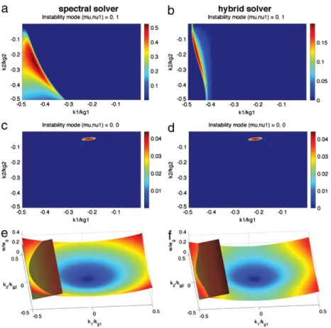
Fig. 1(a)–(d), we plot the

(µ, ν

1

) = (

0

,

0

)

and

(µ, ν

1

) = (

0

, ±

1

)

modes for the hybrid and spectral solvers by scanning over the

(

k1

,

k2

)

space in the fundamental Brillouin zone and solve for the

growth rates of the corresponding unstable modes. The parameters used to generate this plot are listed inTable 1.

We can see fromFig. 1(a) and (b) that the

(µ, ν

1

) = (

0

, ±

1

)

NCI

modes of the two solvers reside near the edge of the fundamental Brillouin zone, although the patterns are slightly different due to their different finite difference operators in the2-direction, which

ˆ

leads to the slightly different EM dispersion curves. InFig. 1(e) and (f) we show how different EM dispersion curves leads to different

(µ, ν

1

) = (

0

, ±

1

)

NCI modes for the two solvers. These modes are

distinct, and far removed from the modes of physical interest, and are relatively easy to eliminate.

More importantly, we see fromFig. 1(c) and (d) that the hybrid solver leads to

(µ, ν

1

) = (

0

,

0

)

NCI modes that are very similar

to their spectral solver counterpart. The pattern of the

(µ, ν

1

) =

(

0

,

0

)

modes for these two solvers are both four dots (in 2D) and highly localized in the fundamental Brillouin zone. We also use the theory to perform parameter scan to study the dependence of growth rates (of the fastest growing mode) and the locations in

k space of the

(µ, ν

1

) = (

0

,

0

)

modes on1t

/

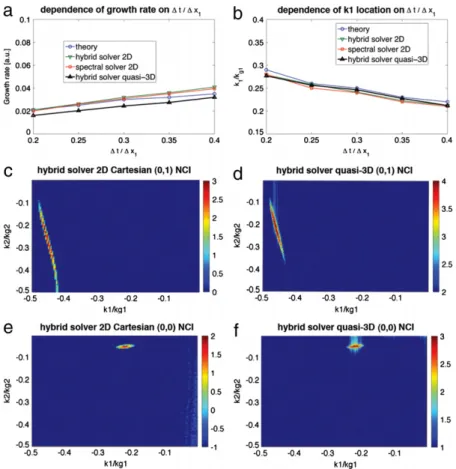
1x1for the hybrid

solver, and compare this result against that of the fully spectral solver, as shown inFig. 2(a) and (b). We likewise carried out OSIRIS simulations using the hybrid solver and UPIC-EMMA [11,32] using the spectral solver, to compare against theoretical results. Very good agreement is found between theory and simulations.Fig. 2(a) and (b) shows that both the k1location, and growth rates of the

(µ, ν

1

) = (

0

,

0

)

modes are almost identical for the two solvers.

This indicates that, just like the spectral solver, the growth rate of the

(µ, ν

1

) = (

0

,

0

)

modes of the hybrid solver is reduced, while

their location in k1increases when the time step is reduced.

In Fig. 2(c) and (e) we show the locations of the unstable

(µ, ν

1

) = (

0

, ±

1

)

, and

(µ, ν

1

) = (

0

,

0

)

NCI modes for the

hybrid solver in OSIRIS for 2D Cartesian geometry. The agreement betweenFigs. 2(c) and1(b), and betweenFigs. 2(e) and1(d) are excellent.

The main advantage of the purely spectral solver regarding its NCI properties in comparison to a purely FDTD solver is that the

Fig. 1. The pattern of the(µ, ν1) = (0, ±1)modes for the two solvers are shown in (a) and (b). The pattern of the(µ, ν1) = (0,0)modes for two solvers are shown in (c) and (d). The intersection between the EM dispersion relations with the first spatial aliasing beam modes for the full spectral solver and the hybrid solver are shown in (e) and (f). When generating these plots we use1x1=1x2=0.2k

−1

0 , and1t=0.08ω −1

0 . Other parameters are listed inTable 1.

superluminal dispersion relation makes it much easier to eliminate the NCI modes at

(µ, ν

1

) = (

0

,

0

)

: the modes have a growth rate

that is one order of magnitude smaller than that for the

(µ, ν

1

) =

(

0

, ±

1

)

modes, their locations are highly localized in

⃗

k space, and

they can be moved away from the modes of physical interest by reducing the time step. We showed above that similar NCI properties can be achieved by using a hybrid FDTD-spectral solver, where the Maxwell’s equation are solved in Fourier space only in the direction of the plasma drift. Comparing with an EM-PIC code using a multi-dimensional spectral solver which solves Maxwell’s equation in

⃗

k space, there are advantages when solving it in

(

k1

,

x2

)

space in 2D [and

(

k1

,

x2

,

x3

)

space in 3D]. Firstly, the hybrid solver

saves the FFT in the other directions; secondly, since the solver is FDTD in the directions transverse to the drifting direction, it is easier to integrate the algorithm into existing FDTD codes such as OSIRIS where the parallelizations and boundary conditions in the transverse direction can remain untouched. Last but perhaps most important, the idea that one can obtain preferable NCI properties by solving Maxwell’s equation in k1space in the drifting direction

can be readily extended to the quasi-3D algorithm [27], as we can solve the Maxwell’s equation in

(

k1

, ρ, ψ)

space.

4. Elimination of the NCI modes

In Ref. [10], we proposed strategies to eliminate the NCI in the spectral solver. These strategies can be readily applied to the hybrid solver. For square (or cubic) cell, the pattern of the fastest growing modes resides in a narrow range of k1near the edge of

the fundamental Brillouin zone. Therefore we can apply a low-pass filter in k1to the current to eliminate the fastest growing modes.

Since the fields are already in k1space when solving the Maxwell’s

equations, the filtering can be done efficiently by applying a form factor to the current only in k1.

As for the

(µ, ν

1

) = (

0

,

0

)

mode, if they are near the main or

higher order harmonics of the physical modes, we can move them away and reduce their growth rates by simply reducing the time step. To further mitigate the

(µ, ν

1

) = (

0

,

0

)

NCI modes when they

are far away from the physical modes, one can modify the EM dis-persion relation, according to the procedure described in Ref. [10], to completely eliminate them. InFig. 3we plot how the modifi-cation is accomplished in the hybrid solver. As shown inFig. 3(a) except for the bump region for most k1the

[

k

]

1for a particular k1is

k1itself; near the bump, the

[

k

]

1for k1is k1

+

1kmod, where1kmod

is a function of k1with

1kmod

=

1kmod,maxcos



k1

−

k1m k1l

−

k1m

π

2



2 (29) where k1l, k1uare the lower and upper k1to be modified, k1m

=

(

k1l

+

k1u

)/

2, and1kmod,maxis the maximum value of1kmod. The

values of k1l, k1uand1kmod,maxare determined by the position of

the

(µ, ν

1

) = (

0

,

0

)

modes and their growth rates. According to

the NCI theory, for the parameters inTable 1, when the

[

k

]

₁is as defined inFig. 3(a) (with k1l

/

kg1

=

0

.

15, k1u

/

kg1

=

0

.

26, and

1k_mod,max

/

k_g1

=

0

.

01), there is no unstable

(µ, ν

₁

) = (

0

,

0

)

NCI modes, i.e., the

(µ, ν

1

) = (

0

,

0

)

mode has a theoretical growth

rate of zero. To verify the theoretical results in the hybrid solver, in

Fig. 3(b) we plot the E₂energy growth with and without the mod-ification. In these simulations we used the parameters inTable 1. The blue curve inFig. 3(b) represents the case without the modifi-cation, while the red and black curves are those with the modifica-tion to k1. The cases with blue and red curves used quadratic

par-ticle shapes, while the case for the black curve used cubic parpar-ticle shapes. We have likewise plotted the E2spectra at the time point

Fig. 2. In (a) and (b) the dependence of the growth rate and k1for the fastest growing(µ, ν1) = (0,0)mode on the time step is shown. The four lines correspond to the theoretical prediction for the hybrid solver in 2D, results from OSIRIS and UPIC-EMMA simulations for the spectral and hybrid solvers in 2D Cartesian geometry, and results for the hybrid solver in the quasi-3D geometry (where the k2is obtained from a Hankel transform). In (c)–(f) the spectrum of E2(Eρ) is plotted for OSIRIS simulations with the hybrid solver in 2D Cartesian or the quasi-3D geometry. In (c) and (d) results from runs where no filter in k1is used to eliminate the(µ, ν1) = (0, ±1)modes. In (e) and (f) a filter in k1was used to eliminate the(µ, ν1) = (0, ±1)modes and now the(µ, ν1) = (0,0)modes are seen. These results show that the 2D Cartesian and quasi-3D geometries have very similar properties and that the strategies used to eliminate the NCI in 2D Cartesian can be applied to the quasi-3D case.

t

=

3200

ω

−₀1indicated inFig. 3(c) and (d) for the two cases with the modifications (red and black curves in3(b)). We can see from

Fig. 3(b) and (c) that after the modification, the growth rate of the

(µ, ν

1

) = (

0

,

0

)

NCI modes reduces to zero. Meanwhile, the red

curve rises later in time due to the

(µ, ν

1

) = (±

1

, ±

2

)

NCI modes.

As we showed in Ref. [10] the growth rate of these higher order modes can be reduced by using higher order particle shape. There-fore when cubic particle shapes are used, as is the case for the black curve, the

(µ, ν

1

) = (±

1

, ±

2

)

NCI modes do not grow

exponen-tially and are therefore much less observable in the corresponding spectrum at t

=

3200

ω

−₀1inFig. 3(d) as compared to3(c). 5. hybrid solver in quasi-3D algorithm

As mentioned in Section1, the idea of the hybrid solver can be easily incorporated into the quasi-3D algorithm [27,28] in which the fields and current are expanded into azimuthal Fourier modes. We can obtain the hybrid Yee-FFT solver for the quasi-3D algorithm by using FFTs in the z (x1) direction and finite difference operators

in r (x2) direction in the equations for each azimuthal mode. Note

in quasi-3D OSIRIS we use a charge conserving current deposition scheme for the Yee solver (as described in [28]), therefore for the hybrid solver adapted for the quasi-3D algorithm we can apply the same current correction for the use of FFTs to j1in order that the

Gauss’s Law is satisfied throughout the duration of the simulation. The NCI properties of the hybrid solver for the quasi-3D algo-rithm are similar to that of the 2D Cartesian geometry [29]. While a rigorous NCI theory for the quasi-3D algorithm is still under de-velopment, we can empirically investigate the NCI for this geome-try through simulation. InFig. 2(d) and (f) we plot the Erdata at a

time during the exponential growth of the EM fields due to the NCI, which shows the

(µ, ν

1

) = (

0

, ±

1

)

and

(µ, ν

1

) = (

0

,

0

)

modes for

the hybrid solver in quasi-3D geometry. For the Erdata, we conduct

an FFT in x1and a Hankel transform in x2. Similarly to the 2D

Carte-sian case, we isolate the

(µ, ν

1

) = (

0

,

0

)

modes by applying a

low-pass filter in the current in k1space to eliminate the fastest growing

(µ, ν

1

) = (

0

, ±

1

)

NCI modes. The parameters used in the

simula-tions are listed inTable 1, and a conducting boundary is used for the upper r boundary. We kept azimuthal modes of m

= −

1

,

0

,

1 in the simulations.

By comparingFig. 2(c)–(f) it can be seen that the pattern of the NCI modes are similar for the (x2

,

x1) and (r

,

z) geometries. We

have also plotted the dependence of the growth rate and k1

posi-tion of the

(µ, ν

1

) = (

0

,

0

)

NCI modes for the quasi-3D geometry

inFig. 2(a) and (b). These plots show that when the time step de-creases the growth rates of the

(µ, ν

1

) = (

0

,

0

)

NCI modes in the

quasi-3D geometry decreases, while the k1position increases (and

move away from the physical modes), in a nearly similar fashion to 2D Cartesian geometry. This indicates that the same strategies for eliminating NCI in 2D Cartesian geometry can be applied to the quasi-3D geometry. The fastest growing modes residing at the edge of the fundamental Brillouin zone can be eliminated by applying a low-pass filter in the current. The

(µ, ν

1

) = (

0

,

0

)

NCI modes can

be mitigated by either reducing the time step to lower the growth rate and move the modes away from the physics in k1space, or by

modifying the

[

k

]

₁operator as discussed in Section4to create a bump in the EM dispersion along the k1direction. We have

imple-mented the modification to the

[

k

]

₁operator into the hybrid solver for the quasi-3D OSIRIS code, and have confirmed that this modi-fication completely eliminate the

(µ, ν

1

) = (

0

,

0

)

NCI modes. The

Fig. 3. In (a) the perturbation to[k]1that is used to eliminate the(µ, ν1) = (0,0)NCI modes is shown. In (b) the evolution of the log10|E2|2for a reference case and for two cases with the EM dispersion modification (one with quadratic and another with cubic particle shapes). In (c) and (d), the spectrum of E2at t=3200ω−₀1is shown for the two cases with the EM dispersion modifications. In (c) quadratic particle shapes are used, while in (d) cubic particle shapes are used. (For interpretation of the references to colour in this figure legend, the reader is referred to the web version of this article.)

coefficients used for the modification are the same as those for the 2D Cartesian case discussed in Section4.

6. Sample simulations

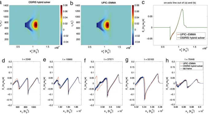
In this section, we present preliminary results of Lorentz boosted frame LWFA simulations using the hybrid solver in OSIRIS. For comparison, we performed simulations with the same param-eters using UPIC-EMMA which uses a spectral Maxwell solver.

Table 2lists the simulation parameters. We use a moving antenna in both cases to launch lasers into the plasma. The results are sum-marized inFig. 4.

InFig. 4(a)–(b) the E1field at t′

=

3955

ω

−01 for simulations

with both the hybrid solver and spectral solver in the Lorentz boosted frame are plotted, where

ω

0is the laser frequency in the

lab frame. Both the spectral solver and hybrid solver give simi-lar boosted frame results, and there is no evidence of NCI affect-ing the physics in either case. We plot the line out of the on-axis

wakefield in Fig. 4(c), which shows very good agreement with

one another. The very good agreement can also be seen when we transformed the boosted frame data back to the lab frame. In

Fig. 4(d)–(h) we plot the on-axis E1field for the OSIRIS lab frame

data, the transformed data for the OSIRIS boosted frame simula-tion with the hybrid solver, and the transformed data from the UPIC-EMMA boosted simulation at several values of time in the lab frame. As seen inFig. 4(d)–(h), the transformed data from the two boosted frame simulations agrees very well with each other.

In this paper, we mainly focus on LWFA simulations in a Lorentz boosted frame. However, it is worth pointing out that the hybrid solver can likewise be used for LWFA lab frame simulations with a moving window. When a self-injected or externally injected electron beam is accelerated by the wakefield, it will also suffer from numerical Cerenkov radiation (NCR), and may even be susceptible to the NCI in some cases. The resulting unphysical

Table 2

Parameters for a 2D LWFA simulations in the lab frame and Lorentz boosted frame that were used for in 2D Cartesian geometry with the hybrid solver in OSIRIS and with a fully spectral solver in UPIC-EMMA. The laser frequencyω0and number

k0in the lab frame are used to normalize simulation parameters. The density is normalized to the critical density in the lab frame, n0=meω20/(4πe2).

Plasma density n0 1.148×10−3_n 0γb length L 7.07×104_k−1 0 /γb Laser pulse lengthτ 70.64k−1 0 γb(1+βb) pulse waist W 117.81k−1 0 polarization _3-directionˆ

normalized vector potential a0 4.0 Lab frame simulation(γb=1)

grid size(1x1, 1x2) (0.2k −1 0 ,2.75k −1 0 ) time step1t/1x1 0.996

number of grid (moving window) 4000×512

particle shape quadratic

2D boosted frame simulation(γb=14)

grid size1x1,2 0.0982k

−1 0 γb(1+βb)

time step1t/1x1 0.125

number of grid 8192×512

particle shape quadratic

EM fields can lead to unphysical emittance growth. Applying the hybrid solver in lab frame simulations will greatly reduce the NCR, which may lead to more accurate emittance values. As a result, although not shown in this paper, we likewise benchmarked the hybrid solver with Yee solver in LWFA lab frame simulation by comparing the wakefields and laser evolution in the two cases, and very good agreement was obtained.

7. Summary

We proposed to use a hybrid Yee-FFT and a rigorous charge con-serving current deposit for solving Maxwell’s equations in order

c

b

a

d

e

f

g

h

Fig. 4. Comparison between OSIRIS lab frame, OSIRIS with the hybrid solver in the boosted frame and UPIC-EMMA in the boosted frame. In (a) and (b), 2D plots of E1for OSIRIS with the hybrid solver and UPIC-EMMA at t′₌

3955ω−1

0 are shown in the boosted frame, whereω0is the laser frequency in the lab frame. In (c), lineouts along the laser propagation direction of the same data are shown. In (d)–(h), lineouts of the E1data transformed back to the lab frame are shown. The colored lines correspond to an OSIRIS lab frame simulation, an OSIRIS hybrid solver simulation in the Lorentz boosted frame, and UPIC-EMMA simulation in the Lorentz boosted frame. (For interpretation of the references to colour in this figure legend, the reader is referred to the web version of this article.)

to eliminate the numerical Cerenkov instability in PIC codes when modeling plasmas or beams that drift with relativistic speeds in a particular direction. In this solver we solve the Maxwell’s equation in k1space along the drifting direction (x

ˆ

1direction), and use

sec-ond order finite difference representation for the derivatives in the other directions. This provides greater than Nth order accuracy for the spatial derivatives in the

ˆ

x1direction, while keeping the locality

of the field solve and current deposit in the directions transverse to1. For the current deposit, we start from the charge conserving

ˆ

deposit in OSIRIS and then correct it so that it still satisfies the con-tinuity equation for the hybrid solver. Thus, Gauss’s law remains rigorously satisfied at every time step if it is satisfied initially.

It is found from the NCI theory that such a hybrid solver has similar NCI properties in comparison to a full spectral solver that solves Maxwell equation in multi-dimensional

⃗

k space. As a result,

the

(µ, ν

1

) = (

0

,

0

)

NCI modes have a growth rate one order of

magnitude smaller than the fastest growing

(µ, ν

1

) = (

0

, ±

1

)

NCI

modes, and are highly localized. In addition, the growth rates of the

(µ, ν

1

) = (

0

,

0

)

modes decrease as one reduces the simulation

time step, and their locations in Fourier space also move farther away from the physics.

Compared with the spectral solver, the hybrid solver performs an FFT only along the drifting direction of the plasma. As a result, it saves the computation of FFT in the other directions if this ulti-mately becomes an issue for parallel scalability. In addition, it can be readily adapted into fully operational FDTD codes without the need to modify various boundary conditions in the transverse di-rections. Very importantly, this idea can be readily applied to the quasi-3D algorithm in which the quantities are decomposed into azimuthal harmonics. In this algorithm FFTs cannot be used in the

ˆ

r direction. We demonstrate the feasibility of the hybrid Yee-FFT

solver in 2D/3D Cartesian geometry, as well as in the quasi-3D ge-ometry. Although we have not conducted a rigorous theoretical analysis for the NCI in the r–z or quasi-3D geometries, we find in

simulations that the hybrid solver in quasi-3D geometry has very similar NCI properties to that in the 2D Cartesian geometry.

We show that the strategy to eliminate NCI in the hybrid solver for 2D/3D Cartesian geometry, as well as quasi-3D geometry, is similar to that for the spectral solver. The fastest growing NCI modes can be eliminated by applying a low-pass filter in the cur-rent. The

(µ, ν

1

) = (

0

,

0

)

NCI modes can be eliminated by

re-ducing the time step which both reduces their growth rates and moves them away from the physical modes in Fourier space. These NCI modes can also be fully eliminated by slightly modifying the EM dispersion relation along k1direction at the location in Fourier

space where the

(µ, ν

1

) = (

0

,

0

)

modes reside. This approach is

demonstrated in both Cartesian and quasi-3D geometry.

We showed that the new hybrid solver in OSIRIS can be used to conduct 2D LWFA simulations in a Lorentz boosted frame. With the low-pass filter applied to current and using reduced time step, we observe no evidence of NCI affecting the physics in the sim-ulation. Very good agreement is found between the results from OSIRIS with the hybrid solver, UPIC-EMMA simulations, as well as OSIRIS lab frame simulations with the standard Yee solver. This demonstrates the feasibility of using the hybrid solver to perform high fidelity relativistic plasma drift simulation.

Acknowledgments

This work was supported by US DOE under grants DE-SC0008491, DE-SC0008316, DE-FG02-92ER40727, and by the US National Science Foundation under the grant ACI 1339893, OCI 1036224, and by NSFC 11425521, 11535006, 11175102, 11375006, and Tsinghua University Initiative Scientific Research Program, and by the European Research Council (ERC-2010-AdG Grant 267841), and by LLNL’s Lawrence Fellowship. Simulations were carried out on the UCLA Hoffman2 and Dawson2 Clusters, and on Hopper Clus-ter of the National Energy Research Scientific Computing CenClus-ter, and on Blue Waters cluster at National Center for Supercomputing Applications at UIUC.

Appendix. Numerical dispersion for relativistically drifting plasma and NCI analytical expression in hybrid solver

According to Refs. [9,10], the numerical dispersion for the hybrid solver can be expressed as



(ω

′

₋

k′₁

v

0

)

2

−

ω

2 p

γ

3

(−

1

)

µSj1SE1

ω

′

[

ω]



×



[

ω]

2

− [

k

]

_E1

[

k

]

_B1

− [

k

]

_E2

[

k

]

_B2

−

ω

2 p

γ

(−

1

)

µ Sj2

(

SE2

[

ω] −

SB3

[

k

]

E1

v

0

)

ω

′

₋

_k′ 1

v

0



+

C

=

0 (A.1)

whereCis a coupling term in the dispersion relation C

=

ω

2 p

γ

(−

1

)

µ

[

ω]



Sj1SE1

ω

′

[

k

]

E2

[

k

]

B2

(v

02

−

1

)

+

Sj2SE2

[

k

]

E2

[

k

]

B2

(ω

′

−

k′1

v

0

)

+

Sj1

[

k

]

E2

(

SE2

[

k

]

B1k2

v

0

−

SB3k2

v

20

[

ω])



(A.2) and for the hybrid solver

[

k

]

_E1

= [

k

]

_B1

=

k1

[

k

]

E2

= [

k

]

B2

=

sin

(

k21x2

/

2

)

1x2

/

2

.

(A.3) We can expand

ω

′_{around the beam resonance}

_ω

′

₌

_k′

1

v

0in

Eq.(A.1), and write

ω

′

=

k′₁

v

0

+

δω

′, where

δω

′is a small term.

This leads to a cubic equation for

δω

′ _{(see [10] for the detailed} derivation), A2

δω

′3

+

B2

δω

′2

+

C2

δω

′

+

D2

=

0 (A.4) where A2

=

2

ξ

03

ξ

1 B2

=

ξ

02



ξ

2 0

− [

k

]

E1

[

k

]

B1

− [

k

]

E2

[

k

]

B2

−

ω

2 p

γ

(−

1

)

µSj2

(

SE2

ξ

1

−

ζ

1SB3′

[

k

]

E1

)



C2

=

ω

2 p

γ

(−

1

)

µ



ξ

2 0Sj2

(ζ

0SB3′

[

k

]

E1

−

SE2

ξ

0

) − ξ

1Sj1

[

k

]

E2k2SE2

[

k

]

B1

+

ξ

₀

[

k

]

_E2

(

Sj2SE2

[

k

]

B2

−

Sj1k2

ζ

1SB3′

ξ

0

)



D2

=

ω

2 p

γ

(−

1

)

µ

ξ

0

[

k

]

E2k2Sj1



SE2

[

k

]

B1

−

ζ

0SB3′

ξ

0



(A.5) where

ξ

0

=

sin

(˜

k11t

/

2

)

1t

/

2

ξ

1

=

cos

(˜

k11t

/

2

)

ζ

0

=

cos

(˜

k11t

/

2

)

ζ

1

= −

sin

(˜

k11t

/

2

)

1t

/

2

˜

k1

=

k1

+

ν

1kg1

−

µω

g

.

(A.6) We use sl,i

=



sin

(

ki1xi

/

2

)

1xi

/

2



l+1 (A.7)

as well as use the corresponding interpolation functions for the EM fields used to push the particles

SE1

=

sl,1sl,2sl,3

(−

1

)

ν1 SE2

=

sl,1sl,2sl,3 SE1

=

sl,1sl,2sl,3

SB1

=

sl,1sl,2sl,3 SB2

=

sl,1sl,2sl,3

(−

1

)

ν1

S_B3

=

s_l,1s_l,2s_l,3

(−

1

)

ν1 (A.8)

when using the momentum conserving field interpolation, and use

SE1

=

sl−1,1sl,2sl,3

(−

1

)

ν1 SE2

=

sl,1sl−1,2sl,3

SE1

=

sl,1sl,2sl−1,3

SB1

=

sl,1sl−1,2sl−1,3 SB2

=

sl−1,1sl,2sl−1,3

(−

1

)

ν1

SB3

=

sl−1,1sl−1,2sl,3

(−

1

)

ν1 (A.9)

when using the energy conserving field interpolation. The

(−

1

)

ν1 term is due to the half-grid offsets of these quantities in the1

ˆ

direction. With respect to the current interpolation,

Sj1

=

sl−1,1sl,2sl,3

(−

1

)

ν1 Sj2

=

sl,1sl−1,2sl,3

Sj3

=

sl,1sl,2sl−1,3

.

(A.10)

We note that we use expressions for charge conserving current de-position scheme that are strictly true in the limit of vanishing time step1t

→

0. The coefficients A2to D2are real, and completely

determined by k1and k2. By solving Eq.(A.4)one can rapidly scan

the NCI modes for a particular set of

(µ, ν

1

)

.

References

[1]T. Tajima, J.M. Dawson, Phys. Rev. Lett. 43 (1979) 267.

[2]S.F. Martins, R.A. Fonseca, W.B. Mori, L.O. Silva, Astrophys. J. Lett. 695 (2009) L189–L193.

[3]F. Fiuza, R.A. Fonseca, J. Tonge, W.B. Mori, L.O. Silva, Phys. Rev. Lett. 108 (2012) 235004.

[4]S.C. Wilks, W.L. Kruer, M. Tabak, A.B. Langdon, Phys. Rev. Lett. 69 (1992) 1383.

[5]J. Tonge, et al., Phys. Plasmas 16 (2009) 056311. [6]J. May, et al., Phys. Rev. E 84 (2011) 025401(R);

J. May, et al., Phys. Plasmas 21 (2014) 052703. [7]B.B. Godfrey, J. Comput. Phys. 15 (1974) 504.

[8]B.B. Godfrey, J.-L. Vay, J. Comput. Phys. 248 (2013) 33–46. [9]X. Xu, et al., Comput. Phys. Comm. 184 (2013) 2503–2514. [10]P. Yu, et al., Comput. Phys. Comm. 192 (2015) 32–47. [11]P. Yu, et al., J. Comput. Phys. 266 (2014) 124.

[12]B.B. Godfrey, J.-L. Vay, I. Haber, J. Comput. Phys. 258 (2014) 689. [13]B.B. Godfrey, J.-L. Vay, J. Comput. Phys. 267 (2014) 1.

[14]B.B. Godfrey, J.-L. Vay, I. Haber, IEEE Trans. Plasma Sci. 42 (2014) 1339. [15]K. Nagata, (Ph.D. thesis), Osaka University, 2008.

[16] P. Yu, et al., Proc. 15th Advanced Accelerator Concepts Workshop, Austin, TX, 2012, in: AIP Conf. Proc. 1507, 416 (2012).

[17]J.-L. Vay, Phys. Rev. Lett. 98 (2007) 130405.

[18]S.F. Martins, R.A. Fonseca, W. Lu, W.B. Mori, L.O. Silva, Nat. Phys. 6 (2010) 311. [19]J.-L. Vay, C.G.R. Geddes, E. Cormier-Michel, D.P. Grote, J. Comput. Phys. 230

(2011) 5908.

[20]S.F. Martins, R.A. Fonseca, L.O. Silva, W. Lu, W.B. Mori, Comput. Phys. Comm. 181 (2010) 869.

[21]B.B. Godfrey, J. Comput. Phys. 19 (1975) 58.

[22]K. Yee, IEEE Trans. Antennas and Propagation 14 (1966) 302. [23]J.M. Dawson, Rev. Modern Phys. 55 (2) (1983) 403. [24]A.T. Lin, J.M. Dawson, H. Okuda, Phys. Fluids 17 (1974) 1995. [25]J.-L. Vay, I. Haber, B.B. Godfrey, J. Comput. Phys. 243 (2013) 260.

[26]R.A. Fonseca, et al., in: P.M.A. Sloot, et al. (Eds.), ICCS, in: Lect. Notes Comput. Sci., vol. 2331, 2002, pp. 342–351.

[27]A. Lifschitz, et al., J. Comput. Phys. 228 (2009) 1803. [28]A. Davidson, et al., J. Comput. Phys. 281 (2015) 1063.

[29]P. Yu, et al., Proc. 16th Advanced Accelerator Concepts Workshop, San Jose, California, 2014.

[30]T. Esirkepov, Comput. Phys. Comm. 135 (2001) 144.

[31] I. Haber, et al. in: Proc. Sixth Conf. on Num. Sim. Plasmas, Berkeley, CA, 1973, pp. 46–48.