Active vibration control of a piezoelectric beam using PID
controller: Experimental study
Abstract
Vibration suppression of smart beams using the piezoelec-tric patch structure is presented in the present work. The smart system consists of a beam as the host structure and piezoceramic patches as the actuation and sensing elements. An experimental set-up has been developed to obtain the active vibration suppression of smart beam. The set-up con-sists of a smart cantilever beam, the data acquisition system and a LabView based controller. Experiments are performed for different beam specimen. The coupled efficient layerwise (zigzag) theory is used for theoretical finite element model-ing. The finite element model is free of shear lockmodel-ing. The beam element has two nodes with four mechanical and a vari-able number of electric degrees of freedom at each node. In the thickness direction, the electric field is approximated as piecewise linear across an arbitrary number of sub-layers in the piezoelectric layers. Cubic Hermite interpolation is used for the deflection, and linear interpolation is used for the ax-ial displacement and the shear rotation. Undamped Natural Frequencies are obtained by solving the Eigen Value prob-lem using Subspace Iteration method for cantilever beam. A state space model characterizing the dynamics of the physi-cal system is developed from experimental results using PID approach for the purpose of control law design. The exper-imental results obtained by using the active vibration con-trol system have demonstrated the validity and efficiency of PID controller. Experiments are conducted to compare the controlling of various cantilever beams of different sizes. It shows that the present actuator and sensor based control method is effective and the LabView control plots for vari-ous beams can be used as a benchmark for analytical work. The results are compared with ABAQUS software and 1D Finite element formulation based on zigzag theory.
Keywords
Zig-zag theory, LabView, 2D ABAQUS, PID controller, FEM.
Najeeb ur Rahman∗ and M. Naushad Alam
Department of Mechanical Engineering, Ali-garh Muslim University, AliAli-garh,U.P-202002, India.
Received 30 Apr 2012; In revised form 24 May 2012
∗
1 INTRODUCTION
The concept of smart or intelligent structures has started a new structural revolution. A smart structure typically consists of a host structure incorporated with sensors and actuators coor-dinated by a controller. The integrated structure system is called a smart structure because it has the ability to perform self-diagnosis and adapt to the environment change. For active vibration control, the design of piezoelectric smart structures need both the structural dynam-ics and control theories to be considered. The finite element method proved to be a powerful tool for analyzing such complex structures. The effectiveness of active control depends on the mathematical model and control strategy. Baz and Poh [3] presented a modified independent modal space control (MIMSC) method. By using this method one piezoelectric actuator can control several modes at the same time.
work out when high uncertainties on model parameters exist. Zhi-cheng et al. [4] presented the theoretical analysis and experimental results of active vibration suppression of a flexible beam with bonded discrete PZT patches sensors / actuators and mounted accelerometer.
To predict the response of laminates more accurately, many models have been developed on the basis of kinematic assumptions. In a new class of laminate theory, called the First Order Zigzag Theory (FZZT), in plane displacements in a laminate are assumed to be piece-wise (Layer-piece-wise) linear and continuous through the thickness, yet the total number of degrees of freedom is only five (doesn’t depend on the number of layers). This is accomplished by analytically satisfying the transverse shear stress continuity conditions at each interface in the laminate. This theory claims to be very accurate for many cases, especially symmetric laminates. Significant improvements have been made to the FZZT [1]. The primary improve-ment was achieved by superimposing a piecewise linear variation of in-plane displaceimprove-ments on a continuous cubic function of the transverse coordinate , creating a displacement field that can better account for the warping that occurs during bending of asymmetric laminates. Kapuria and Alam [9] have developed a novel coupled zigzag theory for linear static and dy-namic analysis of hybrid beams under electro-mechanical load which was extended to the linear static analysis of hybrid plate. Yang and Zhifei [19] presented state-space differential quadratic method (SSDQM) is extended to study the free vibration of a functionally graded piezoelectric material (FGPM) beam under different boundary conditions. The FGPM beam is approxi-mated as a multi-layered cantilever. Kapuria and Yasin [10] used layerwise plate theory and proposed the active vibration suppression of hybrid composite and fiber metal laminate (FML) plates integrated with piezoelectric fiber reinforced composite (PFRC) sensors and actuators. Zabihollah et al. [20] developed a finite element model based on the layerwise displacement theory which incorporates the electro-mechanical coupling effects. They developed an experi-mental set-up to determine the natural frequency and damping factor of the smart laminated beam and compared the results with simulation results.
The present work intends to investigate the vibration suppression of smart cantilever beams which consists of a beam as the host structure and piezoceramic patches as the actuation and sensing elements. An experimental set-up has been developed to obtain the active vibration suppression of smart beam. The experimental results are compared with 1D-FE and 2D-FE results.
2 STRUCTURAL MODELING
2.1 The coupled zig-zag beam theory approximations
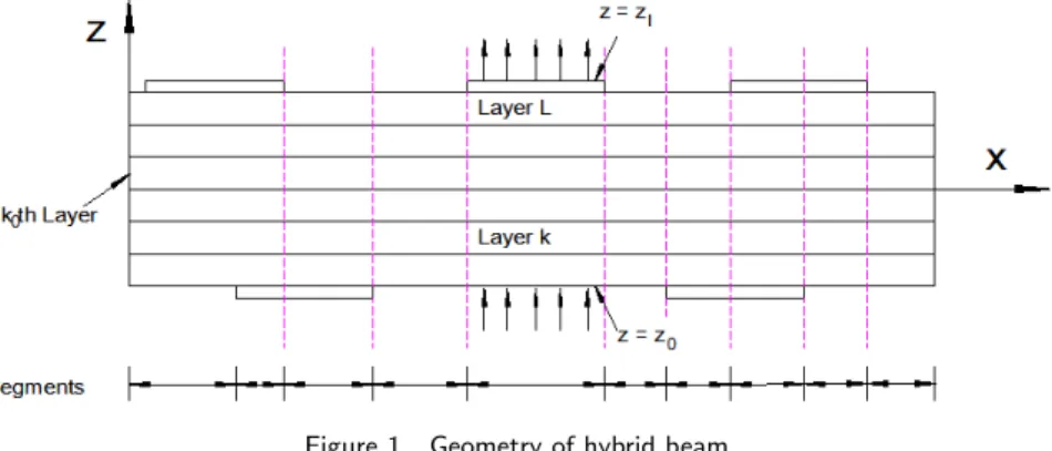
Consider a hybrid beam as shown in Fig. 1. The thickness of the beam varies segment wise due to the presence of piezoelectric patches. The bottom and top surfaces of the beam are z=z0and z=zL planes, which may vary segment-wise. All the elastic and piezoelectric layers
A state of plane stress is assumed i.e. σy=τxy=τyz =0 for a beam with a small width. A
plane strain state εy =γyz = γxy =0 is considered for infinite panels. The transverse normal
stress, σz is neglected. The axial displacement, u, transverse displacement, w and electric
potential φ are assumed to be independent of y. With these assumptions, the general 3D
constitutive equations of a piezoelectric medium for stressesσx, τzx and electric displacements
Dx, Dy reduce to
σx= Qˆ11εx− eˆ31Ez τzx= Qˆ55γzx− ˆe15Ex
Dx= eˆ15γzx+ ηˆ11Ex Dz = eˆ31εx+ ηˆ33Ez
(1)
where ˆQ11,Qˆ55; ˆe31,ˆe15;ˆη11,ηˆ33 are the reduced stiffness coefficients, piezoelectric stress
con-stants and electric permittivities.
Figure 1 Geometry of hybrid beam
The potential field φt time tis assumed as piecewise linear between nφoints zϕj across the
thickness [12]:
φ(x, z, t)= Ψjφ(z)φj(x, t) (2)
whereφj(x, t)
= φ(x, zφj, t)Ψ j
φ(z) are linear interpolation functions. The variation of
deflec-tionws obtained by integrating the constitutive equation for εz by neglecting the contribution
of σx via Poisson’s effect compared to that due to the electric field: w,z ≃ −d33φ,z ⇒
w(x, z, t)=w0(x, t)−Ψ¯jφ(z)φj(x, t) (3)
where ¯Ψjφ(z)=z∫ 0
d33Ψjφ,z(z)dz is a piecewise linear function. The axial displacement ufor the
kth layer is approximated to follow a global third order variation across the thickness with a layerwise linear variation
u(x, z, t)= u0(x, t)−zw0,x(x, t)+zψk(x, t)+z
2
ξ(x, t)+z3η(x, t) (4)
u0 and ψ0are the axial displacement and the shear rotation atz = 0, respectively. Using
shear traction-free conditionsτzx =0 at z=±h/2, the functions uk, ψk, ξ, η are expressed in
terms of u0 and ψ0 to yield
u(x, z, t)= u0(x, t)−zw0,x(x, t)+Rk(z)ψ0(x, t)+Rkj(z)φj,x(x, t) (5)
whereRkj(z), are cubic functions of z whose coefficients are dependent on the material
prop-erties and lay-up. Eqs. (5) and (3) for u, w can be expressed as
u=f1(z)u¯1w=f2(z)u¯2 (6)
With
¯
u1=[ u0 −w0,x ψ0 φj,x ] T
,u¯2=[ w0 −φj ] T
(7)
f1(z)=[ 1 z Rk(z) Rkj(z) ], f2(z)=[ 1 Ψ¯
j
φ(z) ] (8)
where elements with index j mean a sequence of elements with j = 1 to nφ. Using Eqs. (6)
and (2), the strains and the electric fields can be expressed as
εx =u,x=f1(z)ε¯1, γzx=u,z+w,x=f5(z)ε¯5.
Ex =−φ,x =−Ψjφ(z)φ j
,x(x), Ez =−φ,z =−Ψjφ(z)φ
j(x) (9)
2.2 Hamilton’s Principle
Let p1
z, p
2
z be the normal forces per unit area on the bottom and top surfaces of the beam
in direction z. Let there be distributed viscous resistance force with the distributed viscous damping coefficientc1per unit area per unit transverse velocity of the top surface of the beam.
At the interface at z = zφji where the potential is prescribed, the extraneous surface charge
density isqji. Using the notation. . .=
L
∑
k=1
z− k ∫
z+ k−1
(. . .)bdz for integration across the thickness, the extended Hamilton’s principle for the beam reduces to
∫ x ⎡⎢ ⎢⎢ ⎢⎢ ⎣
ρ u δu+ρ w δw+σxδεxτzxδγzx−DxδExDzδEz−bp1
zδw(x, z0, t) −b{p2
z−c1w˙(x, zL, t)}δw(x, zL, t)+bDz(x, z0, t)δφ 1−
bDz(x, zL, t)δφnφ
−bqjiδφji
⎤⎥ ⎥⎥ ⎥⎥ ⎦
dx
−⟨σxδu+τzxδw+Dxδφ⟩x=0
(10)
Substituting the expressions (6) and (2) for u, w, φ and (9) forεx, γzx, Ex, Ez into Eqn
(10) yields ∫ x ⎡⎢ ⎢⎢ ⎢⎣
δu¯T1Iu¯ 1
+δu¯T2I¯u¯2+δε¯T1F1+δε¯5TF5+δφj,xHj+δφjGj−(F2−Fˆ2)δw0 −(F4j−Fˆ
j
4)δφ
j
⎤⎥ ⎥⎥ ⎥⎦dx −[N¯xδu¯0+V¯xδw¯0−M¯xδw¯0,x+P¯xδψ¯0+(H¯j −V¯
j φ)δφ¯
j+S¯j xδφ
j
,x]∣x =0
where an over-bar on the stress and electric resultants and on u0, w0, ψ0, φj means values
at the ends. In this equation, I, I¯ are the inertia matrices, F1 is the stress resultant of
σx; F5, Vx, Vφj are the stress resultants of τzx andHj, GjfDx, Dz are the electric resultants
[12].
2.3 Finite element model
A two noded beam element based on the efficient layerwise zigzag theory is presented in this section. Each node has four mechanical and a variable number of electric degrees of freedom. Cubic Hermite interpolation is used for expending w0, φj in terms of the nodal values of
w0, w0,x and φj, φj,x respectively, and a linear interpolation is used for u0, ψ0
The element generalized displacement vector Ue defined as
UeT =[ ueT0 w
eT
0 ψ
eT
0 φ
eT ] (12)
The contribution Tef an element to the integral in Eq. (11) is obtained as
Te=∫a0[δuˆ
TIˆ¨
ˆ
u+δεˆTDˆεˆ−δuˆTfuφ+δuˆTCˆu˙ˆ]dx (13)
Substituting the expressions for ˆu and ˆε Te can be expressed as
Te=∫a0δU
eT [NˆTIˆNˆU¨e+NˆTCˆNˆU˙e+BˆTDˆBUˆ e−NˆTf
uφ]dx. (14)
with
Ke=∫a0Bˆ
TDˆBdx, Pˆ e
=∫a0Nˆ
Tf
uφdx.. (15)
Summing up contributions of all elements to the integral in Eq. (11), the system equation can be obtained as
MU¨+CU˙ +KU =P (16)
in whichM, C, K are assembled from the element matricesMeCe, Kend U,P are the assem-bled counterparts of Ue, Pe.the mechanical boundary conditions for beam are
Clampedend∶u0=0, w0=0, w0,x=0, ψ0=0, (17)
Free end: Nx=0, Vx=0, Mx =0, Px =0.
2.4 Dynamic Response and Modal Analysis:
⎡⎢ ⎢⎢ ⎢⎢ ⎣ Muu 0 0
0 0 0
0 0 0
⎤⎥ ⎥⎥ ⎥⎥ ⎦ ⎧ ⎪ ⎪ ⎪ ⎪ ⎨ ⎪ ⎪ ⎪ ⎪ ⎩ ¨ ¯ U ¨ Φs ¨ Φa ⎫ ⎪ ⎪ ⎪ ⎪ ⎬ ⎪ ⎪ ⎪ ⎪ ⎭ + ⎡⎢ ⎢⎢ ⎢⎢ ⎣ Cuu 0 0
0 0 0
0 0 0
⎤⎥ ⎥⎥ ⎥⎥ ⎦ ⎧ ⎪ ⎪ ⎪ ⎪ ⎨ ⎪ ⎪ ⎪ ⎪ ⎩ ˙¯ U ˙ Φs ˙ Φa ⎫ ⎪ ⎪ ⎪ ⎪ ⎬ ⎪ ⎪ ⎪ ⎪ ⎭ + ⎡⎢ ⎢⎢ ⎢⎢ ⎣ Kuu Kus Kua Ksu Kss 0 Kau
0 Kaa
⎤⎥ ⎥⎥ ⎥⎥ ⎦ ⎧ ⎪ ⎪ ⎪ ⎨ ⎪ ⎪ ⎪ ⎩ ¯ U Φs Φa ⎫ ⎪ ⎪ ⎪ ⎬ ⎪ ⎪ ⎪ ⎭ = ⎧ ⎪ ⎪ ⎪ ⎨ ⎪ ⎪ ⎪ ⎩ ¯ P 0 Qa ⎫ ⎪ ⎪ ⎪ ⎬ ⎪ ⎪ ⎪ ⎭ (18)
Where, the system vector U is partitioned into vectors of mechanical displacements ¯u, unknown output voltages φs and known input actuation voltages φa Correspondingly, P is
partitioned into vectors of mechanical loads P known electric loadsQs and unknown output
electrical loads Qa
Eq. (18) is the generalised equation of dynamics obtained through finite element model using Hamilton principle based on zig zag theory. It is used for controlling various parameters by considering different conditions. Here in this study, the output voltage. φs, for open circuit
condition, is obtained as follows:
Φs=−(Kss)−
1
KsuU .¯ (19)
Substitution of Eq. (19) into Eq. (18) yields
MuuU¨¯+CuuU˙¯+[Kuu−Kus(Kss)−1Ksu]U¯
=P¯−KuaΦa. (20)
For un-damped free vibration, the damping matrix Cuu and the right-hand side vector of
the above equation are set to zero. The resulting generalised Eigen-value problem is solved using subspace iteration method [16] to obtain the un-damped natural frequenciesω for tran-sient response, Eq. (20) is solved using Newmark direct time integration method [15]. The equation of motion for un-damped free vibration can be extracted from finite element model, for modal analysis as
MuuU¨¯+[Kuu−Kus(Kss)−1Ksu]U¯ =0 (21)
MuuU¯+KmodU¯ =0 (22)
where Kmod=[Kuu−Kus(Kss)−
1
Ksu] is the modified stiffness of the host structure due to piezoelectric effect. The solution of this equation is assumed of the form
¯
U =U0ejωtwhere j= √
−1
Substituting it in equation (22)
[Kmod−ω
2
Muu]=0 (23)
The non trivial solution of this equation exist if
∣Kmod−ω
2
Muu∣=0 (24)
The equation (24) is called the characteristic equation and its roots are called the Eigen values which give the natural frequencies of the system. Thus there are n values of natural frequencies of the system ω=diag(ω1ω2ω3. . . ωn) and ωi is theith natural frequency of the
3 PID CONTROLLER
The block diagram of a simplified PID controller in a closed loop system is shown in Fig. 2 [2, 12]. In practice the output of a PID controller is given by Eq. (25) [11, 14].
u(t)=Kp{e(t)+ 1
Ti∫ t
0
e(t)dt+T dde(t)
dt } (25)
The transfer function of of a PID controller is
Gpid(s)= U(s)
E(s) =Kp+ ki
s +Kds=Kp(1+ 1 Tis
+T ds) (26)
WhereKp= Proportional gain,Ti= integral time, andTd= derivative time. The main task
of the controller tuning is to succeed high and desirable performance characteristics using the approach of determining the PID controller parameters. In the design of PID controller for active vibration control of beam, three parameters are specified in LabView block diagram: proportional gain (Kp), integral gain (Ki), and derivative gain (Kd). The performance of the controller directly depends on these parameters. In order to obtain the desired system response, these parameters must be optimally adjusted. For this aim the optimal values ofKp,
Ki and Kd are respectively adjusted as 2.45, 1 and 1.
Figure 2 Block diagram of PID controller
The variable (e) represents the tracking error, the difference between the desired input value (R) and the actual output (Y). This error signal (e) will be sent to the PID controller, and the controller computes both the derivative and the integral of this error signal. This signal (u) 12 will be sent to the plant, and the new output (Y) will be obtained. This new output (Y) will be sent back to the sensor again to find the new error signal (e). The controller takes this new error signal and computes its derivative and it’s integral again. This process goes on and on for the closed system.
4 RESULTS AND DISCUSSIONS
4.1 Experimental and Numerical works
For the experimental and numerical evaluation, the following three cantilever beam specimens are considered:
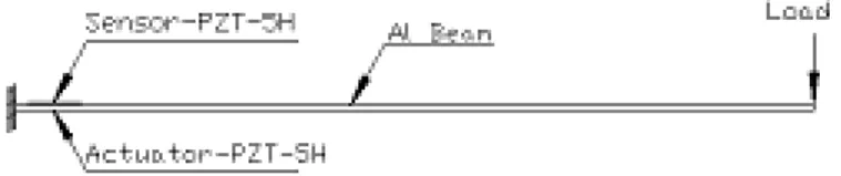
(a) An Al Beam of size 300mm×25mm×2.2mm, with a PZT-5H piezo-ceramic sensor (20mm
piezo-ceramic actuator of the same size bonded symmetrically to the bottom surface of the host beam (Fig. 3).
(b) An Al Beam of size 180mm ×27mm×2mm, with a PZT-5H piezo-ceramic sensor (15mm
× 15mm× 0.5mm) bonded to the top surface near to the fixed end and a PZT-5H
piezo-ceramic actuator (15mm ×15mm ×0.5mm) bonded symmetrically to the bottom surface
of the host beam (Fig. 4).
(c) A Composite Beam comprising of top and bottom Al layers of size 500mm×30mm×1mm
and intermediate glass fibre core of size 500mm×30mm×2mm, with a PZT-5H
piezo-ceramic sensor (50.8mm×25.4mm×0.5mm) bonded to the top surface near to the fixed
end and a PZT-5H piezo-ceramic actuator of the same size bonded symmetrically to the bottom surface of the host beam (Fig. 5).
Figure 3 Specimen Beam (a) of size 300mm×25mm×2.2mm
Figure 4 Specimen Beam (b) of size 180mm×27mm×2mm
Figure 5 Specimen Beam (c) of size 500mm×30mm×4mm
Table 1 Material properties
Elastic Properties
Material E1 E2 E3 G12 G23 G13
ν12 ν13 ν23 ρ
GPa Kg/m−3
Glass Fibre 11.04 11.04 6.75 1.57 1.53 1.53 0.12 0.32 0.32 2500
Aluminium 68 68 68 25.758 25.758 25.758 0.32 0.32 0.32 2800
PZT-5H 60.60 60.60 48.309 22.988 22.988 22.988 0.3182 0.0636 0.3182 7500
Piezoelectric Strain constants and Electric Permittivity
Material d31 d32 d33 d15 d24 e11 e22 e33
(×10−12
mV−1
) (×10−12
F m−1
)
PZT-5H -274 -274 593 741 741 3130 3130 3400
a voltage signal and inputs the signal into the computer for processing, analysis, storage, and other data manipulations. Physical phenomena represents the real world signal that we are trying to measure, such as speed, temperature, vibration, and light intensity etc. Sensors are used to evaluate the physical phenomena and produce proportionate electrical signals. Piezo-electric patch, used in the present setup, is a type of sensor that converts the beam vibration into the voltage signal that an analog to digital (A/D) converter can measure. The electrical signal produced by the sensors is fed to the controller through DAQ.
The controller inbuilt in the LabView processes the signal and gives command to DAQ device (SCB-68) to read digital input signal which converts it into an analog output signal (D/A conversion) and that output signal is fed to the piezo-actuation system. The amplified analog signal from piezo-actuation system goes to the piezo-ceramic patch known as actuator to control the beam vibration.
Figure 7 Schematic diagram of the experimental set-up
4.1.1 Experimental open-loop response
To obtain the free vibration response of the smart beam the initial tip displacement of mag-nitude 2.5 cm is applied. When the free vibrations in the beam start, the sensor deforms and due to the piezoelectric property of piezo-ceramic material, the sensor produces an electrical signal of low magnitude which is fed to the piezo-sensing system. The piezo-sensing system amplify the PZT-5H sensor signal to the voltage range of -10 to +10V with frequency range of 1-10 kHz. The piezo-sensing system output is fed to the data acquisition board consisting of A/D interface and the amplitude (voltage) vs. Time (Sec) response is obtained using LabView 8.6 (Fig.8, 9 and 10).
Figure 8 Experimental Un-control Vibration of beam (a)
Figure 9 Experimental Un-control Vibration of beam (b)
Figure 10 Experimental Un-control Vibration of beam (c)
the logarithmic decrementδas 0.0274 and the damping factorξ= 0.0658. Similarly the natural frequency, logarithmic decrement and damping factor of the other two beams are determined and listed in Table 2.
Table 2 Experimental open-loop natural frequency, logarithmic decrement and damping factor of cantilever beams
Specimen Specifications Natural Logarithmic Damping
Beam Beam Frequency (Hz) decrementδ Factor(ξ)
Beam (a) Aluminium 15.962 0.0274 0.00436
(300×3×25)mm3
Beam (b) Aluminium 24.615 0.0242 0.00385
(180×3×27)mm3
Beam (c) Composite 16.20 0.0279 0.00444
(500×5×30)mm3
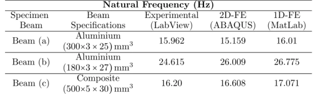
The experimental value of damping co-efficient is of great importance to design the control strategy as it directly affects the state matrices. The three experimental beams are than modeled in 2D FE (ABAQUS) and 1D FE (Matlab) and natural frequencies are obtained and validated by comparing with experimental results in Table-3. For the 2D-FE analysis, beam (a) and (c) have been modeled with 1600 eight-noded isoparametric plane stress elements for span to thickness ratio, S = 100 and beam (b) has been modeled with 1200 elements for S = 60. The results obtained using twice the above number of elements is found to be indistinguishable from these results. 1D FE results are obtained using 20 equal sized two noded elements.
Table 3 Comparison of experimental open-loop natural frequency of cantilever beams with 2D-FE and 1D-FE results.
Natural Frequency (Hz)
Specimen Beam Experimental 2D-FE 1D-FE
Beam Specifications (LabView) (ABAQUS) (MatLab)
Beam (a) Aluminium 15.962 15.159 16.01
(300×3×25)mm3
Beam (b) Aluminium 24.615 26.009 26.775
(180×3×27)mm3
Beam (c) Composite 16.20 16.608 17.071
(500×5×30)mm3
Figure 11 Mode shape of beam (a) using 2D-FE (ABAQUS)
Figure 12 Mode shape of beam (b) using 2D-FE (ABAQUS)
4.1.2 Experimental closed-loop response
To demonstrate the control strategy, the set-up utilized in section 4 has been used. A push button is simulated in the LabView to activate the controller. A 2.5 cm initial displacement has been applied at the tip of the beam and the beam is suddenly released. The sensor signal passing through the piezo-sensing system and DAQ is fed to the controller. The PID controller is configured to process the input signal from DAQ and it generates an appropriate output signal through PID algorithm. The controller response goes into DAQ (consisting of D/A interface) and the DAQ output is fed to the piezo-actuation system. The piezo-actuation system amplifies a low voltage input signal in the range of -10 to +10V to a high voltage output signal in the range of -200V to +200V and the frequency range of 1-2000Hz. The amplified signal is fed directly to the PZT-5H piezo-actuator which due to the piezoelectric properties of PZT material, produces the mechanical effect to perform closed loop control of the structure by automatic modification of the system’s structural response. Figs. (14-16) show the plots of experimental open loop vs. closed-loop response of the three beams.
Figure 14 Experimental open-loop vs. closed-loop vibration response of Beam (a)
Figure 15 Experimental open-loop vs. closed-loop Vibration response of Beam (b)
Table-Figure 16 Experimental open-loop vs. closed-loop vibration response of Beam (c)
4. On comparison of results listed in Table-2 and Table-4, it may be observed that the PID controller has maintained the natural frequency of the beams and increased the damping factor to almost double its value as in open loop response. This shows the effectiveness of LabVIEW as a controller with piezoelectric beam.
Table 4 Experimental closed-loop natural frequency, logarithmic decrement and damping factor of cantilever beams
Specimen Specifications Natural Logarithmic Damping
Beam Beam Frequency (Hz) decrementδ Factor(ξ)
Beam (a) Aluminium 15.484 0.0547 0.0087
(300×3×25)mm3
Beam (b) Aluminium 24.051 0.0377 0.0060
(180×3×27)mm3
Beam (c) Composite 16.207 0.0509 0.0081
(500×5×30)mm3
Figs. (17, 18, 19) show the amplitude-frequency response of the three beams with an extended frequency range. It is observed that the mode value of amplitude with control is lesser than the corresponding value without control at almost all frequencies. This difference in amplitude increases with increase in frequency. This shows the effectiveness of PID controller for a wider frequency range.
Figure 18 Experimental open-loop vs. closed-loop frequency response of Beam (b)
Figure 19 Experimental open-loop vs. closed-loop frequency response of Beam (c)
5 CONCLUSION
References
[1] R.C. Averill and Y.C. Yip. Thick beam theory and finite element model with zigzag approximation. AIAA J., 34:1626–32, 1996.
[2] A. Bagis. Determination of the pid controller parameters by modified genetic algorithm for improved performance.
Journal of Information Science and Engineering, 23:1469–1480, 2007.
[3] A. Baz and S. Poh. Experimental implementation of the modified independent modal space control method.Journal of sound and vibration, 139(1):133–149, 1990.
[4] Qiu Cheng-Zhi, Han Da-Jian, Zhang Min-Xian, Wang Chao-Yue, and Wu Wei-Zhen. Active vibration control of a flexible beam using a non-collocated acceleration sensor and piezoelectric patch actuator. Journal of Sound and Vibration, 326:438–455, 2009.
[5] S.B. Choi and J.W. Sohn. Chattering alleviation in vibration control of smart beam structures using piezofilm actuators, experimental verification. Journal of Sound and Vibration, 294(3):640–649, 2006.
[6] S.S Ge, T. H. Lee, G. Zhu, and F. Hong. Variable structure control of a distributed parameter flexible beam.Journal of Robotic systems, 18(1):17–27, 2001.
[7] G.Gatti, M. J. Brennan, and P. Gardonio. Active damping of a beam using a physically collocated accelerometer and piezoelectric patch actuator. Journal of Sound and Vibration, 303(3-5):798–813, 2007.
[8] G.C. Goodwin, A.R. Woodyatt, R.H. Middleton, and J. Shim. Fundamental limitations due to jω- axis zeros in siso
systems. Automatica, 35:857–63, 1999.
[9] S. Kapuria and N. Alam. Efficient layerwise finite element model for dynamic analysis of laminated piezoelectric beams.Comput. Methods Appl. Mech. Engrg, 195:2742–2760, 2006.
[10] S. Kapuria and Y. M. Yasin. Active vibration suppression of multilayered plates integrated with piezoelectric fiber reinforced composites using an efficient finite element model. J. of Sound and Vibration, 329(16):3247–3265, 2010.
[11] B.C. Kuo. Automatic Control Systems. Prentice Hall, 6th edition, 1991.
[12] W. Lianghong, W. Yaonan, Z. Shaowu, and T. Wen. Design of pid controller with incomplete derivation based on differential evolution algorithm.Journal of Systems Engineering and Electronics, 19(3):578–583, 2008.
[13] L. Meirovitch. Dynamics and Control of Structure. Wiley, New York, 1990.
[14] K. Ogata. Modern Control Engineering. Prentice Hall, 6th edition, 1997.
[15] M. Petyt. Introduction to Finite Element Variation Analysis. Cambridge University Press, Cambridge, 1990.
[16] A. Preumont.Vibration Control of Active Structures. Kluwer Academic Publishers, Dordrecht, 2004.
[17] D. Sun, J. Shan, and Y.X. Su. et al. Hybrid control of a rotational flexible beam using enhanced pd feedback with a nonlinear differentiator and pzt actuator.Smart Materials & Structures, 14(1):69–78, 2005.
[18] K. Szabat and T. Orlowska-Kowalska. Vibration suppression in a two-mass drive system using pi speed controller and additional feedbacks – comparative study. IEEE Trans Ind Electron, 54:1193–206, 2007.
[19] Li. Yang and Shi. Zhifei. Free vibration of a functionally graded piezoelectric beam via state-space based differential quadrature.Composite Structures, 87:257–264, 2009.