Universidade de Brasília
Instituto de Ciências ExatasDepartamento de Ciência da Computação
Combining Clause Learning and Resolution for
Multimodal Reasoning
Daniella Angelos
Dissertação apresentada como requisito parcial para conclusão do Mestrado em Informática
Orientadora
Prof.a Dr.a Cláudia Nalon
Brasília
2019
Universidade de Brasília
Instituto de Ciências ExatasDepartamento de Ciência da Computação
Combining Clause Learning and Resolution for
Multimodal Reasoning
Daniella Angelos
Dissertação apresentada como requisito parcial para conclusão do Mestrado em Informática
Prof.a Dr.a Cláudia Nalon (Orientadora) CIC/UnB
Prof. Dr. Bruno Lopes Vieira Prof. Dr. Thiago Paulo Faleiros
UFF CIC/UnB
Prof. Dr. Bruno Luiggi Macchiavello Espinoza
Coordenador do Programa de Pós-graduação em Informática
Dedicatória
Dedico este trabalho à minha mãe, Ilma Vitorino, por toda a dedicação e proteção dire-cionados à criação de suas filhas, que possibilitaram que eu me tornasse uma mulher forte, assim como ela. Todo o meu amor incondicional é seu, mãe. Às minhas irmãs Iasmin e Aline que viveram e vivem comigo todos os momentos, fáceis ou difíceis, também dedico este trabalho.
Dedico também ás minhas amigas de infância, Fyama e Jéssica, a família que eu escolhi. Pessoas incríveis e cheias de luz que estão ao meu lado a muitos anos. Mesmo que por vezes não encontremos tempo ou meios para nos encontrar, sempre damos um jeito de estar presente na vida uma das outras.
Por fim, dedico este trabalho ao meu melhor amigo e namorado Pedro Lima. Sua bondade, generosidade e senso de justiça me inspiram muito. Sou muito grata por ter-mos escolhido entrelaçar nossos dias com amor e carinho mútuos e pelo tanto que nos acrescentamos desde então.
Agradecimentos
Gostaria de agradeceder à professora Cláudia Nalon pela excelente orientação, sua atenção aos detalhes e seu toque humano, que fizeram total diferença ao longo de todos esses anos trabalhando juntas. Obrigada pela compreensão durante todos os meus dias difíceis. Sinto que fiz uma parceria para a vida.
Agradeço também à CAPES, a agência de fomento que subsidiou meus estudos ao longo de todo o mestrado. A bolsa que recebi foi essencial para a minha permanência na universidade.
Adiciono um agradecimento especial aos meus colegas Lucas Amaral e Felipe Rodo-poulos. Obrigada pela parceria ao longo do mestrado, os incentivos mútuos e a companhia durante os congressos.
Resumo
Vários aspectos de sistemas computacionais complexos podem ser modelados utilizando linguagens lógicas, que permitem a caracterização de noções como probabilidades, pos-sibilidades, noções temporais, conhecimento e crenças [32, 37, 38, 64]. Lógicas modais, mais especificamente, têm sido amplamente estudadas em Ciência da Computação, pois possibilitam modelar de forma natural, por exemplo, noções de conhecimento e crença em sistemas multiagentes [16, 32, 64] e aspectos temporais na verificação formal de problemas relacionados a sistemas concorrentes e distribuídos [37, 38]. Apesar de sua simplicidade, linguagens modais são expressivas para raciocinar sobre relações entre diferentes contextos ou interpretações [15].
Uma vez que um sistema é especificado em uma linguagem lógica, é possível usar mé-todos de prova para verificar as propriedades desse sistema. Em geral, se I é o conjunto de fórmulas que representam a implementação e S é o conjunto que caracteriza a especi-ficação, o processo de verificação consiste em mostrar que é possível derivar os aspectos especificados em S a partir de I. Cada método de prova corresponde a um conjunto de regras de inferência acompanhado de uma metodologia de como lidar com as fórmulas. Geralmente, a literatura sobre um sistema de prova contém análises de melhor e pior casos. Também pode-se encontrar na literatura comparações entre diferentes métodos de prova para uma linguagem lógica específica. Para lógicas modais, por exemplo, uma aná-lise empírica de desempenho de quatro sistemas de prova diferentes pode ser encontrada em [42]. Ainda é possível combinar métodos de prova para se beneficiar do melhor cenário de cada método.
Frequentemente, métodos de prova são projetados para serem implementados como provadores de teoremas automatizados, ou seja, aspectos relacionados à busca por uma prova também são considerados no projeto de um método de prova específico. Na lite-ratura, existem vários provadores de teoremas para lógicas modais [4, 67, 76, 77]. Neste trabalho, o foco é o provador de teoremas para a lógica multimodal básica Kn: KSP [61], que implementa o método baseado em resolução proposto em [60]. Kn é a linguagem que estende a lógica proposicional clássica com a adição dos operadores modais de necessidade, denotado por a , e de possibilidade, denotado por ♦a , ambos indexados por um agente a.
A semântica dos operatores é dada por “é necessário do ponto de vista do agente a” e “é possível do ponto de vista do agente a”, respectivamente.
O KSP traduz as fórmulas de entrada para uma forma normal clausal na qual cláusulas são rotuladas pelo nível modal em que ocorrem, ajudando a restringir aplicações desneces-sários das regras de inferência do cálculo que o KSP implementa. Para reduzir o espaço de busca para uma prova, vários refinamentos e estratégias de simplificação são implemen-tadas como parte do provador KSP. Para obter o melhor desempenho para uma fórmula específica, ou classe de fórmulas, é importante escolher as estratégias e otimizações mais adequadas.
De acordo com [61], o KSP apresenta um ótimo desempenho se o conjunto de símbolos proposicionais for uniformemente distribuído pelos níveis modais. No entanto, quando há um grande número de símbolos proposicionais em apenas um nível específico, a eficiência diminui. A razão é que a tradução para a forma normal usada sempre gera conjuntos satisfatíveis de cláusulas proposicionais, ou seja, cláusulas sem operadores modais. Como resolução depende da saturação do conjunto de cláusulas, isso pode custar muito tempo. Este trabalho contribui para o KSP com a implementação de uma opção adicional à lista de estratégias disponíveis do provador. O objetivo dessa nova opção é tentar reduzir o tempo que o KSP gasta saturando o conjunto de cláusulas, e, possivelmente, aumentar a velocidade na qual as regras de inferência que lidam com o raciocínio modal podem ser aplicadas. Portanto, a contribuição deste trabalho consiste, principalmente, na adição de duas novas regras ao cálculo implementado pelo KSP. Um dos resultados apresentados é a demonstração de que as regras são corretas e a adição de ambas não interfere na completude do provador.
Nossa implementação utiliza um provador de satisfatibilidade booleana baseado em aprendizagem de cláusulas conduzida por análise de conflitos (CDCL SAT solver ). O problema de satisfatibilidade booleana (SAT) é o problema de determinar se existe al-guma valoração para as variáveis de uma fórmula proposicional que torne esta fórmula verdadeira. Provadores para este problema (SAT solvers) são em geral conhecidos por serem muito eficientes. Esses provadores comumente são capazes de resolver problemas considerados difíceis, com mais de um milhão de variáveis e milhões de restrições [35]. Uma das principais razões para o amplo uso de SAT em muitas aplicações é que os CDCL SAT solvers são muito eficientes na prática [35]. A principal idéia por trás da aprendiza-gem de cláusulas implementada nesses solvers é adicionar as causas de um dado conflito, derivado de atribuições parciais de valores de verdade a símbolos proposicionais, como cláusulas aprendidas. Então essas informações são usadas para podar a árvore de busca por uma valoração satisfatível em diferentes partes.
Competições anuais também influenciaram o desenvolvimento de implementações in-teligentes e eficientes dos provadores baseados em SAT, como Chaff [56], MiniSat [73] e Glucose [5]. Essas competições permitem que muitas técnicas sejam exploradas e criam uma extensa coleção de instâncias de problemas do mundo real e problemas projetados como desafiadores, formando um grande banco referência de casos de teste [35]. Além da análise de conflitos, os provadores modernos incluem técnicas como estruturas de dados com avaliação preguiçosa, reinicializações de busca, heurísticas de ramificação controlada por conflitos e estratégias de exclusão de cláusulas [14]. Em 2005, mais especificamente, Sörensson e Een desenvolveram um provador SAT com minimização de cláusulas de con-flito, chamado MiniSat [73], que permaneceu por um tempo como o SAT solver do estado da arte. O MiniSat é um provador popular, com um desempenho surpreendente, que implementa de forma sucinta muitas heurísticas conhecidas. Ele ganhou vários prêmios na competição SAT 2005 e tem a vantagem de ser código aberto. Mantém até hoje sua importância como uma ferramenta usada como parte integrada de diferentes siste-mas [26, 27, 28, 75]. Aproveitamos os esforços teóricos e práticos que foram direcionados em melhorar a eficiência de tais provadores para ajudar a acelerar o processo de saturação dentro dos procedimentos já implementados no KSP.
Nossa implementação modifica o provador KSP para realizar uma chamada externa ao MiniSat. O provador modificado pode ser encontrado em [1]. A idéia principal por trás dessa combinação é criar uma consulta para o SAT solver contendo cláusulas especiais criadas a partir de cada nível modal. Se o provador baseado em CDCL aprender uma ou mais cláusulas pelo procedimento de análise de conflitos, adicionamos-as ao conjunto de cláusulas proposicionais da respectiva instância do KSP, pois sabemos que essas cláusulas aprendidas são consequências do conjunto que passamos ao MiniSat. Além disso, se o MiniSat concluir que o conjunto dado como entrada é insatisfatível, também aprendemos uma cláusula que, por construção, deve ser uma das premissas das regras de inferência que lidam com raciocínio modal. Aprendendo esta cláusula, nossa hipótese é que a aplicação dessas regras será possível sem que o KSP dependa da saturação do conjunto de cláusulas proposicionais.
A combinação implementada foi testada com três grandes bancos de problemas clás-sicos, LWB [11], MQBF [43, 53] e 3CNF [53], em um Ubuntu 18.04 com um processador Intel i7 e 16 GB de memória. Assim como o KSP sozinho, nossa combinação não conseguiu resolver nenhuma instância dos problemas pertecentes ao 3CNF no limite de tempo de 20 minutos. Para os demais bancos, o limite de tempo dado foi de 100 segundos. Os resul-tados experimentais de nossa implementação executando com os bancos MQBF e LWB não apresentaram, em geral, um ganho em tempo de execução, provavelmente devido à sobrecarga que inserimos com a chamada ao MiniSat.
Entretanto, nossa implementação foi capaz de avançar o KSP na resolução de entradas insatisfatíveis de uma das famílias mais difíceis do banco LWB. Essa família corresponde ao princípio da casa dos pombos estabelecido como fórmulas em Kn. Essas fórmulas são projetadas com um grande número de símbolos proposicionais distribuídos em um máximo de dois níveis modais, o que representa exatamente o cenário para o qual desejávamos me-lhorar a eficiência do KSP. O provador sozinho é capaz de resolver cinco instâncias dessa família, enquanto nossa combinação conseguiu resolver até a nona entrada. Outros pro-vadores na literatura também apresentam grande dificuldade em resolver instâncias dessa família [61]. Além disso, a execução do KSP combinado com o MiniSat para essas entra-das em particular mostrou que o uso do MiniSat permitiu uma diminuição significativa no número de inferências necessárias para que o KSP encontrasse uma prova. Isso é re-levante quando consideramos uso de memória como parâmetro de eficiência. Este último resultado indica que nossa combinação teve um impacto positivo na execução do KSP. Acreditamos que um refinamento nas mudanças implementadas no provador, buscando um meio termo entre a sobrecarga da chamada ao MiniSat e minimizar o número de inferências feitas, poderia levar a resultados ainda melhores.
Palavras-chave: lógica modal, resolução, provador baseado em SAT, aprendizagem de cláusulas, combinação de métodos de prova
Abstract
Modal logics have been widely studied in Computer Science for allowing the character-isation of complex systems that express notions in terms of knowledge, belief etc. In this work, we focus on the theorem prover for the basic multimodal language Kn: KSP, which implements a clausal resolution method. Clauses are labelled by the modal level at which they occur, helping to restrict unnecessary applications of the resolution inference rules. KSP performs well if the set of propositional symbols are uniformly distributed over the modal levels. However, when there is a high number of variables in just one particular level, the performance deteriorates. One reason is that the specific normal form we use al-ways generates satisfiable sets of propositional clauses. As resolution relies on saturation, this can be very time consuming. Our work contributes to KSP with the implementation of an additional option to the list of available strategies. This option attempts to reduce the time KSP spends during saturation, or even to increase the rate in which inference rules that deal with modal reasoning can be applied. We modified KSP to externally call MiniSat, a popular SAT solver based on clause learning. The output from MiniSat, as well as the clauses it might learn in the proof search, gives us important information about the set of clauses at each modal level. Although the proposed combination did not improve KSP performance in average, it allowed KSP to solve more instances of the ph family than before. This is one of the hardest families of the LWB benchmark, which corresponds to the pigeonhole principle established as a formula in Kn.
Keywords: modal logics, resolution, SAT solver, clause learning, combining proof meth-ods
Contents
1 Introduction 1 2 Modal Logics 4 2.1 Syntax . . . 5 2.2 Semantics . . . 8 3 Modal-Layered Resolution 13 3.1 Clausal Resolution . . . 153.2 Modal-Layered Resolution Calculus for Kn . . . 19
3.2.1 Separated Normal Form with Modal Levels . . . 19
3.2.2 Calculus . . . 22
3.2.3 KSP . . . 27
4 Satisfiability Solvers 30 4.1 The DPLL Procedure . . . 31
4.2 Conflict-Driven Clause Learning . . . 32
4.2.1 Conflict Analysis . . . 36
4.3 Modern SAT Solvers . . . 40
4.3.1 MiniSat and Glucose . . . 42
5 Combining KSP and MiniSat 45 5.1 Combining Rules . . . 46
5.1.1 Correctness Results . . . 47
5.2 Implementation . . . 48
5.3 Experimental results . . . 52
6 Conclusion and Future Work 61
List of Figures
2.1 Annotated tree for a a (p ∨ a p). . . . 8
2.2 Example of a Kripke model for Kn . . . 10
2.3 Models that satisfy ϕ of Example 2.2.2 . . . . 11
3.1 An example of derivation for the set S in Example 3.1.1 . . . 17
3.2 Derivation schemes for Example 3.1.2 . . . 18
3.3 Inference rules . . . 22
3.4 Satisfiability proof of the formula ϕ from Example 3.2.1 . . . . 26
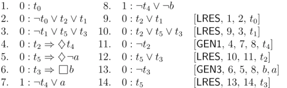
3.5 An example of a refutation . . . 27
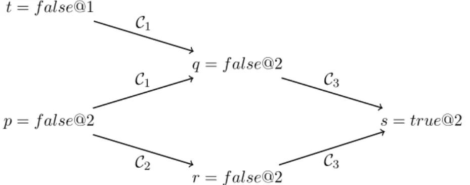
4.1 Implication graph for Example 4.2.2 . . . 34
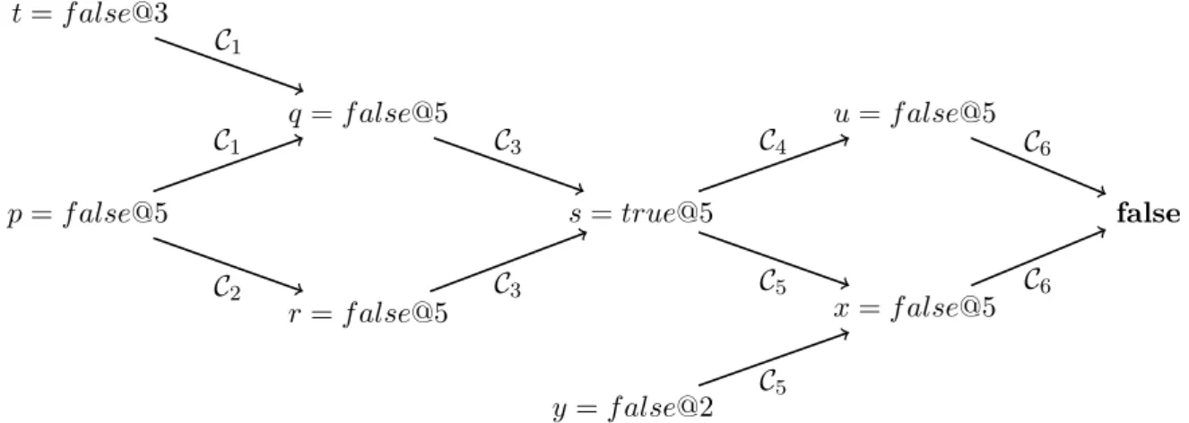
4.2 Implication graph for Example 4.2.3 . . . 35
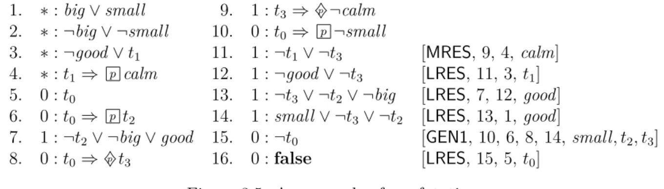
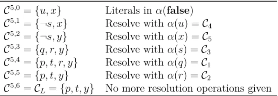
5.1 Example of refutation using KSP combined with MiniSat . . . 52
5.2 Unit resolution rules . . . 54
5.3 Benchmark results for KSP with and without the call for MiniSat . . . 57
5.4 Number of satisfiable and unsatisfiable instances solved for KSP with and without the call for MiniSat on benchmark LWB . . . 58
List of Tables
4.1 Resolution steps during clause learning . . . 38
5.1 Number of satisfiable and unsatisfiable instances solved . . . 56
5.2 Run-time in seconds for each unsatisfiable entry for family ph . . . 59
Chapter 1
Introduction
Several aspects of complex computational systems can be modelled by means of logic languages, allowing for the characterisation of notions such as probabilities, possibilities, time, knowledge and beliefs [32, 37, 38, 64]. Modal logics, more specifically, have been widely studied in Computer Science as they can naturally model, for instance, notions of knowledge and belief in multiagent systems [16, 32, 64], and temporal aspects in the formal verification of problems related to concurrent and distributed systems [37, 38]. Despite their simplicity, modal languages are expressive languages for reasoning over relations between different contexts or interpretations [15].
Once a system has been specified in a logic language, it is possible to use proof meth-ods to verify properties of such system. In general, if I is the set of formulae representing the implementation, and S is the set that characterises the specification, the verification process consists in showing that it is possible to derive the specified aspects in S from I. Each proof method corresponds to a set of inference rules accompanied with a meth-odology of how to deal with formulae. Commonly, the literature about a proof system contains descriptions of best and worst-case scenarios. We can also find in the literature comparisons between different proof methods for a specific logic language. For modal logics, for instance, an empirical performance analysis of four different proof systems can be found in [42]. It is also possible to combine proof methods in order to benefit from each method’s best-case.
Often, proof methods are designed to be implemented as an automated theorem prover, that is, aspects related to search for a proof are also addressed in the design of a particular proof method. In the literature, there are several theorem provers for modal logics [4, 67, 76, 77]. In this work, we focus on KSP [61], a theorem prover for the modal language Kn, which implements the clausal resolution method proposed in [60]. Clauses are labelled by the modal level at which they occur, helping to restrict unnecessary applications of the resolution inference rules. In order to reduce the search space for a proof, several
refinements and simplification techniques are implemented as part of KSP. To get the best performance for a particular formula, or class of formulae, it is important to choose the right strategy and optimisations.
According to [61], KSP performs well if the set of propositional symbols are uniformly distributed over the modal levels. However, when there is a high number of propositional symbols in just one particular level, the performance deteriorates. One reason is that the specific normal form used always generates satisfiable sets of propositional clauses (i.e. clauses without modal operators). As resolution relies on saturation, this can be very time consuming. Our work contributes to KSP with the implementation of an additional option to the list of available strategies. This option attempts to reduce the time KSP spends during saturation and to increase the rate in which inference rules that deal with modal reasoning can be applied.
Our implementation uses a Boolean Satisfiability Solver based on Conflict-Driven Clause Learning (CDCL), or a CDCL SAT solver. SAT solvers are well known to be very efficient in the proof search for propositional logic. They can often solve hard struc-tured problems with over a million variables and several million constraints [35]. One of the main reasons for the widespread use of SAT in many applications is that solvers based on clause learning are very effective in practice [35]. The main idea behind Conflict-Driven Clause Learning is to catch the causes of a conflict, derived from partial assignments to propositional symbols, as learned clauses, and to use this information to prune the search in a different part of the search space.
Annual competitions have also influenced the development of intelligent and efficient implementations of SAT solvers, like Chaff [56], MiniSat [73] and Glucose [5], allow-ing many techniques to be explored and creatallow-ing an extensive collection of real-world instances as well as challenging hand-crafted benchmarks problems [35]. Apart from con-flict analysis, modern solvers include techniques like lazy data structures, search restarts, conflict-driven branching heuristics and clause deletion strategies [14]. In 2005, more spe-cifically, Sörensson and Een developed a SAT solver with conflict clause minimisation, named MiniSat [73], which stayed for a while as the state-of-the-art solver. MiniSat is a popular SAT solver, with an astonishing performance, that implements many well-known heuristics in a succinct manner. It has won several prizes in the SAT 2005 competition, and has the advantage of being open-source. To this day, MiniSat keeps its importance as a tool used as an integrated part of different systems [26, 27, 28, 75]. We take advantage of the theoretical and practical efforts that have been directed in improving the efficiency of such solvers for helping to speed the saturation process within the procedures already implemented in KSP.
can be found in [1]. The main idea behind this combination is to build a query for the SAT solver containing special clauses built from each modal level. If the CDCL solver learns one or more clauses by the conflict analysis procedure, we add all them back to the set of propositional clauses of KSP, as we know that these learnt clauses are consequences of the set we passed to MiniSat. Additionally, if the solver concludes that our input is unsatisfiable, we also learn a clause that, by construction, must be one of the premises of the inference rules that deal with modal reasoning. By learning this clause, our hypothesis is that the application of these rules will be possible without KSP relying on saturation.
Although experimental results of our implementation running on classical benchmarks did not present, in general, a gain in run-time parameters, probably due to the overhead we inserted calling MiniSat, we were able to advance KSP in solving unsatisfiable entries of one of the hardest families of the LWB benchmark. This family corresponds to the pigeonhole principle established as formulae in Kn. These formulae are formatted with a large number of propositional symbols distributed over a maximum of two modal levels, which represents exactly the scenario that we wish to improve the efficiency of KSP for. The prover alone is able to solve five instances of this family while our combination managed to solve until the ninth entry. Besides, the execution of KSP combined with MiniSat for these particular entries shows that the use of MiniSat allowed an overall decrease in the number of required inferences on the search for a proof. This is noteworthy when considering both time and memory issues.
The first chapters of this work set the ground theory needed to understand the scenario in which our work fits. Chapter 2 formally introduces the syntax and semantics of the propositional modal language which is the main focus of this work: Kn. In Chapter 3 we briefly introduce clausal resolution, the base of the modal-layered calculus behind KSP. We also present the calculus KSP implements, and give an overview of how the proof search of KSP, fully presented in [61], is structured.
In Chapter 4, we discuss the basic architecture often implemented in SAT solvers, and the role of clause learning in the successful, widespread use of them. In Chapter 5 we see how we can use this solvers as a new strategy option implemented in KSP. This chapter presents the additional rules needed for the combination, as well as their soundness proofs. We also present the experimental results running KSP combined with MiniSat in Chapter 5. Finally, Chapter 6 brings a general overview of the whole work and leaves suggestions for future work.
Chapter 2
Modal Logics
This chapter formally introduces Kn, a propositional modal logic language, semantically determined by an account of necessity and possibility [58].
In classical logic, propositions or sentences are evaluated to either true or false, in any model [44]. However, in natural language, we often distinguish between various modalities of truth, such as necessarily true, known to be true, believed to be true or yet true at some
time in the future, for example.
Modal logics extend classical logic by adding operators, known as modal operators, to express one or more of these different modes of truth. Different modalities define different languages [15]. The essence in modal logics is that, in opposition to propositional logic, for instance, all the information available is not seen as from outside. Instead, the relational structure between given contexts is examined so formulae can be evaluated from inside these structures, i.e., at a particular state [15]. In this sense, the key concept behind the modal operators is to allow us to access the information held at different contexts or interpretations, an abstraction that here we may think as possible worlds.
A propositional modal language is the well known classical propositional logic language augmented by a collection of modal operators [15]. The purpose of these operators is to allow the information that holds at other worlds to be examined — but, crucially, only at worlds visible or accessible from the current one via an accessibility relation [15]. Then, the evaluation of a modal formula depends on the set of possible worlds and the accessibility relations defined over these worlds. This idea will be made precise in Section 2.2, when we define the satisfiability of formulae. It is possible to define several accessibility relations between worlds, and different modal logics are defined by restrictions on relations.
The modal language which is the focus of this work is the extension of the classical propositional logic plus the unary operators a and ♦a , whose readings are “is necessary
from the point of view of an agent a” and “is possible from the point of view of an agent
The satisfiability and validity of a formula in Kn depend on a structure known as a Kripke
model, a structure proposed by Saul Kripke to semantically analyse modal logics [46]. A
set of worlds, the accessibility relations over these worlds, and a valuation function define a Kripke model.
Kn is characterised by the schema a (ϕ ⇒ ψ) ⇒ ( a ϕ ⇒ a ψ) (axiom K), where a is an index from a finite, fixed set of agents, and ϕ, ψ are well-formed formulae as defined in Defition 2.1.1. The addition of other axioms defines different systems of modal logics and it imposes restrictions on the class of models where formulae are valid [19]. For instance, if we add the formula a ϕ ⇒ ϕ (axiom T) as an axiom, the evaluation of formulae can be restricted to models whose accessibility relations, for an agent a, are reflexive.
In the following, we will formally define the modal language. The syntax and semantics of Kn are given in Sections 2.1 and 2.2, respectively, following the presentation in [58].
2.1
Syntax
The language of Kn is equivalent to its set of well-formed formulae, denoted by WFFKn, which is constructed from a denumerable set of propositional symbols or variables P = {p, q, r, . . .}, the negation symbol ¬, the disjunction symbol ∨, the conjunction symbol ∧, the implication symbol ⇒, the double-implication symbol ⇔, and the modal connectives a and ♦a , that express the notion of necessity and possibilitiy, for each a in a finite,
non-empty fixed set of indexes A = {1, . . . , n}, where n ∈ N.
Definition 2.1.1 The set of well-formed formulae, WFFKn, is the least set such that:
1. p ∈ WFFKn, for all p ∈ P
2. if ϕ, ψ ∈ WFFKn, then so are ¬ϕ, (ϕ ∨ ψ), (ϕ ∧ ψ), (ϕ ⇒ ψ), (ϕ ⇔ ψ), ♦a ϕ and
a ϕ, for each a ∈ A
3. false, true ∈ WFFKn
We have chosen to define all connectives as primitive instead of using a minimal set of completely expressive set of connectives, as most of those connectives occur in the normal form we introduce in Section 3.2. The usual abbreviations are listed below. The logical constants false and true have the same semantic value under every interpretation. They are better known as abbreviation to the more complex formulae:
• true = ¬false (verum)
The operator ♦a is the dual of a , for each a ∈ A, that is, ♦a ϕ can also be seen as
an abbreviation for ¬ a ¬ϕ, with ϕ ∈ WFFK
n. The usual abbreviations for classical connectives are:
• ϕ ∧ ψ = ¬(¬ϕ ∨ ¬ψ) • ϕ ⇒ ψ = ¬ϕ ∨ ψ
• ϕ ⇔ ψ = (ϕ ⇒ ψ) ∧ (ψ ⇒ ϕ)
In the following, we use these abbreviations to shorten definitions as we can derive the whole set of connectives from a smaller, but still expressive, subset. The use of this subset can reduce the size of a few proofs as they rely on induction on the set of connectives. Furthermore, parentheses may be omitted if the reading is not ambiguous. Additionally, when n = 1, we may omit the index in the modal operators, i.e. we just write ϕ and
♦ϕ, for a well-formed formula ϕ.
We define a literal as a propositional symbol p ∈ P or its negation ¬p, and denote by L the set of all literals. A modal literal is a formula of the form a l or ♦a l, with l ∈ L and
a ∈ A. If l is a literal, we call ¬l its complement and say that l and ¬l form, in either
order, a complementary pair.
The modal depth of a formula is recursively defined as follows:
Definition 2.1.2 Let ϕ and ψ be well-formed formulae. We define the modal depth of a formula as mdepth : WFFKn −→ N inductively as:
1. mdepth(p) = 0, for p ∈ P
2. mdepth(¬ϕ) = mdepth(ϕ)
3. mdepth(ϕ ∨ ψ) = max{mdepth(ϕ), mdepth(ψ)}
4. mdepth( a ϕ) = mdepth(ϕ) + 1
This function represents the maximal number of nested modal operators in a formula. For instance, if ϕ = ♦p ∨ ♦q, then mdepth(ϕ) = 2.
The modal level of a formula (or a subformula), that is, the number of modal operators in the scope of which the (sub)formula occurs, is given relative to its position in an
Definition 2.1.3 Let Σ be the alphabet {1, 2, .} and Σ∗the set of all finite sequences over Σ. We define τ : WFFKn × Σ ∗ × N −→ P(WFFKn × Σ ∗ × N) as the partial function inductively defined as follows:
1. τ (p, λ, ml) = {(p, λ, ml)}
2. τ (¬ϕ, λ, ml) = {(¬ϕ, λ, ml)} ∪ τ (ϕ, λ.1, ml)
3. τ ( a ϕ, λ, ml) = {( a ϕ, λ, ml)} ∪ τ (ϕ, λ.1, ml + 1)
4. τ (ϕ ∨ ψ, λ, ml) = {(ϕ ∨ ψ, λ, ml)} ∪ τ (ϕ, λ.1, ml) ∪ τ (ψ, λ.2, ml)
with p ∈ P, λ ∈ Σ∗, ml ∈ N and ϕ, ψ ∈ WFFKn.
The function τ applied to (ϕ, 1, 0) returns the annotated syntatic tree for ϕ, where each node is uniquely identified by a subformula, its path order (or its position) in the tree, and its modal level, defined below.
Definition 2.1.4 Let ϕ be a formula and let τ (ϕ, 1, 0) be its annotated syntactic tree. We define the modal level of a subformula ϕ0 of ϕ at the position λ as mlevel : WFFKn × WFFKn × Σ∗
−→ N, and if (ϕ0, λ, ml) ∈ τ (ϕ, 1, 0) then mlevel(ϕ, ϕ0, λ) =
ml. Otherwise, it is undefined.
Example 2.1.1 If ϕ = a a (p ∨ a p), the application of τ to ϕ results in the follow-ing annotated syntatic tree, also illustrated in Figure 2.1. The nodes are rotulated by formulae, their positions are given on the left, and their modal level on the right.
τ ( a a (p ∨ a p), 1, 0) = {( a a (p ∨ a p), 1, 0), τ ( a (p ∨ a p), 1.1, 1)} = {( a a (p ∨ a p), 1, 0), ( a (p ∨ a p), 1.1, 1), (τ (p ∨ a p), 1.1.1, 2)} = {( a a (p ∨ a p), 1, 0), ( a (p ∨ a p), 1.1, 1), (p ∨ a p, 1.1.1, 2), (τ (p), 1.1.1.1, 2), (τ ( a p), 1.1.1.2, 2)} = {( a a (p ∨ a p), 1, 0), ( a (p ∨ a p), 1.1, 1), (p ∨ a p, 1.1.1, 2), (p, 1.1.1.1, 2), ( a p, 1.1.1.2, 2), (τ (p), 1.1.1.2.1, 3)} = {( a a (p ∨ a p), 1, 0), ( a (p ∨ a p), 1.1, 1), (p ∨ a p, 1.1.1, 2), (p, 1.1.1.1, 2), ( a p, 1.1.1.2, 2), (p, 1.1.1.2.1, 3)}
a a (p ∨ a p) 1 0 a (p ∨ a p) 1.1 1 p ∨ a p 1.1.1 2 p 1.1.1.1 2 1.1.1.2 a p 2 p 1.1.1.2.1 3
Figure 2.1: Annotated tree for a a (p ∨ a p).
2.2
Semantics
The semantics of Kn is presented in terms of Kripke structures.
Definition 2.2.1 A Kripke model for the set of propositional variables P and the finite set of agents A = {1, . . . , n} is given by the tuple
M= (W, R1, . . . , Rn, π)
where W is a non-empty set of possible worlds; each Ra, a ∈ A, is a binary relation on W , that is, Ra ⊆ W × W , and π : W × P −→ {false, true} is the valuation function that associates to each world w ∈ W a truth-assignment to propositional symbols.
As a remark on our notation, the truth values are written in italic (e.g. false) whereas the constants are written in bold (e.g. false).
We write Rawυ to denote that υ is accessible from w through the accessibility relation
Ra, that is (w, υ) ∈ Ra, and Ra+wυ, to mean that υ is reachable from w through a finite number of steps, that is, there exists a sequence (w1, . . . , wk) of worlds such that Rawiwi+1, for all i, 1 ≤ i < k, where w1 = w and wk = υ, with a ∈ A, w, υ, wi ∈ W and i, k ∈ N. Note that R+
a is the transitive closure of Ra, the least transitive relation that contains all elements of Ra.
Satisfiability and validity of a formula are defined in terms of the satisfiability relation.
Definition 2.2.2 Let M = (W, R1, . . . , Rn, π) be a Kripke model, w ∈ W and
ϕ, ψ ∈ WFFKn. The satisfiability relation, denoted by hM, wi |= ϕ, between a world
w and a formula ϕ, is inductively defined by:
1. hM, wi |= p if, and only if, π(w, p) = true, for p ∈ P;
2. hM, wi |= ¬ϕ if, and only if, hM, wi 6|= ϕ;
3. hM, wi |= ϕ ∨ ψ if, and only if, hM, wi |= ϕ or hM, wi |= ψ;
4. hM, wi |= a ϕ if, and only if, for all t ∈ W , (w, t) ∈ Ra implies hM, ti |= ϕ.
We can just write w |= ϕ to denote that w satisfies ϕ when the model is clear from the context. Notice that the evaluation of the a operator quantifies over all reachable worlds in the Kripke structure, characterising it as universal. The dual operator, ♦a , therefore
has an existential characterisation, forcing a world satisfying the modal literal to exist. A formula ϕ ∈ WFFKn is said to be locally satisfiable if there exists a Kripke model M = (W, R1, . . . , Rn, π) such that hM, wi |= ϕ for some w ∈ W . In this case we simply write M |=L ϕ to mean that M locally satisfies ϕ. A model M = (W, R1, . . . , Rn, π) is said to globally satisfy a formula ϕ, denoted M |=Gϕ, if for all w ∈ W , we have hM, wi |= ϕ. A formula ϕ is said to be globally satisfiable if there is a model M such that M globally satisfies ϕ. We say that a set F of formulae is locally satisfiable if the conjunction of every ϕ ∈ F is locally satisfiable. Global satisfiability of sets is defined analogously. A formula is said to be valid if it is satisfiable in all models.
The local satisfiability problem for Kn corresponds to determining the existence of a model in which a formula is locally satisfied, while the global satisfiability problem corresponds to determining the existence of a model in which a formula is globally satisfied.
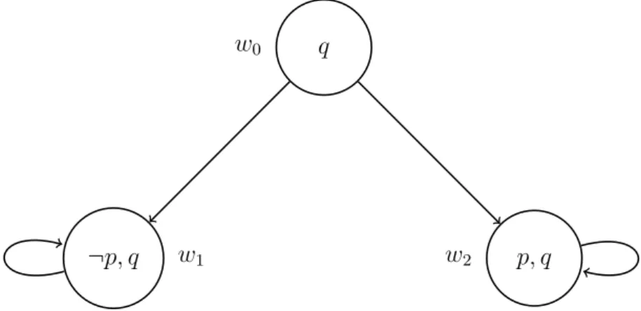
Example 2.2.1 Let M be the model illustrated in Figure 2.2. Take M = (W, R, π), for
p, q ∈ P and A = {1}, where (i) W = {w0, w1, w2} (ii) R = {(w1, w1), (w2, w2), (w0, w1), (w0, w2)} (iii) π(w, p) = true if w = w1 false otherwise
Note that w0 satisfies both ♦p and ♦¬p in M. This is a rather simple example to illustrate that, even though some sentence evaluates to true at some world, one can see the same sentence occurring with the opposite valuation through an accessibility relation. This kind of reasoning is not possible in classical propositional logic. Other examples of formulae satisfied by this model at w0 are: q ∨ p and ♦ p ∧ ♦ ¬p. Also note that q is globally satisfied in M since it is true at every world of the model.
q w0
p, q w2
¬p, q w1
Figure 2.2: Example of a Kripke model for Kn
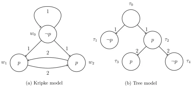
Example 2.2.2 (Tree-like model) Consider the formula ϕ = 1 (p ⇒ ♦2 p). The Figure 2.3
contains two examples of models, Figure 2.3a and Figure 2.3b, that satisfy ϕ at w0 and
τ0, respectively, hence, ϕ is locally satisfiable. Note that the model from the Figure 2.3b has a graphical representation equivalent to a tree.
As trees play an important role in future definitions, we will take this opportunity to define them formally. By a tree T we mean a relational structure (T, S) where T is a set of nodes and S is a binary relation over these nodes. T contains a unique node r0 ∈ T (called the root) such that all other nodes in T are reachable from r0, that is, for all t ∈ T , we have S+r0t. Also, every element of T , distinct from r0, has a unique S-predecessor, and S is acyclic, that is, for all t ∈ T , it is not the case that S+tt [3].
Figure 2.3b is a tree model. By a tree model we mean a Kripke model (W, R, π), with A = {1}, where (W, R) is a tree with a distinguish world w0 ∈ W as its root. A tree-like
model for Kn is a model (W, R1, . . . , Rn, π), with A = {1, . . . , n}, such that (W, ∪i∈ARi) is a tree, with w0 ∈ W as the root.
Let M = (W, R1, . . . , Ra, π) be a tree-like model for Kn with w0 ∈ W as a root. We define the depth : W −→ N of a world w ∈ W , as the length of the path from w0 to
w through the union of the relations in M. We sometimes say depth of M to mean the
longest path from the root to any world in W .
¬p w0 p w2 p w1 1 1 2 2 1
(a) Kripke model
τ0 ¬p τ1 p τ2 p τ3 ¬p τ4 1 1 2 2 (b) Tree model
Figure 2.3: Models that satisfy ϕ of Example 2.2.2
Theorem 2.2.1. Let ϕ ∈ WFFKn be a formula and M = (W, R1, . . . , Rn, π) be a model.
Then M |=L ϕ if and only if there is a tree-like model M0 such that M0 |=Lϕ. Moreover, M0 is finite and its depth is bounded by mdepth(ϕ).
The proof of Theorem 2.2.1 presented in [15] constructs a tree-like model M0 as a
generated submodel of M, that is, it restricts both the set of worlds and the binary
relations to a subset of W which is relevant to determining the satisfiability of a given formula. Then, using the satisfiability invariance of generated submodels, also proved in [15], which states that a formula is satisfiable in a model if, and only if, it is satisfiable in its generated submodels, the proof becomes trivial.
Theorem 2.2.2. Let ϕ, ϕ0 ∈ WFFKn and M = (W, R1, . . . , Rn, π) be a tree-like model
such that M |=L ϕ. If (ϕ0, λ0, ml) ∈ τ (ϕ, 1, 0) and ϕ0 is satisfied in M, then there is
w ∈ W , with depth(w) = ml, such that hM, wi |= ϕ0. Moreover, the subtree rooted at w has height equal to mdepth(ϕ0).
The proof of Theorem 2.2.2 is by induction on the structure of the formula and shows that a subformula ϕ0 of ϕ is satisfied at a node with distance ml of the root of the tree-like model. As determining the satisfiability of a formula ϕ depends only on its subformulae
ϕ0, only the subtrees of height mdepth(ϕ0) starting at level ml need to be checked. The bound on the height of the subtrees follows from Theorem 2.2.1 [60].
The global satisfiability problem for a modal logic is equivalent to the local satisfiability problem of the logic obtained by adding the universal modality, ∗ , to the original modal language [36]. Let K∗n be the logic obtained by adding ∗ to Kn. A model M∗ for K∗n is the pair (M, R∗), where M = (W, R1, . . . , Rn, π) is a tree-like model for Kn and
R∗ = W × W . A formula ∗ ϕ is satisfied at the world w ∈ W , in the model M∗, written hM∗, wi |= ∗ ϕ, if, and only if, for all w0 such that (w, w0) ∈ R∗, we have that hM∗, w0i |= ϕ. As the relation R
∗ is total, it is easy to see that this corresponds to the global satisfiability problem as defined before. In [36], the following result is established and proved, for first-order definable modal logics.
Theorem 2.2.3. M |=Gϕ, if, and only if, M∗ |=L ∗ ϕ, for a formula ϕ.
The satisfiability problems for Kn are proven to be PSPACE-complete [74], for local satisfiability, and EXPTIME-complete, for global satisfiability [74]. These might seem as discouraging results and one may wonder whether automated computation for such logics can be viable in practice. However, the kinds of formulae that give rise to the worst case scenarios seem to be hardly encountered in real applications [41]. This has allowed for the successful utilisation of modal logics in, for instance, multiagent systems [16, 32, 64] and distributed systems [37, 38], due to the implementation of automated reasoning systems that perform very well for these logics.
Chapter 3
Modal-Layered Resolution
Modal languages, in general, can be used in Computer Science to represent properties of complex systems. Once a system is described by a logical language, we also want to reason about its properties and we do this through a proof method, also called proof system or
calculus. This chapter formally introduces a calculus for the modal language defined on
Chapter 2. But first, we will go through some basic notions about proof systems.
The proof of theorems, or the deduction of consequences from assumptions, in Math-ematics, is typically characterised by a conclusion that follows from a (possibly empty) set of formulae [44].
Formally, a proof is a finite object built in conformity to a fixed set of syntactic rules [33]. The set of syntactic rules that define proofs, called inference rules, are said to specify a proof system. These rules allow the derivation of formulae from sets of formulae through strict symbol manipulation [31]. Besides the set of syntactic rules, a proof method may also be characterised by a set of statements that are assumed to be true, called axioms. Axioms may serve as premises or starting points for further reasoning. A proof system for a particular logic is said to be sound if any formula that has a proof is a valid formula of the logic, and it is complete for a particular logic if any valid formula has a proof [33]. Therefore, a sound and complete calculus allows us to produce a proof for a formula if and only if this formula is valid.
There are many kinds of proof systems. One way of categorising proof systems involves the chaining in which the rules are applied to form a line of reasoning. If the chaining starts from a set of conditions and moves toward some (possibly remote) conclusion, the system is called forward chaining. Backward systems, on the other hand, start from what is needed to be proved and moves towards the axioms. Proof search by backward chaining is a standard technique in automated reasoning [39].
One of the most common examples of a backward system is a tableau system. Tableau systems exist in many varieties and for several logics, but they all share a few aspects [33].
For example, they are all refutational systems, i.e., to prove a formula, we begin by negating it, then analysing the consequences of doing so. If it is the case that all the consequences turn out to be contradictory, we conclude that the original formula has been proved [33]. Refutational systems are based on the fact that a formula is valid if, and only if, its negation is unsatisfiable.
Other aspect common to tableau systems is that they are analytic, that is, they usually perform the search for a proof trough breaking down (or branching) the initial formula, according to certain inference rules, until a rule for closing each branch is used. Hence, proofs in tableau systems in general have a graphical representation similar to a tree [23]. Each branch of a tableau proof can be considered to be a partial description of a model on the respective logic. A tableau proof system for modal logics usually labels every step of the proof with a prefix that names a possible world1 in a model [33]. Therefore, to deal with modal reasoning, whenever a formula ♦aϕ holds in a specific world labelled by
a prefix, the tableau proof creates a new world, whose accessibility from the previous one is made explicit trough the new prefix, that satisfies the formula ϕ in the scope of the modal operator. Then, following closely the semantics of the a operator, if a ϕ0 has the same prefix of ♦aϕ, the formula ϕ0 is propagated to the newly created world. Whenever
we insert a contradiction in any world, we close the respective branch. If all branches happen to be closed, we can conclude that the original negated formula is unsatisfiable, hence, the original formula is valid.
Aside from tableaux, backward systems may also take the form of a version of Robin-son’s resolution rule [39]. Calculi based on this rule are often referred as resolution based
systems. These are also refutational systems.
Numerous resolution based systems for propositional logic have been proposed in the literature [10]. The standard system has only one inference rule [66], showed below as the RES rule, which takes two clauses with literals that form a complementary pair and generates a resolvent, where each clause, denoted by C, is a disjunction of literals. The resolution rule takes, then, the form:
[RES] Ci∨ l ¬l ∨ Cj Ci∨ Cj
where Ci and Cj are (possibly empty) clauses, called parent clauses, l is a literal and Ci∨ Cj is the resolvent.
1Here, we regard a world as a set of formulae, following the correspondence given by the syntactic
construction of a tableau proof and the construction of a model, as given in the completeness proofs for such proof methods.
We use the constant false to denote the empty clause, i.e., the clause that contains no literals. Due to the associativity and commutativity properties of disjunction, one may see a clause as a set of literals. In this work we might abuse of set notation, writing l ∈ C, when l is a literal of C, and Ci ⊆ Cj, when all literals in Ci are also literals in Cj.
Resolution-based provers are widely implemented and tested [10]. Besides reliable implementations of the main mechanism for propositional logic, presented in Section 3.1, we can also profit from several complete strategies. For instance, linear resolution [45, 50],
set of support strategy [78], ordered resolution [65] and selection-based resolution [45]. All
those strategies restrict the clauses that can be chosen as premises for the application of the resolution rule whilst retaining completeness. In other words, those strategies try to avoid unnecessary applications of the rule in order to find a proof. Provers for multimodal logics can take advantage of such strategies, as they require pruning of the search space for a proof, in order to deal with the inherent intractability of the satisfiability problem for such logics.
The proof method we will discuss in this chapter is a resolution-based calculus, it was proposed in [60] for both local and global reasoning, and it is thoroughly presented in Section 3.2. The calculus is proved to be sound and complete for Kn in [60]. It was developed with special concerning towards computer implementations and it uses formulae translated into a special normal form. This normal form divides the clause set according to the modal level at which each clause occurs to prevent unecessary applications of inference rules.
3.1
Clausal Resolution
Resolution appeared in the early 1960’s through investigations on performance improve-ments of refutational systems based on the Herbrand’s Theorem, which allows a kind of reduction of first-order logic to propositional logic [18]. J. A. Robinson incorporated the concept of unification on demand on a refutational system, creating what is now known as the resolution method for first-order logic [66].
Clausal resolution is a simple and adaptable proof system for classical logics. It was claimed to be suitable to be performed by a computer, as, for propositional logic, it has only one inference rule that is applied to the set of clauses. Robinson emphasises that, from the theoretical point of view, an inference rule need only to be sound and effective, that is, it allows only valid consequences to be deduced from premises and it must be algorithmically decidable whether an alleged application of the rule is indeed an application of it.
The single inference rule of this system of logic, the RES rule, entails the resolution
principle, namely: From any two clauses Ci and Cj which contain a complementary pair
of literals, one may infer a resolvent of Ci and Cj [66].
Resolution, as proposed by Robinson, is a refutationally complete theorem proving method for first-order logic [66]. In his paper, Robinson presents a formalisation of the calculus for first-order logic, designed to be used as the basic theoretical instrument of the proposed computer theorem-proving program. For the purpose of this work, we are only interested in the calculus for propositional logic. Therefore, we will neither discuss the theory behind the Herbrand’s Theorem nor the definition of the unification procedure, but, if curious, the reader can refer to [66] for more details. In the sense of this last remark, the only representational formalism needed is propositional logic.
Resolution relies on saturation. A clause set is said to be saturated when further relevant information cannot be generated, regardless of the rule (or set of rules) that is applied [25]. That means that the application of any rule to a saturated set of clauses only generates tautologies or repeated clauses. Saturation, up to redundancy, of the initial clause set is a quite useful criterion when we are thinking in terms of the termination proof and completeness proof of a calculus [33].
As resolution has only the RES rule, to show that a formula ϕ is valid, ¬ϕ is translated into a normal form, then the inference rule is applied until either no new resolvents can be generated or the empty clause is obtained [10]. The contradiction implies that ¬ϕ is unsatisfiable and hence, that ϕ is valid.
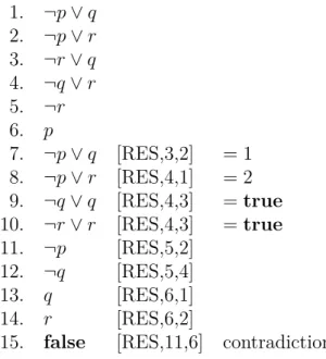
Example 3.1.1 Consider the set of clauses S = {(¬p∨q), (¬p∨r), (¬r∨q), (¬q∨r), ¬r, p}. Figure 3.1, taken from [57], shows an example of naive derivation of the empty clause for S, proving that this set is unsatisfiable.
Despite its simplicity, naive resolution is hard to implement efficiently due to the diffi-culty of finding good choices of clauses to resolve [35]. As one can infer from this example, a raw implementation of resolution-based systems typically implies considerable storage requirements. Even with such a short set of clauses (only 6 initially), the application of the resolution rule, without any restriction, yields the generation of repeated clauses, Clauses 7 and 8, and tautologies, Clauses 9 and 10. That is, useless information is generated and possibly stored until the contradiction can be found.
Robinson established two principles, namely purity principle and subsumption
prin-ciple, to discuss the development of efficient resolution systems. Such principles are called search principles in [66]. A third principle, named replacement principle, is presented in
1. ¬p ∨ q 2. ¬p ∨ r 3. ¬r ∨ q 4. ¬q ∨ r 5. ¬r 6. p 7. ¬p ∨ q [RES,3,2] = 1 8. ¬p ∨ r [RES,4,1] = 2 9. ¬q ∨ q [RES,4,3] = true 10. ¬r ∨ r [RES,4,3] = true 11. ¬p [RES,5,2] 12. ¬q [RES,5,4] 13. q [RES,6,1] 14. r [RES,6,2]
15. false [RES,11,6] contradiction
Figure 3.1: An example of derivation for the set S in Example 3.1.1
terms of replacement using the subsumption principle.
Definition 3.1.1 If S is any finite set of clauses, C is a clause in S and l a literal in C with the property that no literal in any other clause in S form a complementary pair with l, then l is said to be pure in S.
The purity principle is then based on Theorem 3.1.1.
Theorem 3.1.1. If S is any finite set of clauses, and a clause C ∈ S contains a literal l
which occurs pure in S, then S is satisfiable if and only if S \ {C} is satisfiable.
Definition 3.1.2 If Ci and Cj are two distinct nonempty clauses, we say that Ci
subsumes Cj in the case that Ci ⊆ Cj.
Theorem 3.1.2 establishes the basic property of subsumption.
Theorem 3.1.2. If S is any finite set of clauses, and Cj is any clause in S which is
subsumed by some clause in S \ {Cj}, then S is satisfiable if and only if S \ {Cj} is
satisfiable.
Theorems 3.1.1 and 3.1.2 are both proved in [66].
Another specially useful search principle derives from the subsumption principle. Sup-pose that a resolvent CR of Ci and Cj subsumes Ci. Then, in adding CR as a result of resolving Ci and Cj, we may simultaneously remove, by the subsumption principle, Ci.
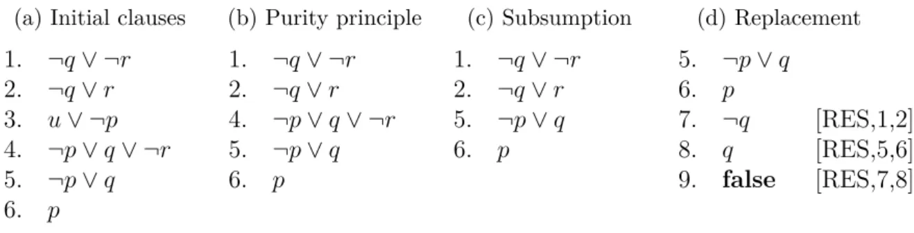
(a) Initial clauses 1. ¬q ∨ ¬r 2. ¬q ∨ r 3. u ∨ ¬p 4. ¬p ∨ q ∨ ¬r 5. ¬p ∨ q 6. p (b) Purity principle 1. ¬q ∨ ¬r 2. ¬q ∨ r 4. ¬p ∨ q ∨ ¬r 5. ¬p ∨ q 6. p (c) Subsumption 1. ¬q ∨ ¬r 2. ¬q ∨ r 5. ¬p ∨ q 6. p (d) Replacement 5. ¬p ∨ q 6. p 7. ¬q [RES,1,2] 8. q [RES,5,6] 9. false [RES,7,8]
Figure 3.2: Derivation schemes for Example 3.1.2
This combined operation leads to the replacement of Ci by CR. Accordingly, this principle is named as the replacement principle [66].
The application, to a finite set S of clauses, of any of the three search principles de-scribed, produces a set S0 which either has fewer clauses than S, or has one or more shorter clauses [66]. An evident way of profit from these principles in a refutation procedure is therefore to delay the application of the RES rule to the set of clauses, until the search principles are no longer fulfilled.
Example 3.1.2 Let S be the set of clauses showed in Figure 3.2a. This time, prior to the exaustive application of the RES rule, let’s investigate opportunities to apply the search principles, in order to reduce the number and size of clauses.
In this example, the third clause can be eliminated from the set of clauses through an application of the purity principle, as expressed in Figure 3.2b, because there is no other clause that has the complementary pair of the literal u. Furthermore, as the Clause 5 subsumes the Clause 4, this last one can also be eliminated from the set of clauses, leaving only the clauses in Figure 3.2c. The application of RES to Clauses 1 and 2 generates the resolvent ¬q, which subsumes both clauses, hence, by the replacement principle, both may be replaced by Clause 7, as showed in Figure 3.2d. Finally, the application of RES to Clauses 5 and 6, generates the Clause 8 as a resolvent, and then resolving this one with the Clause 7 will generate the empty clause, a contradiction.
There are further principles of the same general sort, possibly less simple than the ones presented earlier, which Robinson considers to be merely a brief view of the possible approaches to the efficiency problem of resolution systems. Details can be found in [66]. Further on this work, we see a practical application for the purity principle, but we refer to it as pure literal elimination following more recent literature. We also present unit
propagation, which can be thought as another search principle. Both will be brought back
3.2
Modal-Layered Resolution Calculus for
K
nWith the resolution ground for propositional logic all set, now we will present a resolution-based proof system for Kn, the modal language discussed in Chapter 2.
The calculus presented in this section requires a translation into a more expressive modal language, presented in Section 3.2.1, where labels are used to express semantic properties of a formula. This calculus uses labelled resolution in order to avoid unnecessary applications of the inference rules [60]. For instance, we do not apply resolution to clauses at different modal levels, since, as we have seen, they are not, in fact, contradictory.
3.2.1
Separated Normal Form with Modal Levels
Formulae translated into a normal form have a specific, normalised structure, possibly resulting in less operators to handle with, which may imply in a smaller number of rules for a proof system. Hence, a calculus that is planned to be implemented in a computer may take great advantage of normal forms, since the smaller number of inference rules reduces the chances of implementation errors, for example.
The normal form used in this work for Kn is a layered normal form called Separated
Normal Form with Modal Levels, denoted by SNFml, proposed in [60], hence, all the definitions in this section are adapted from [60]. A formula in SNFml is a conjunction of clauses where the modal level in which they occur is made explicit in the syntax as a label.
We write ml : ϕ to denote that ϕ occurs at modal level ml ∈ N ∪ {∗}. By ∗ : ϕ we mean that ϕ is true at all modal levels. Formally, let WFFmlKn denote the set of formulae with the modal level annotation, ml : ϕ, such that ml ∈ N ∪ {∗} and ϕ ∈ WFFKn. Let M∗ = (W, w0, R1, . . . , Rn, R∗, π) be a tree-like model and take ϕ ∈ WFFKn.
Definition 3.2.1 Satisfiability of labelled formulae is given by:
1. M∗ |=L ml : ϕ if, and only if, for all worlds w ∈ W such that depth(w) = ml, we have hM∗, wi |= ϕ;
2. M∗ |=L∗ : ϕ if, and only if, M∗ |= ∗ ϕ.
Clauses in SNFml are defined as follows.
Definition 3.2.2 Clauses in SNFml are in one of the following forms:
1. Literal clause ml :Wr i=1li
2. Positive a-clause ml : l ⇒ a m
3. Negative a-clause ml : l ⇒ ♦a m
where r, i ∈ N, ml ∈ N ∪ {∗}, l, li, m ∈ L and a ∈ A = {1, . . . , n}.
Positive and negative a-clauses are together known as modal a-clauses. The index a can be omitted if it is clear from the context.
Definition 3.2.3 Let ϕ ∈ WFFKn. We say that ϕ is in Negation Normal Form (NNF) if it contains only the operators ¬, ∨, ∧, a and ♦a. Also, only propositions
are allowed in the scope of negations.
The transformation of a formula ϕ ∈ WFFKn into SNFml is achieved by first trans-forming ϕ into its Negation Normal Form, and then, recursively applying rewriting and renaming of complex formulae [63], until all subformulae are written in one of the forms presented by Definition 3.2.2.
Formally, let ϕ be a formula in NNF. Take t as a propositional symbol not occurring in ϕ. The translation of ϕ into SNFml is then given by 0 : t ∧ ρ(0 : t ⇒ ϕ) for local satisfiability — for global satisfiability, the translation is given by ∗ : t ∧ ρ(∗ : t ⇒ ϕ) — where ρ is the translation function defined by Definition 3.2.4. We refer as initial clauses the literals clauses at the modal level 0.
Definition 3.2.4 The translation function ρ : WFFmlK
n −→ WFF ml Kn is defined as follows: ρ(ml : t ⇒ ϕ ∧ ψ) = ρ(ml : t ⇒ ϕ) ∧ ρ(ml : t ⇒ ψ) ρ(ml : t ⇒ a ϕ) = (ml : t ⇒ a ϕ), if ϕ is a literal = (ml : t ⇒ a t0) ∧ ρ(ml + 1 : t0 ⇒ ϕ), otherwise ρ(ml : t ⇒ ♦a ϕ) = (ml : t ⇒ ♦a ϕ), if ϕ is a literal = (ml : t ⇒ ♦a t0) ∧ ρ(ml + 1 : t0 ⇒ ϕ), otherwise ρ(ml : t ⇒ ϕ ∨ ψ) = (ml : ¬t ∨ ϕ ∨ ψ), if ϕ ∨ ψ is a disjunction of literals = ρ(ml : t ⇒ ϕ ∨ t0) ∧ ρ(ml : t0 ⇒ ψ), if ψ is not a a disjunction of literals
Where t, t0 ∈ L, ϕ, ψ ∈ WFFKn, a ∈ A and ml ∈ N ∪ {∗}, with ∗ + 1 = ∗. Also, whenever t0 renames a subformula ϕ, it is required that t0 is a new propositional symbol (i.e. it does not occur in the original formula).
As the conjunction operator is commutative, associative and idempotent, we will com-monly refer to a formula in SNFml as a set of clauses.
Example 3.2.1 Let ϕ be the formula (a ⇒ b) ⇒ ( a ⇒ b). We show how to
translate ϕ into its normal form, considering the local satisfiability problem. First, we anchor the NNF of ϕ to the initial state:
0 : t0∧ ρ(0 : t0 ⇒ ♦(a ∧ ¬b) ∨ ♦¬a ∨ b) (3.1) The Equation 3.1 is used to anchor the meaning of ϕ to the initial state, where the formula is evaluated. The function ρ proceeds with the translation, replacing complex formulae inside the scope of the and ♦ operators, by means of renaming.
So the translation proceeds as follows:
ρ(0 : t0 ⇒ ♦(a ∧ ¬b) ∨ ♦¬a ∨ b) = ρ(0 : t0 ⇒ ♦(a ∧ ¬b) ∨ t1) ∧ ρ(0 : t1 ⇒ ♦¬a ∨ b) = ρ(0 : t0 ⇒ t2 ∨ t1) ∧ ρ(0 : t2 ⇒ ♦(a ∧ ¬b)) ∧ ρ(0 : t1 ⇒ ♦¬a ∨ t3) ∧ ρ(0 : t3 ⇒ b) = (0 : ¬t0∨ t2 ∨ t1) ∧ (0 : t2 ⇒ ♦t4) ∧ ρ(1 : t4 ⇒ a ∧ ¬b) ∧ ρ(0 : t1 ⇒ t5∨ t3)∧ (0 : t5 ⇒ ♦¬a) ∧ (0 : t3 ⇒ b) = (0 : ¬t0∨ t2 ∨ t1) ∧ (0 : t2 ⇒ ♦t4) ∧ ρ(1 : t4 ⇒ a) ∧ ρ(1 : t4 ⇒ ¬b)∧ (0 : ¬t1∨ t5∨ t3) ∧ (0 : t5 ⇒ ♦¬a) ∧ (0 : t3 ⇒ b) = (0 : ¬t0∨ t2 ∨ t1) ∧ (0 : t2 ⇒ ♦t4) ∧ (1 : ¬t4∨ a) ∧ (1 : ¬t4 ∨ ¬b)∧ (0 : ¬t1∨ t5∨ t3) ∧ (0 : t5 ⇒ ♦¬a) ∧ (0 : t3 ⇒ b)
The translation generates eight clauses, two of them at the subsequent modal level (1 : ¬t4 ∨ a and 1 : ¬t4 ∨ ¬b). Note that, from the six clauses at the initial modal level, we have three literal clauses (0 : t0, 0 : ¬t0 ∨ t2∨ t1 and 0 : ¬t1∨ t5∨ t3), known as the initial clauses, two negative clauses (0 : t2 ⇒ ♦t4 and 0 : t5 ⇒ ♦¬a) and one positive clause (0 : t3 ⇒ b).
The set of clauses obtained by translating the formula ϕ into SNFmlis locally satisfiable if, and only if, ϕ is locally satisfiable, as given by the next lemma, taken from [60].
Lemma 3.2.1. Let ϕ ∈ WFFKn be a formula and let t be a propositional symbol not occurring in ϕ. Then:
(i) ϕ is locally satisfiable if, and only if, 0 : t ∧ ρ(0 : t ⇒ ϕ) is satisfiable;
3.2.2
Calculus
The motivation for the use of the labelled clausal normal form in the calculus is that inference rules can then be guided by the syntactic information given by the labels and applied to smaller sets of clauses, reducing the number of unnecessary applications of the inference rules, and therefore improving the efficiency of the proof procedure [61].
The modal-layered resolution calculus, proposed in [60], comprises a set of inference rules, individually explained below, for dealing with propositional and modal reasoning.
We denote by σ the result of unifying the labels in the premises for each rule. Formally presented in Definition 3.2.5, the unification function imposes restrictions on the applic-ation of the inference rules. We have seen, for instance, that contradictory clauses at different modal levels are not contradictory. Hence, a resolvent should not be deduced.
Definition 3.2.5 Unification is given by a function σ :P(N ∪ {∗}) −→ N ∪ {∗}, where σ({ml, ∗}) = ml and σ({ml}) = ml. Otherwise, σ is undefined.
The inference rules showed in Figure 3.3 can only be applied if the unification of their labels is defined (where ∗ − 1 = ∗). Note that for GEN1 and GEN3, if the modal clauses occur at the modal level ml, then the literal clause occurs at the next modal level, ml + 1. The rules that deal with modal reasoning are applied only to clauses with modal operators indexed by the same agent.
[LRES] ml1: D ∨ l ml2: D0∨ ¬l σ({ml1, ml2}) : D ∨ D0 [MRES] ml1: l1⇒ am ml2: l2⇒♦a¬m σ({ml1, ml2}) : ¬l1∨ ¬l2 [GEN2] ml1: l1⇒ am1 ml2: l2⇒ a¬m1 ml3: l3⇒♦am2 σ({ml1, ml2, ml3}) : ¬l1∨ ¬l2∨ ¬l3 [GEN1] ml1: l1⇒ a¬m1 .. . mlr: lr⇒ a¬mr mlr+1: l ⇒♦a¬m mlr+2: m1∨ . . . ∨ mr∨ m ml : ¬l1∨ . . . ∨ ¬lr∨ ¬l [GEN3] ml1: l1⇒ a¬m1 .. . mlr: lr⇒ a¬mr mlr+1: l ⇒♦am mlr+2: m1∨ . . . ∨ mr ml : ¬l1∨ . . . ∨ ¬lr∨ ¬l where ml = σ({ml1, . . . , mlr+1, mlr+2− 1}) where ml = σ({ml1, . . . , mlr+1, mlr+2− 1})
We will shortly add some intuition about each rule. In the following, consider D to be a disjunction of literals, li, mi ∈ L, ml ∈ N ∪ {∗} and σ the unification function given in Definition 3.2.5.
• Literal resolution: The LRES rule is classical resolution which deals with the propos-itional portion of the logic. This rule is applied whenever we have a complementary pair of literals on clauses at modal levels for which the unification function is defined.
[LRES] ml1 : D ∨ l
ml2 : D0∨ ¬l
σ({ml1, ml2}) : D ∨ D0
• Modal resolution: The MRES rule resembles classical resolution in the sense that a formula and its negation cannot be true at the same modal level.
[MRES] ml1 : l1 ⇒ a m
ml2 : l2 ⇒ ♦a¬m
σ({ml1, ml2}) : ¬l1∨ ¬l2
The GEN1 rule corresponds to several applications of classical resolution. This rule establishes what happens when we have a contradiction between a literal clause at a certain modal level and a number of positive modal literals plus a negative modal literal, at the preceding level. This contradiction implies that it is not possible to satisfy all these modal literals at once at the appropriate modal level. Hence, the disjunction of the negated left-hand side of all the modal clauses is inferred.
[GEN1] ml1 : l1 ⇒ a ¬m1 .. . mlr : lr ⇒ a ¬mr mlr+1 : l ⇒ ♦a ¬m mlr+2 : m1∨ . . . ∨ mr∨ m ml : ¬l1∨ . . . ∨ ¬lr∨ ¬l where ml = σ({ml1, . . . , mlr+1, mlr+2− 1})