Geophysicae
Quantitative modelling of the closure of meso-scale parallel currents
in the nightside ionosphere
A. Marchaudon1, J.-C. Cerisier1, O. Amm2, M. Lester3, C. W. Carlson4, and G. K. Parks4
1Centre d’Etude des Environnements Terrestre et Plan´etaires, 4 avenue de Neptune, 94107 Saint-Maur-des-Foss´es Cedex, France
2Geophysical Research Division, Finnish Meteorological Institute, P.O. Box 503, 00101 Helsinki, Finland 3Department of Physics and Astronomy, University of Leicester, University Road, Leicester, LE1 7RH, UK 4Space Sciences Laboratory, University of California, Berkeley, CA 94720-7450, USA
Received: 13 December 2002 – Revised: 5 May 2003 – Accepted: 4 June 2003 – Published: 1 January 2004
Abstract.On 12 January 2000, during a northward IMF
pe-riod, two successive conjunctions occur between the CUT-LASS SuperDARN radar pair and the two satellites Ørsted and FAST. This situation is used to describe and model the electrodynamic of a nightside meso-scale arc associated with a convection shear. Three field-aligned current sheets, one upward and two downward on both sides, are observed.
Based on the measurements of the parallel currents and either the conductance or the electric field profile, a model of the ionospheric current closure is developed along each satellite orbit. This model is one-dimensional, in a first at-tempt and a two-dimensional model is tested for the Ørsted case. These models allow one to quantify the balance be-tween electric field gradients and ionospheric conductance gradients in the closure of the field-aligned currents.
These radar and satellite data are also combined with im-ages from Polar-UVI, allowing for a description of the time evolution of the arc between the two satellite passes. The arc is very dynamic, in spite of quiet solar wind conditions. Periodic enhancements of the convection and of electron pre-cipitation associated with the arc are observed, probably as-sociated with quasi-periodic injections of particles due to re-connection in the magnetotail. Also, a northward shift and a reorganisation of the precipitation pattern are observed, to-gether with a southward shift of the convection shear.
Key words. Ionosphere (auroral ionosphere; electric fields
and currents; particle precipitation) – Magnetospheric physics (magnetosphere-ionosphere interactions)
1 Introduction
Convection shears associated with multiple field-aligned cur-rent (FAC) sheets are a common feature of the nightside iono-sphere. Gurnett and Frank (1973) have reported the existence of pairs of narrow, intense and oppositely directed electric Correspondence to:A. Marchaudon
field signatures associated with inverted-V electron precipi-tation. These pairs of opposite electric fields are responsi-ble of ionospheric convection shears and of field-aligned rents due to the divergence of the ionospheric Pedersen cur-rents. Later, Burch et al. (1976) and Huang et al. (1984) have studied the detailed structure of several convection shears in the nightside ionosphere. Burch et al. (1976) have shown that the inverted-V electron precipitation was not exactly lo-cated at the associated convection reversal and that the elec-tric field pattern was related to three intense field-aligned cur-rents sheets, with an upward current at the centre and two downward return currents, one on its poleward side and one on its equatorward side. These parallel currents are closed by ionospheric Pedersen currents. Marklund (1984), in his auroral arc classification, has given them the name of “Birke-land current arcs”. The basis of his classification is the fact that current continuity across the arc can be maintained ei-ther by polarization electric fields or by field-aligned cur-rents. Over the past 30 years, electrodynamic studies have concerned either “polarization” dominated arcs (de la Beau-jardi`ere et al., 1977; Marklund et al., 1982, 1983; Wahlund and Opgenoorth, 1989; Janhunen et al., 2000) or “Birke-land current” dominated arcs (Burch et al., 1976; Aikio et al., 1993, 1995, 2002; Johnson et al., 1998). However, most of these arcs combine simultaneously strong perpendicular electric fields gradients and field-aligned currents.
SD FOV & Oersted and FAST orbits -22:20 UT
0
45
90
135
180
60 70 80 90
E
F
Oersted FAST
00:08 MLT 21:08 MLT
03:08 MLT
2209 UT
2220 UT 2230 UT
2237 UT
18:08 MLT
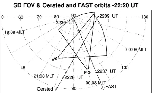
Fig. 1. Common field-of-view in mag-netic coordinates of the CUTLASS Hankasalmi (F) and Pikkvibær (E) radars at 22:20 UT, with the FAST and Ørsted trajectories superimposed.
three field-aligned currents. In the Northern Hemisphere for negativeBy, the convection consists of a velocity shear, with a westward plasma flow at the lower latitudes and an east-ward plasma flow at the higher latitudes. For positiveBy, the flow directions are reversed. The electron precipitation disappears close to the convection reversal boundary and is always located on the low-latitude side of the plasma flow.
Different techniques have been used to model the horizon-tal and parallel currents system (see Untiedt and Baumjo-hann, 1993, for a review). The “method of characteristics” (Amm, 1995, 1997, 1998) has allowed Kosch et al. (2000) to model a vortex associated with an auroral arc. The horizontal and field-aligned currents and the ionospheric conductivity distributions are deduced over a 200 km ×200 km region, based on ionospheric plasma velocities obtained with the STARE radar and magnetic field disturbances deduced from the Scandinavian Magnetometer Array (SMA). They showed that the plasma flow vortex was associated with an iono-spheric region of diverging horizontal electric field, equiva-lent to a downward field-aligned current, and corresponding to a region of decreased conductivities, as expected for an anticlockwise convection. This was the first observation of a black aurora from the ground.
In this paper, we present a case study on 12 January 2000 of a convection shear during relatively quiet and steady IMF conditions characterised by a positive Bz and a negative
By. This shear is representative of the negative By case of Taguchi et al. (1994). The data are obtained during a conjunction in the midnight sector between the Ørsted and FAST satellites, occurring over the common field of view of the CUTLASS pair of the SuperDARN radars. Ørsted crosses the common field of view of the radars between 22:10 and 22:16 UT and FAST 20 min later, between 22:30 and 22:36 UT, as shown on the schematic diagram of Fig. 1. The two satellite passes will be presented and modelled sep-arately since they are separated by 20 min. For the FAST
pass, field-aligned currents deduced from magnetic field per-turbations and ionospheric conductivities deduced from par-ticle precipitation will be used to determine the ionospheric convection profile along the orbit, by using the condition of current continuity. For the Ørsted pass, using the field-aligned currents deduced from Ørsted and ionospheric con-vection from SuperDARN radar data, the latitudinal profile of the ionospheric Pedersen conductance will be deduced, again from the condition of current continuity. A compari-son between the results obtained in both cases will be made, in order to feature the similarities and differences due to time and space separation. Auroral images from the Polar-UVI instrument will be used to emphasize the time evolution of the arc between the Ørsted and FAST satellite passes.
2 Instrumentation
The solar wind plasma and IMF data are provided by the ACE satellite, and images of the nightside auroral oval are from the Ultraviolet Imager (UVI) on board the Polar satel-lite.
The ionospheric convection velocities are given by the Hankasalmi (in Finland) and Pikkvibær (in Iceland) CUT-LASS radars. These radars belong to the SuperDARN chain of coherent HF radars, of which the main objective is to mon-itor the large-scale convection in the high-latitude ionosphere (Greenwald et al., 1995). Each radar measures the line-of-sight plasma flow velocity in the F-region of the ionosphere. The Hankasalmi and Pikkvibær radars share a common field of view, thus allowing one to obtain convection velocity vec-tors from the simultaneous measurement of two independent components. The SuperDARN radar beam is narrow, typ-ically 3.3◦ in azimuthal width. In the common mode, the
ACE IMF and solar wind data - 12/01/2000
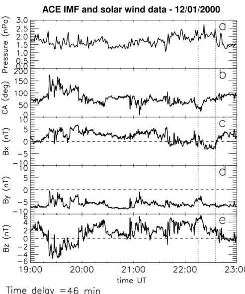
Fig. 2. Interplanetary magnetic field (IMF) and solar wind plasma data from the ACE spacecraft on 12 January 2000. Data are lagged by 46 min, to take into account the delay from the spacecraft to the ionosphere. (a)Solar wind pres-sure. (b)IMF clock angle. Panels(c),
(d)and(e)show ,respectively, the IMF Bx,ByandBzcomponents in GSM
co-ordinates.
In the present study, the radars were operated in a high reso-lution mode, in which a full scan was completed in 35 s.
During the first conjunction with the Ørsted satellite, field-aligned currents are deduced from magnetic field measure-ments. Ørsted is a Danish satellite, with a quasi-polar or-bit at about 600 km altitude. Its main objective is to per-form a precise mapping of the Earth’s magnetic field based on both a 3-axis and a scalar magnetometer. A detailed de-scription of the satellite and its instrumentation are given by Stauning et al. (2001). During the second conjunction with the FAST satellite, we will use field-aligned currents, elec-tric field and downgoing electron precipitation data. FAST is on a low-altitude, elliptical polar orbit and is designed to study small-scale structures of space plasma and acceleration mechanisms of particles (Carlson et al., 1998).
3 General context
Solar wind and IMF data from the ACE satellite are pre-sented in Fig. 2 (GSM coordinates). The propagation
de-lay between ACE and the dayside ionosphere is evaluated to about 46 min, by which the data in Fig. 2 have been lagged. The time of the Ørsted and FAST satellites’ passes over the radars’ field of view is indicated by the vertical dotted lines. The IMFBz remains positive for more than 2 h before the satellite passes. At the time of the satellites’ passes, the averageBz is +4 nT for Ørsted and +2 nT for FAST. The
Bycomponent remains negative and stable, with an average value of−6 nT, and theBxcomponent changes from positive to negative at the time of the Ørsted pass. Thus, a stable con-vection pattern is expected in the entire polar cap, character-istic of a strongly negativeByand a positiveBz. The average value of the IMF clock angle between 20:00 and 23:00 UT is 70◦. Taguchi and Hoffman (1996) have used a limiting value
of 70◦for the clock angle for the IMFBycontrol of the
con-vection, which suggests that it is presently the case. Freeman et al. (1993) (for strong total IMF (B =25 nT)) and Senior et al. (2002) (for smaller total IMF) have shown that a clock angle of 70◦represent the transition at which dayside
a
POLAR UVI - 12/01/2000 - 22:03:33 UT
Ørsted
b
POLAR UVI - 12/01/2000 - 22:14:35 UT
FAST
c
POLAR UVI - 12/01/2000 - 22:35:08 UT
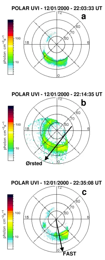
Fig. 3. Polar-UVI images in magnetic latitude-MLT coordinates.
(a)11 min before the Ørsted pass. (b) at the time of the Ørsted pass 22:14:35 UT, with the Ørsted trajectory superimposed. (c)at the time of the FAST pass 22:35:08 UT, with the FAST trajectory superimposed.
small clock angle (22:10–22:20 UT), no dayside reconnec-tion exists, but that the polar cap continues to evacuate on the nightside, fossil open flux created by dayside reconnection.
Between 19:00 and 23:00 UT, the mean solar wind dynamic pressure is 1.7 nPa, increasing to 2.2 nPa at the time of the satellites’ passes. The solar wind and IMF conditions cor-respond to a quiet and fairly steady magnetosphere, mainly controlled by the negativeBy, a situation similar to the sta-tistical studies of Taguchi (1992), Taguchi et al. (1994) and Taguchi and Hoffman (1996).
During the period of interest, Polar-UVI observations of the nightside auroral oval are available. The Polar-UVI im-ages obtained 11 min before the Ørsted pass (Fig. 3a), at the time of the Ørsted pass (Fig. 3b) and at the time of the FAST pass (Fig. 3c) illustrate the spatial structure and the tempo-ral variation of the nightside precipitation during the period and show that even if the magnetosphere is in a quiet con-figuration, the situation is, however, quite dynamic. Both satellite passes occur on the western edge of a precipitation zone covering the early morning sector. By comparing these 3 images, an apparent poleward motion of the auroral oval is observed in the midnight and early morning sector, espe-cially between the first 2 images, which corresponds to the time interval 22:05–22:15 UT when the clock angle is small-est (Fig. 2a). This shrinking of the polar cap size is in agree-ment with the hypothesis of a decrease in the open flux in the polar cap. The 3 images also illustrate intensity varia-tions of the precipitation pattern. The first and third images show a weak precipitation intensity while the second image shows an increase of the precipitation intensity. Moreover, examination of all the Polar images of the global time inter-val 22:00–23:00 UT indicates intensifications of the auroral precipitation about every 6 min, which confirms the dynam-ical situation. A maximum of precipitation is observed just before the Ørsted pass and a minimum of precipitation is ob-served during the FAST pass. Auroral quasi-periodic inten-sifications under similar IMF conditions have been already observed by de la Beaujardi`ere et al. (1994) and Senior et al. (2002).
4 Data presentation
4.1 Ionospheric convection
Figures 4a and b show the pattern of ionospheric convec-tion deduced from the CUTLASS radars, in the midnight sector for the two periods of interest: 22:10–22:16 UT, cor-responding to the Ørsted pass and 22:30–22:36 UT, corre-sponding to the FAST pass. The coordinates are Altitude-Adjusted Corrected GeoMagnetic (AACGM) (Baker and Wing, 1989) Magnetic Latitude (MLAT) and Magnetic Local Time (MLT). The maps have been averaged over 6 min in or-der to obtain more convection vectors. The projection along magnetic field lines of the Ørsted pass is superimposed on Fig. 4a and the projection of FAST pass on Fig. 4b.
60 75
90 105
120 135
60 65
70 75
80 85
90
1000m/s 12 January 2000
22:30:00 - 22:35:59 UT
60 75
90 105
120 135
60 65
70 75
80 85
90
1000m/s
SUPERDARN VELOCITY MAP
-
Thykkvibaer / Hankasalmi
12 January 2000 22:10:00 - 22:15:58 UT
FAST
Oersted
a
b
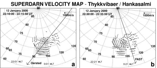
Fig. 4.Average (over 6 min) convection velocity maps of the CUTLASS radars in AACGM coordinates. (a)at the time of the Ørsted pass 22:10–22:16 UT, with the Ørsted trajectory superimposed. (b)at the time of the FAST pass 22:30–22:36 UT, with the FAST trajectory superimposed.
the lower latitudes. The dimensions of the structure are fairly large, with a 750 km extension in longitude and 400 km in latitude. The centre of the shear is at about 71.5◦MLAT. The
convection velocity is of the order of 600 m s−1on the edge of the structure. This semi-opened convection vortex encir-cles the early morning precipitation zone observed in Fig. 3b. The Ørsted trajectory superimposed on this map shows that Ørsted crosses the southwestern part of the convection vor-tex.
At the time of the FAST pass 20 min later, the convection (Fig. 4b) has changed significantly. A clockwise rotation of the vortical structure has occurred in the western part of the map. The velocities have the same amplitude, except for a small zone centred around 72◦MLAT and are composed of
larger and predominantly southward velocities. This south-ward flow indicates that the western part of the shear has evolved into an autonomous vortex, encircling the precipi-tation spot centred at 70◦MLAT and 00:00 MLT in Fig. 3c.
The trajectory superimposed on Fig. 4b shows that FAST crosses the eastern part of the convection pattern. In this region, almost the same directions of velocity are observed as at the time of the Ørsted pass. Around 75◦MLAT,
pre-dominantly eastward velocities are observed as well as west-ward velocities below 68.5◦MLAT. However, because data
points are missing in the SuperDARN convection map along the FAST orbit, the position of the velocity shear is not well defined. The north-south component of the DC electric field measured by FAST (Fig. 5a) and corresponding to the east-west component of the convection, indicates a convection reversal from eastward above 68.5◦MLAT to westward
be-low 68.5◦MLAT. Thus, the position of the convection shear
has evolved between the two satellites passes and is shifted southward at the time of the FAST pass. This observation confirms the evolution of the convection pattern. Unfortu-nately, the east-west component of the DC electric field at FAST, which could indicate a southward component of the
convection flow, is not available.
Differences between SuperDARN and FAST data can be explained by the spatial and temporal smoothing of the Su-perDARN convection maps. The electric field observed by FAST shows small-scale structures, in particular, a signif-icant reversal of the electric field gradient at 71◦MLAT,
where the electric field becomes almost zero. Notice also the strong positive electric field around 73◦MLAT, the amplitude
of which will be discussed later. These two features (gradient reversal at 71◦MLAT and peak electric field at 73◦MLAT)
are essential because, as we will show later, they are linked to field-aligned currents.
4.2 Field-aligned currents
The field-aligned currents associated with the convection shear are deduced from measurements made by the Ørsted satellite during the first period, and by the FAST satellite dur-ing the second period. The two satellites are movdur-ing equa-torward in the nightside. The magnetic perturbationδB is obtained by subtracting from the magnetic measurements the IGRF model of the internal magnetic field. The field-aligned currentsJkis deduced from Ampere’s law
Jk= 1 µo∇×
δB, (1)
assuming current sheets, the orientation of which is parallel toδB.
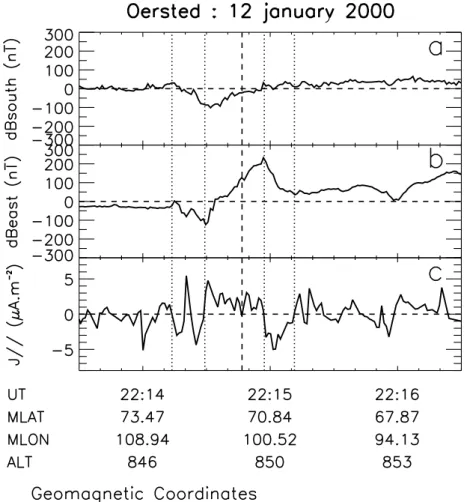
The magnetic perturbation at the Ørsted orbit and the asso-ciated field-aligned currents are shown in Fig. 6. The south-ward component (panel (a) is relatively weak, with varia-tions less than 100 nT and the eastward component (panel (b) has a sawtooth-like shape, with variations up to 250 nT. Large-scale variations reveal the existence of three current sheets. Between 22:13:00 and 22:14:30 UT (75.55◦ to
72.2◦MLAT), a smooth decrease in the eastward
Figure 5
Fig. 5. Electric and magnetic fields and field-aligned currents measured by FAST. (a) North-south component of the convection electric field. (b) and
(c)North-south and east-west compo-nents of the magnetic perturbations.
(d)Field-aligned currents intensity de-duced from the magnetic perturbations, averaged over 5 s. Dotted lines delin-eate the three parallel current sheets and the dashed line indicates the velocity shear.
low-latitudes which could be associated with a small-scale structure superimposed on the global structure. Then, be-tween 22:14:30 and 22:16:30 UT (72.2◦ to 66.3◦MLAT),
in spite of large perturbations, a general positive increase in this component is observed. Finally, at lower latitudes, be-tween 22:16:30 and 22:17:00 UT (66.3◦to 64.7◦MLAT), a
decrease in the perturbation (not shown in Fig. 6) is observed. These three perturbations agree with the statistical model of Iijima and Potemra (1976) around midnight which in-cludes three (downward-upward-downward) large-scale cur-rents, namely the morningside region-1, the eveningside regions-1 and -2 currents. The latitudinal extent of these currents is large, probably related to the positive IMFBz. Smaller scale perturbations with a larger amplitude are ob-served between 22:14:13 and 22:15:12 UT, at the inter-face between the morningside and the eveningside regions-1. Three intense current sheets deduced from these pertur-bations are represented in Fig. 6c, including from north to south: a downward current, an upward current centred on the
velocity shear and a downward current. These currents will be called, respectively, in the following sections:NH current for the High-latitude Negative (downward) current,P cur-rent for the Positive (upward) central curcur-rent andNLcurrent for the Low-latitude Negative current. These currents have quite large intensities, up to 5µA m−2 and their latitudinal width is, respectively, 65 km, 140 km and 75 km, forNH,P andNL. TheP current corresponds to the clockwise cir-culation of the convection semi-vortex, and theNH andNL currents correspond to the return currents of the convection-precipitation-upward current structure. The sign of these cur-rents agrees with the MTS current system of Taguchi (1992), for negativeBy.
Fig. 6. Magnetic field and field-aligned currents measured by Ørsted.
(a)North-south component. (b) East-west component.(c)Field-aligned cur-rents intensity averaged over 5 s. Dotted lines delineate the three parallel current sheets and the dashed line indicates the velocity shear.
Table 1.Angle between the directions of the magnetic East and of the 3 current sheets associated with the arc, along the Ørsted and FAST orbits. The angles are positive clockwise
Ørsted pass FAST pass
NHcurrent +68.0◦ −7.5◦
P current +39.5◦ −9.0◦ NLcurrent +15.5◦ −9.5◦
structure of the smaller scale parallel current is also simi-lar to the Ørsted case, with three current sheets embedded in region-1. These currents have the same sign for the two satellites passes. In the FAST case, the latitudinal width is, respectively, 125 km, 175 km and 160 km forNH,P andNL, which is slightly larger than the widths calculated along the Ørsted orbit. Table 1 shows the angle (positive anticlock-wise) between the magnetic isolatitude and the direction of the current sheet. The current sheets are nearly parallel to magnetic isolatitude lines at FAST, while they rotate along the Ørsted orbit. This important difference will be interpreted
in the Discussion section. The amplitude of theP andNL currents is smaller along the FAST orbit (Fig. 5d).
4.3 Particle precipitation
Figure 7a displays the electron precipitation measured by FAST. The precipitation pattern is highly structured with a strong precipitation above 71.3◦MLAT, from north to south,
a gap associated with theNLcurrent, and a weaker but more extended precipitation zone below 70◦MLAT. This
precipi-tation pattern is often observed in association with a convec-tion reversal, as, for instance, by Gurnett and Franck (1973). From the electron precipitation pattern, we determine the Pedersen and Hall conductances (height-integrated conduc-tivities), using Hardy’s model (Hardy et al., 1987):
6P =
40hEi 16+ hEi2
√
8 (2)
6H =0.45hEi5/86P, (3)
73.9°
70.5°
67.15°
63.7°
Mlat
0
4
8
12
0
50
100
150
<E>
Eflux
E
le
ct
ro
n
s
en
er
g
y
fl
u
x
(m
W
.m
-2)
a
n
d
a
v
er
a
g
e
en
er
g
y
(k
eV
)
C
o
n
d
u
ct
iv
it
ie
s
(S
)
Time after 2233:55 UT
b
c
0
4
8
12
16
20
0
50
100
150
P
H
a
E
n
er
g
y
(
eV
)_
P
A
=
0
°-3
3
°
1000
10000
L
o
g
(
eV
.c
m
-2_
s_
sr
_
eV
)
6.0
6.6
7.2
7.8
8.4
9.0
0
50
100
150
73.9°
70.5°
67.15°
63.7°
Mlat
0
4
8
12
0
50
100
150
<E>
Eflux
E
le
ct
ro
n
s
en
er
g
y
fl
u
x
(m
W
.m
-2)
a
n
d
a
v
er
a
g
e
en
er
g
y
(k
eV
)
C
o
n
d
u
ct
iv
it
ie
s
(S
)
Time after 2233:55 UT
b
c
0
4
8
12
16
20
0
50
100
150
P
H
73.9°
70.5°
67.15°
63.7°
Mlat
73.9°
70.5°
67.15°
63.7°
Mlat
0
4
8
12
0
50
100
150
<E>
Eflux
E
le
ct
ro
n
s
en
er
g
y
fl
u
x
(m
W
.m
-2)
a
n
d
a
v
er
a
g
e
en
er
g
y
(k
eV
)
C
o
n
d
u
ct
iv
it
ie
s
(S
)
Time after 2233:55 UT
b
c
0
4
8
12
16
20
0
50
100
150
P
H
a
E
n
er
g
y
(
eV
)_
P
A
=
0
°-3
3
°
1000
10000
L
o
g
(
eV
.c
m
-2_
s_
sr
_
eV
)
6.0
6.6
7.2
7.8
8.4
9.0
0
50
100
150
a
E
n
er
g
y
(
eV
)_
P
A
=
0
°-3
3
°
1000
10000
L
o
g
(
eV
.c
m
-2_
s_
sr
_
eV
)
6.0
6.6
7.2
7.8
8.4
9.0
0
50
100
150
6
6
FAST: 12 January 2000
Fig. 7. Electron precipitation mea-sured by FAST, between 22:33:55 and 22:36:25 UT.(a)Energy-flux diagram of the downgoing electrons, for the range 400 eV–30 keV. (b) Energy flux and average energy. (c)Pedersen and Hall ionospheric conductances. The po-sition of the three field-aligned current sheets deduced from FAST magnetic perturbations is superimposed (dotted lines).
keV with a low-energy cutoff at 500 eV, and8is the elec-trons energy flux in mW m−2(Fig. 7b). A basic ionospheric conductance is added to the Pedersen and Hall conductances, in order to take into account the faint solar ionisation. For the zenith angle and the MLT prevailing during the observations, a value of 1.5 S is chosen (Senior, 1991). The resulting con-ductance profiles are shown in Fig. 7c. The concon-ductances are large in the electron precipitation regions, reaching up to 15 S. The Hall and Pedersen conductance profiles are simi-lar. Strong gradients occur on the edges of the high-latitude precipitation region.
5 Simulation
Based on this detailed data set, including convection veloci-ties, conductances and parallel currents, models can be built,
based on the current continuity equation:
Jk= −6P(∇⊥·E⊥)−E⊥·∇⊥6P+(b×E⊥)·∇⊥6H,(4) where b is the unit vector parallel to the Earth’s magnetic field. In this expression, the first term on the right-hand side represents the contribution to the parallel current density of the ionospheric electric field gradients, which can be deduced from the convection velocity. The second and third terms represent the contribution of the conductance gradients de-duced from particle precipitation. Because satellite measure-ments are made only along the orbit, they do not provide sufficient inputs for a full two-dimensional model (2-D). 5.1 One-dimensional model
Fig. 8. Inputs (a and b) and result (c) parameters of the 1-D simulation along the FAST orbit.(a)Ionospheric Peder-sen conductance.(b)Field-aligned cur-rent measured by FAST.(c)Modelled (solid) and experimental (dotted line) east-west convection velocity. Dotted lines delineate the three parallel current sheets and the dashed line indicates the velocity shear.
wherex andy represent the eastward and northward direc-tions, and assuming a vertical magnetic field, relation (4) be-comes:
dVx(y)
dy +
1 6P(y)
d6P(y)
dy Vx(y)
= B6Jk
P(y)+ 1 6P(y)
d6H(y)
dy Vy(y). (5)
A usual simplification is to assume a constant Hall-to-Pedersen ratio of 1, well supported by the conductance pro-files along the FAST orbit (Fig. 7c)
dVx(y)
dy +
1 6P(y)
d6P(y)
dy
Vx(y)−Vy(y)=
J⊥ B6P(y)
.(6) This equation can be regarded either as an algebraic equation giving the parallel current density or as a differential equa-tion which governs the latitudinal profile of either the longi-tudinal component of the convection velocity or the Peder-sen conductance, depending upon the parameters which are measured. In the latter cases, additional information on the Vycomponent is necessary. We use relation (6) successively along the FAST and Ørsted orbits, in order to model the un-known (or less precisely measured) parameters.
5.1.1 Simulation along the FAST orbit
Along the FAST orbit, field-aligned currents have been mea-sured and ionospheric conductances have been deduced from particle precipitation. On the other hand, as mentioned ear-lier, the east-west component of the DC electric field (giv-ing the north-south component of the convection velocity) is not available on board the FAST satellite. Although Su-perDARN convection vectors are very scarce in the region of the FAST trajectory, vectors at the east of the orbit, be-tween 65◦and 75◦MLAT (Fig. 4b), are along the magnetic
isolatitude lines. Consequently, we have chosenVy(y)=0. Using field-aligned currents and conductances as inputs, re-lation (6) is integrated on the full latitudinal interval from 64◦
to 74◦MLAT, with the fourth-order Runge-Kutta algorithm,
in order to deduce the longitudinal component of the convec-tion velocity. An initial value of the longitudinal component of the convection of 600 m s−1is used at 74◦MLAT, in
ei-Fig. 9. Inputs (a and b) and result (c) parameters of the 1-D simulation along the Ørsted orbit. (a) East-west con-vection profile deduced from the Su-perDARN convection map. (b) Field-aligned current measured by Ørsted.
(c)Modelled ionospheric Pedersen con-ductance. Dotted lines delineate the three parallel current sheets and the dashed line indicates the velocity shear.
ther with the east-west component of the convection velocity deduced from the north-south component of the electric field measured by FAST (dash-dotted line in Fig. 8) or with the SuperDARN measurements. Between 64◦ and 74◦MLAT,
the modelled and experimental data are very similar in posi-tion and amplitude, except for the discrepancy in amplitude observed above 72.5◦MLAT. The large velocity peak centred
at 72.9◦MLAT is observed both in modelled and
experimen-tal data, but the amplitudes are very different. The reason for the difference between experimental and modelled amplitude of the electric peak will be explained in the Discussion sec-tion.
5.1.2 Simulation along the Ørsted orbit
Along the Ørsted orbit, field-aligned currents, convection velocity (and consequently convection electric field) are known. Using these inputs, relation (6) can be integrated, in order to deduce the Pedersen conductance. The inputs and the resulting latitudinal component of the Pedersen conduc-tance along the Ørsted orbit are presented in Fig. 9. In a pre-liminary step, the experimental convection map (Fig. 4a) has been fitted to an analytic model. In this model, the east-west component of the ionospheric convection velocity Vx(y)
along the Ørsted orbit is characterised by a velocity shear at 71.5◦MLAT (Fig. 9a), and the north-south component of
the convection velocity is taken atVy(y)= −Vx(y)/2 above the velocity shear andVy(y) = 0 below. As a test of the role played by the north-south component of the velocity, we have also integrated Eq. (6) with a purely longitudinal veloc-ity (Vy(y)=0 everywhere). The result shows no significant difference in the conductance profile. At the velocity shear, relation (6) simplifies and the Pedersen conductance is ob-tained directly from the parallel current and the velocity gra-dient, which provides an initial value for integration from this point, independently on both sides of the convection rever-sal. The conductance at the velocity shear is 6S, a realistic value, since the discontinuity is situated on the low-latitude side of both theP current and the electron precipitation and thus, corresponds to the lower side of the conductance gradi-ent. We have chosen not to model the Pedersen conductivity in the region of theNL current, in order to avoid negative values. The integration starts again at 70.3◦MLAT, beyond
AACGM Longitude in degrees
96 98 100 102 104 106 108
12 S
AA CGM Latitude in degrees
70 70.5
71 72 71.5 73 72.5
73.5
AA CGM Latitude in degrees
70 70.5 71 71.5 72 72.5
73 73.5
AACGM Longitude in degrees
96 98 100 102 104 106 108
+ / - 3 µA/m²
Oersted Oersted
Figure 10
(a)
(b)
Oersted: 12 January 2000
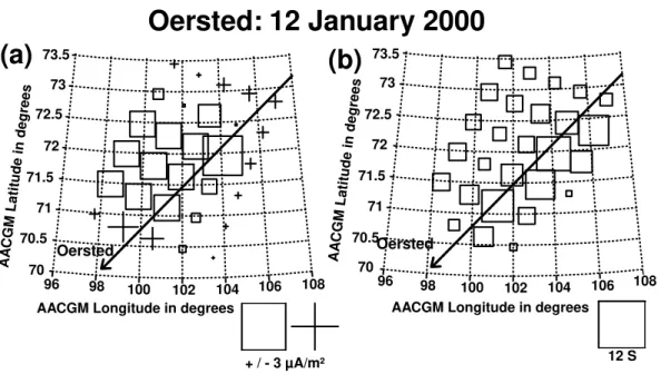
Fig. 10.Two-dimensional distributions in AACGM coordinates(a)of the field-aligned current deduced from the Ørsted measurements and
(b)of the modelled Pedersen conductance, assuming a Hall-to-Pedersen conductance ratio equal to 1. The parameters are plotted in the form of symbols, of which the size is proportional to the intensity of the parameter. Squares and crosses represent, respectively, the upward currents and downward currents. The projection of the Ørsted orbit is also shown.
7 S, probably associated with the eveningside region-2 of a large-scale currents. The fact that we could not model the conductance in the region of theNL current shows that the 1-D model is not well adapted for the Ørsted orbit. However, in the regions where the conductance can be modelled, simi-larities between the experimental profile of Pedersen conduc-tance along the FAST orbit and the modelled conducconduc-tance along the Ørsted orbit are observed, although the time and longitude of FAST and Ørsted are different. Both poleward and equatorward of the shear, the number and the relative amplitude of the peaks are the same. A small global latitu-dinal shift, of the order of 0.2◦between the two profiles, is
observed.
5.2 Two-dimensional model along the Ørsted orbit Since along the Ørsted orbit the 1-D model is not successful in providing a full latitudinal profile of the Pedersen conduc-tance, we have tested a 2-D model also based on the current continuity equation, obtained from the “FAC-based method of characteristics” developed by Amm (2002). This method allows one to calculate the distribution of ionospheric con-ductances and actual currents from the two-dimensional pro-files of ionospheric electric field and of field-aligned currents mapped to the ionosphere, with the Hall-to-Pedersen conduc-tance ratioαbeing given. Theαratio is taken to be 1 (a re-alistic value for low magnetic activity; see also the ratio of FAST conductances modelled in Fig. 7). The electric field pattern responsible of the convection vortex is given by the SuperDARN radars. Note that the centre of the convection vortex is located at 72.3◦MLAT and 101.3◦Magnetic
Longi-tude (MLON), at a slightly higher latiLongi-tude than the shear
ob-served along the Ørsted orbit. However, because Ørsted pro-vides FAC only along its orbit, it is necessary to extrapolate Ørsted data to a 2-D FAC distribution. The field-aligned cur-rent at each grid point is given by the mean of the FAC at the points of the Ørsted orbit situated at the same distance from the centre of the FAC. In order to have continuity of the cur-rent, the mean is weighted by the inverse distance between the data point and the Ørsted point. Before this process, the Ørsted data have been averaged to a scale of∼50 km, cor-responding to the spatial resolution of SuperDARN. For the grid points at a radial distance smaller than the distance be-tween the Ørsted orbit and the centre of the FAC distribution, the attributed value of FAC is equal to+1.65µA m−2. This value corresponds to the 50 km average of the closest portion of the Ørsted path from the vortex centre. The distribution of the FAC is plotted in AACGM coordinates in Fig. 10a. The FAC configuration shows a circular central positive cur-rent (theP current) surrounded on its northward, southward and eastward sides by a downward current (corresponding to theNL andNH currents) with a smaller amplitude around
maximum in its larger dimension. At the centre of the mod-elled positive current, the conductance decreases to about 3 S. This surprising result will be explained in the next sec-tion.
6 Discussion
6.1 FAST results and the validity of the one-dimensional model
A strong similarity is observed between the experimental and the 1-D modelled profiles of the east-west convection (Fig. 8c). The forms of the peak around 72.9◦MLAT, the
gradient reversal at 71◦MLAT and the convection shear at
68.5 MLAT are well reproduced by the simulation with only a small latitudinal shift of the convection shear. The ampli-tudes are also similar, except for the peak at 72.9◦MLAT,
where the experimental peak is three times larger than mod-elled. Clearly, the amplitude is not realistic, suggesting a non-standard behaviour of the electric antenna in theNH re-gion.
The NH current of the triple parallel currents’ structure (Fig. 8b) is very intense, and its maximum is associated with a strong electric field gradient. This result confirms earlier studies, in which intense electric fields are observed in the downward FAC region adjacent to a brightening arc (Opgenoorth et al., 1990; Aikio et al., 1993, 2002). However, in our case, the latitudinal extent of the global arc, of theNH downward FAC, and of the associated electric field, are con-siderably larger. Moreover, a strong conductance gradient at the polar side of the precipitation and opposite to the electric field gradient occurs just at the boundary between theNH and theP currents. TheP parallel current is associated with the conductance gradients related to the equatorward side of the electron precipitation. In theP current, the electric field gradient is weak. At the boundary between theP and the NLcurrents, the electric field gradient reverses, but not the sign of the electric field. TheNLcurrent is associated with the electric field gradient alone, since the conductance is al-most constant in this region. As shown by relation (6), the electric field gradient is proportional to the parallel current, under these circumstances. It is fairly large in the 0.5◦
latitu-dinal range where the parallel current is large (1.5µA m−2). In conclusion, the arc has a large longitudinal extent and presents a central positive current with negative parallel cur-rents on both sides. Electric field gradients drive the negative currents, while, on the opposite, the conductance gradient on the equatorward side of the main precipitation drives theP current.
The similarity between modelled and experimental pro-files of the east-west convection velocity along the FAST orbit also supports the latitudinal one-dimensional hypoth-esis. The FAST trajectory is rather in the latitudinal part of the convection pattern, at the east of the vortex. These re-sults are confirmed by the fact that the direction of the three current sheets detected by FAST are almost parallel to the
magnetic east-west direction (Table 1). The 1-D model is very efficient in the case of a purely latitudinal convection pattern, as shown by the results obtained along the FAST or-bit. Figure 11 shows the instantaneous radial velocity maps of the two CUTLASS radars, at the time of the FAST pass. These maps will be used for comparing the experimental and modelled east-west convection profiles. Although the Pikkvibær map contains large data gaps, several patches of eastward velocities above 69◦MLAT (red and orange
veloc-ities) and several patches of westward velocities (blue) be-low 69◦MLAT are observed. This convection reversal agrees
well with the convection shear observed around 68.5◦MLAT
by FAST. The Hankasalmi map is more detailed, but the ve-locity component measured with this radar is predominantly in the north-south direction. As the convection velocities are mainly east-west, the Hankasalmi map does not provide the most significant component of the convection. However, several features of this map confirm the results of the mod-elling. Exactly on the FAST trajectory, an enhancement of the eastward convection is observed (a small east-west band of orange and yellow velocities), exactly at the latitude of the strong peak of eastward velocities measured by FAST, at 73◦MLAT. Assuming a purely longitudinal flow, this
line-of-sight velocity turns into a flow velocity of∼2000 m s−1, a value which agrees quantitatively with the modelled result of 1700 m s−1 (Fig. 8). Further south, FAST crosses a re-gion of predominantly eastward but smaller velocities and is tangent to a complex structure of the radial velocities corre-sponding to a strong decrease in the velocity and associated with the gradient reversal measured by FAST, at 71◦MLAT.
Then, at about 69◦MLAT, a real east-west convection shear
is observed associated with the convection reversal also ob-served on the Pikkvibær map and on the FAST east-west convection profiles. These similarities between FAST and SuperDARN confirm the validity of the modelled east-west convection profile obtained with the 1-D model.
6.2 Ørsted results
cur-60
80
100 120
140 60
65 70
75 80
85 90
-800 -600 -400 -200 0 200 400 600 800
m/s
THIKKVIBAER: vel 12 January 20002233 37s
10.335 MHz 60
80
100 120
140 60
65 70
75 80
85 90
-800 -600 -400 -200 0 200 400 600 800
m/s
SUPERDARN PARAMETER MAP
HANKASALMI: vel 12 January 20002233 27s
9.950 MHz
FAST
FAST
a
b
Fig. 11. Line-of-sight velocity maps of the Pikkvibær (top panel) and Hankasalmi (bottom panel) radars in AACGM coordinates, at the time of the FAST pass, with the FAST orbit super-imposed.
rent of the vortex. This is why we have used a 2-D model to obtain more realistic results of the conductance profile along the Ørsted orbit.
However, the FAC input to the 2-D model is known only along the Ørsted orbit and has to be extrapolated elsewhere. In particular, the density of the central part of theP current is chosen to be constant, which is probably not the case. This incorrect description of the centre of theP current can ex-plain the unexpected small values of conductance located in the vicinity of the vortex centre. For these reasons, the con-ductance profile deduced from this 2-D model is expected to be more accurate close to the Ørsted trajectory than far from it, because the FAC evaluation is also less acurate with in-creasing distance from the Ørsted orbit. Thus, the 2-D mod-elling also presents insufficiencies but allows for a correct description of the conductance along the Ørsted orbit.
If we compare the results of the conductance profile ob-tained with the 1-D and the 2-D models along the Ørsted or-bit, we note several differences. The highest conductance
ob-tained with the 2-D model (8 S) is slightly smaller than with the 1-D model (10.5 S), which can be explained by the spa-tial smoothing involved. Moreover, with the 2-D model, the spatial extent of the maximum of conductance is large and coincides with theP current, contrary to the 1-D model, for which the maximum of conductance is narrow and located at the boundary between theP andNH currents, with theP current being associated with a conductance gradient. This last result seems to better support the 2-D model, because it is more likely that in an arc maintained by FACs, the down-ward electron precipitation associated with the conductance increase is coupled with the centre of the upward current and that the conductance gradients are located at the boundaries of the upward current (Burch et al., 1976; Opgenoorth et al., 1990). In spite of the above differences, both models give es-sentially the same global elongated shape of the precipitation pattern.
Ørsted
22:15 UT
22:35 UT
a
b
FAST
Fig. 12.Schematic representations of the ionospheric precipitation (grey surface) and convection pattern (solid lines) with the convec-tion velocity shear superimposed (dotted line). (a)At the time of the Ørsted pass with the Ørsted trajectory superimposed (dashed line). (b)At the time of the FAST pass, with the FAST trajectory superimposed (dashed line).
and the need to model the 2-D parallel current pattern from 1-D satellite measurements in the 2-D case. Although the validity of these hypotheses cannot be checked from the ex-perimental data set, they are probably not fully justified, as shown by the insufficiencies of the results. However, these two models are the best which can be constructed from this data set. The results of both models show similarities con-firming the general structure of the precipitation pattern dur-ing the Ørsted pass (described precisely in the next subsec-tion).
6.3 Time evolution
This double conjunction can be used to understand the time evolution of the current and precipitation patterns between the Ørsted and FAST passes. First, a global northward motion of the structure is observed between the two satel-lites passes. Thus, the triple current-sheets system has been shifted northward by about 1◦MLAT during the 20 min-time
interval. The precipitation region associated with theP cur-rent is also shifted northward. Moreover, strong modifi-cations of the convection-precipitation pattern are also ob-served between the two satellites passes. In both cases, the Polar images show a continuous band of precipitation in the
early morning sector, extending eastward to the limit of the field of view at about 03:00 MLT. Both satellites’ passes oc-cur on the western edge of this precipitation where the pat-tern modifications occur. Figure 12a and b show schematic representations of the convection-precipitation pattern at the times of the Ørsted and FAST passes, deduced from the SuperDARN convection maps (Fig. 4a, b) and from the Polar-UVI images (Fig. 3b, c). During the Ørsted pass (Fig. 12a), the main region of precipitation (grey surface) has a quasi-continuous east-west extent limited westward of around 23:30 MLT and is associated with the semi-elliptical clockwise vortex (solid lines) also having mainly a large east-west extent and closed on the east-western side. However, a clockwise rotation of the vortex is observed with respect to the main region of precipitation located at the east and also a slight narrowing of the precipitation region just eastward of the Ørsted pass (dashed line). Thus, Ørsted crosses the vortical part of the precipitation-convection pattern which is probably more two-dimensional than the region situated at later MLTs. This justifies the conclusion made in the previ-ous section, that the 1-D model is not adapted to the Ørsted case. At the time of the FAST pass (Fig. 12b), the western part of the precipitation (grey surface) has separated from the main precipitation to form a single isolated spot associated with the circular convection vortex at the west (solid lines). An intensification of southward velocities is then observed to close the eastern side of the vortex and keep it isolated, supporting the idea, that this part of the convection pattern is now fully two-dimensional compared to the eastward part of the precipitation which keeps the purely latitudinal struc-ture. Thus, this eastward precipitation forms a double purely latitudinal structure with a gap at the centre where the NL current is observed, supported by the purely east-west con-vection lines in this region. FAST crosses this second part of the precipitation, which explains why the one-dimensional model is valid along its trajectory.
Finally, we can also note a strong 3◦MLAT southward
shift of the convection velocity shear between the two satel-lites passes (dotted line of Fig. 12a and b). Thus, at the time of the FAST pass, the arc is no longer associated with the east-west convection shear as observed along the Ørsted orbit and generally in previous studies (Gurnett and Frank, 1973; Burch et al., 1976; Taguchi, 1992; Taguchi et al., 1994), but simply with a reversal of the gradient in the east-west con-vection velocity. These observations imply that the system of 3 field-aligned current sheets is not necessarily associated with a convection shear, in order to maintain the divergence of the Pedersen currents.
different between Ørsted and FAST.
Is the current system balanced? We have checked the bal-ance of the 3 current-sheets system. Based on the 1-D lati-tudinal profile of the current structure along the FAST orbit, we have integrated the total positive and negative latitudinal currents. The total positive current is 0.294 A m−1and the sum of the two negative currents is−0.309 A m−1, showing that positive and negative currents are almost equal. Thus we can conclude that the 3 current-sheets system is balanced and isolated from the rest of the auroral oval. Along the Ørsted orbit, the 3 current-sheets system is not one-dimensional and consequently, the balance between negative and positive cur-rents cannot be verified.
6.4 Magnetospheric coupling
The simultaneous appearance of high energy population (up to 1 keV) in the ion flux and of the inverted-V structures in the downgoing electrons’ diagram associated with theP cur-rent of the 3 curcur-rent sheets suggests that this structure is localised on the boundary between opened and closed field lines, but is, however, essentially on closed field lines. This structure has its magnetospheric origin in the magnetotail, probably in the Plasma Sheet Boundary Layer (PSBL), since the ions’ and electrons’ high mean energies and the inverted-V structures of the electron precipitation are typical of this magnetospheric region (Eastman et al., 1984; Huang et al., 1984).
Another feature related to the magnetospheric origin of the particles reveals the dynamical situation of the nightside ionosphere, already noted in the General Context section. Between about 22:00 and 00:00 UT, intensifications of the electron precipitation are observed every 6 min in the whole nightside ionosphere. Ørsted and FAST cross the auroral oval just before a maximum and during a minimum of the precipitation, respectively. This probably explains the larger values of the parallel currents during the Ørsted pass than during the FAST pass. The periodic intensifications of the precipitation pattern are probably due to regular injections of particles associated with reconnection in the magnetotail.
7 Summary
Two successive conjunctions between the CUTLASS Super-DARN radars and the Ørsted and FAST satellites occur in the nightside ionosphere on 12 January 2000, between 22:10 and 22:40 UT, and around 00:00 MLT. The Polar-UVI satel-lite and the IMAGE magnetometer data are also available in this region, at the same period. The large data set obtained during these conjunctions allows one to understand the struc-ture and the time evolution of a nightside arc associated with a convection shear, during relatively quiet interplanetary con-ditions (stable IMFBz>0 andBy <0 and stable solar wind pressure). Three field-aligned currents, one upward and two downward on each side, in order to close the global current system, are observed by the two satellites.
Modelling of the arc along the two satellites passes, based on the current continuity equation, allows one to understand the association between the electric field and conductance gradients which are the source of parallel currents. More-over, the 20-min time lag between the two satellites’ passes and the time series of SuperDARN maps and Polar images, allow one to describe the evolution of the nightside arc. Peri-odic enhancements of the convection and electron precipita-tion associated with the arc are observed, probably associated with regular, periodic injections of particles due to reconnec-tion in the magnetotail. A general northward moreconnec-tion of the electron precipitation and field-aligned currents is observed between the two satellites’ passes. In addition, a reorgani-zation of the precipitation and of the convection patterns in the vicinity of the arc occur, characterised by a dissociation of the electron precipitation into a single spot at the western edge of the arc, whereas the convection shear at the eastern side is shifted by 3◦MLAT southward implying that the arc
and the associated system of 3 field-aligned current sheets are no longer associated with the convection shear, in order to maintain the divergence of the Pedersen currents.
Acknowledgements. The authors acknowledge M. Berthomier for helpful discussions concerning the FAST data interpretation. The CUTLASS HF radars are deployed and operated by the Uni-versity of Leicester, and are jointly funded by the UK Par-ticle Physics and Astronomy Research Council (grant number PPA/R/R/1997/00256), the Finnish Meteorological Institute, and the Swedish Institute of Space Physics. The Ørsted satellite project is funded by the Danish Ministry of Research and Information Tech-nology, the Ministry of Trade and Industry, and the Danish Research Councils. The Ørsted satellite is operated by TERMA Electronics and the Danish Meteorological Institute (DMI). FAST data analysis at the University of California in Berkeley was supported through NASA grant NAG5-3596. The authors acknowledge the principal investigator N. Ness and the ACE Science Center for providing the ACE magnetic field data and the Finnish Meteorological Institute for providing the IMAGE data.
The Editor in Chief thanks A. D. M. Walker and A. Aikio for their help in evaluating this paper.
References
Aikio, A. T., Lakkala, T., Kozlovsky, A., and Williams, P. J. S.: Electric fields and currents of stable drifting auro-ral arcs in the evening sectors, J. Geophys. Res., 107, 1424, doi:10.1029/2001JA009172, 2002.
Aikio, A. T., Marklund, G. T., Woch, J., and Potemra, T. A.: Small-scale structures in the high-latitude auroral electric field, Ann. Geophysicae, 13, 84–94, 1995.
Aikio, A. T., Opgenoorth, H. J., Persson, M. A. L., and Kaila, K. U.: Ground-based measurements of an arc-associated electric field, J. Atmos. Terr. Phys., 55, 797–808, 1993.
Amm, O.: Ionospheric elementary current systems in spherical co-ordinates and their application, J. Geomag. Geoelectr., 49, 947, 1997.
Amm, O.: Method of characteristics for calculating ionospheric electrodynamics from multisatellite and ground-based radar data, J. Geophys. Res., 107, 1270, 2002.
Amm, O.: Method of characteristics in spherical geometry applied to a Harang Discontinuity situation, Ann. Geophysicae, 16, 413– 424, 1998.
Baker, K. B. and Wing, S.: A new magnetic coordinate system for conjugate studies at high latitudes, J. Geophys. Res., 94, 9139– 9143, 1989.
Burch, J. L., Lennartsson, W., Hanson, W. B., Heelis, R. A., Hoff-man, J. H., and HoffHoff-man, R. A.: Properties of spikelike shear flow reversal observed in the auroral plasma by Atmosphere Ex-plorer C, J. Geophys. Res., 81, 3886–3896, 1976.
Carlson, C. W., Pfaff, R. F., and Watzin, J. G.: The Fast Auroral SnapshoT (FAST) mission, Geophys. Res. Lett., 25, 2013–2016, 1998.
De la Beaujardi`ere, O., Lyons, R., Ruohoniemi, J. M., Friis-Christensen, E., Danielsen, C., Rich, F. J., and Newell, P. T.: Quiet-time intensifications along the poleward auroral boundary near midnight, J. Geophys. Res., 99, 287–298, 1994.
De la Beaujardi`ere, O., Vondrak, R., and Baron, M.: Radar observa-tions of electric fields and currents associated with auroral arcs, J. Geophys. Res., 82, 5051–5062, 1977.
Eastman, T. E., Franck, L. A., Peterson, W. K., and Lennartsson, W.: The Plasma Sheet Boundary Layer, J. Geophys. Res., 89, 1553–1572, 1984.
Freeman, M. P, Farrugia, C. J., Burlaga, L. F., Hairston, M. R., Greenspan, M. E., Ruohoniemi, J. M., and Lepping, R. P.: The interaction of a magnetic cloud with the Earth: Ionospheric con-vection in the northern and southern hemispheres for a wide range of quasi-steady interplanetary magnetic field convection, J. Geophys. Res., 98, 7633–7655, 1993.
Greenwald, R. A., Baker, K. B., Dudeney, J. R., Pinnock, M., Jones, T. B., Thomas, E. C., Villain, J.-P., Cerisier, J.-C., Senior, C., Hanuise, C., Hunsucker, R. D., Sofko, G., Koehler, J., Nielsen, E., Pellinen, R., Walker, A. D. M., Sato, N., and Yamagishi, H.: DARN/SuperDARN: A global view of high-latitude convection, Space Sci. Rev., 71, 761–796, 1995.
Gurnett, D. A. and Franck, L. A.: Observed Relationships between electric fields and auroral particle precipitation, J. Geophys. Res., 78, 145–170, 1973.
Hardy, D. A., Gussenhoven, M. S., Raistrick, R., and McNeil, W. J.: Statistical and Functional Representations of the Pattern of auro-ral energy flux, number flux, and conductivity, J. Geophys. Res., 92, 12 275–12 294, 1987.
Huang, C. Y., Frank, L. A., and Eastman, T. E.: High-altitude ob-servations of an intense inverted V event, J. Geophys. Res., 89, 7423–7430, 1984.
Iijima, T. and Potemra, T. A.: Field-aligned currents in the dayside cusp observed by Triad, J. Geophys. Res., 81, 5971–5979, 1976. Janhunen, P., Olsson, A., Amm, O., and Kauristie, K.: Characteris-tics of a stable arc based on FAST and MIRACLE observations, Ann. Geophysicae, 18, 152–160, 2000.
Johnson, M. L., Murphree, J. S., Marklund, G. T., and Karlsson, T.: Progress on relating forms and electric field patterns, J. Geophys. Res., 103, 4271–4284, 1998.
Kosch, M. J., Amm, O., and Scourfield, M. W. J.: A plasma vortex revisited: The importance of including ionospheric conductivity measurements, J. Geophys. Res., 105, 24 889–24 898, 2000. Marklund, G.: Auroral Arc classification scheme based on the
ob-served arc-associated electric field pattern, Planet. Space Sci., 32, 193–211, 1984.
Marklund, G., Sandahl, I., and Opgenoorth, H. J.: A study of the dynamics of a discrete auroral arc, Planet. Space Sci., 30, 179– 197, 1982.
Marklund, G., Baumjohann, W., and Sandahl, I.: Rocket and ground-based study of an auroral breakup event, Planet. Space Sci., 31, 207–220, 1983.
Opgenoorth, H. J., Haggstrom, I., Williams, P. J. S., and Jones, G. O. L.: Regions of strongly enhanced perpendicular electric fields adjacent to aurorals arcs, J. Atmos. Terr. Phys., 52, 449– 458, 1990.
Senior, C., Cerisier, J.-C., Rich, F. J., Lester, M., and Parks, G. K.: Strong sunward propagating, flow bursts in the night sector dur-ing quiet solar wind conditions: SuperDARN and satellite obser-vations, Ann. Geophysicae, 20, 771–779, 2002.
Senior, C.: Solar and particle contributions to auroral height-integrated conductivities from EISCAT data: A statistical study, Ann. Geophysicae, 9, 449–460, 1991.
Stauning, P., Primdahl, F., Watermann, J., and Rasmussen, O.: IMF By-related Cusp currents observed from the Ørsted satellite and
from ground, Geophys. Res. Lett., 28, 99–102, 2001.
Taguchi, S. and Hoffman, R. A.: Ionospheric plasma convection in the midnight sector for northward interplanetary magnetic field, J. Geomag. Geoelectr., 48, 925–933, 1996.
Taguchi, S.:By-controlled field-aligned currents near midnight
au-roral oval during northward Interplanetary magnetic field, J. Geo-phys. Res., 97, 12 231–12 243, 1992.
Taguchi, S., Sugiura, M., Iyemori, T., Winningham, J. D., and Slavin, J. A.:By-controlled convection and field-aligned currents
near midnight auroral oval for northward interplanetary magnetic field, J. Geophys. Res., 99, 6027–6044, 1994.
Untiedt, J. and Baumjohann, W.: Studies of polar current systems, Space Sci. Rev., 63, 245–390, 1993.