Performance of Exchange Rate Forecast
Using Distance-Based
Fuzzy Time Series
Lazim Abdullah Department of Mathematics Faculty of Science and Technology
University Malaysia Terengganu Malaysia
Abstract—Fuzzy time series model has been employed by many researchers in forecasting activities such as students’ enrolment, temperature fluctuations and stock prices. The existing fuzzy time series models require exact match of the fuzzy logic relationships to calculate the forecasted value. However, in real life applications, the exact match of fuzzy logic relationships is not possible. Thus, an improved fuzzy time series model termed as distance-based fuzzy time series model was proposed to remedy this shortcoming and successfully tested to the case of exchange rate data of New Taiwan Dollar (NTD) against United States Dollar (USD). The model was reportedly outperformed the artificial neural network and random walk models for the NTD against USD exchange rate. However, the performance of exchange rate using the distance-based fuzzy times series model for other currencies is still not fully explored. This paper forecasts the exchange rate of Malaysian Ringgit (MYR) against USD and tests the performance of the exchange rate using a distance-based fuzzy time series model. Data of the exchange rate USD against MYR from 11 August 2009 to 15 September 2009 were tested to the forecasting model. A sample of performance comparison between data sets of MYR against USD and NTD against USD was conducted. Under the same forecasting model, it is found that the forecasting errors for MYR against USD were smaller than NTD against USD exchange rate. The experiment results show that the forecasted exchange rate of MYR against USD has performed better under the distance-based fuzzy time series model.
Keyword- Fuzzy time series, Exchange rate, Euclidean distance, Fuzzy rules, Forecasting error
I. INTRODUCTION
Foreign exchange market plays an important role as the mechanism for providing access to foreign currencies so that transactions can be made across borders. Foreign exchange simply means the process of buying one currency and selling of another simultaneously. In other words, the currency of one country is exchanged for those of another. The foreign exchange market is the market in which buying and selling of different currencies take place. The price of one currency in terms of another is called an exchange rate. Among the important behaviours of exchange rate are fluctuation, volatility, uncertainty and unpredictable. It is very much similar with the nature of stock market thus open for forecasting activities. Research in forecasting of stock market has been heavily paid attention by many scholars research. Forecasting in exchange rate is somehow given less attention. Perhaps it was due to the perception that exchange rate is less important in daily economic transactions. However with the advent of intelligent knowledge, various methods in forecasting have been proposed and tested to exchange rate. Chen and Leung [1], for example, proposed Bayesian Vector Error Correction Model to forecast currency exchange rates for three major Asia Pacific economies – Korea, Japan, and Australia. In 2007, Panda and Narasimhan [2] predicted the exchange rate of Indian Rupee and US dollar by artificial neural networks. Furthermore, Anastasakis and Mort [3] apply both parametric (neural networks with active neurons) and nonparametric (analog complexing) self-organizing modelling method for the daily prediction of the exchange rate market. Every proposed method has shown some strengths and advantages but there was hardly seen one single method that can fit for all forecasting environment. For example, in regressive methods, number of data is one of the important assumptions that need to be fulfilled. As to overcome some these limitations, Song and Chissom [4], [5] introduced fuzzy time series. Song and Chissom applied the fuzzy theory in time series and provided the definitions and framework of fuzzy time series. The most usefulness of the fuzzy time series approach is its ability to deal with a very small set of data and the linearity assumption need not to be considered.
outlined its modelling by means of fuzzy relational equations and approximate reasoning. Since then, many researchers used the model proposed by Song and Chissom to solve various forecasting problems such as university enrolment [7], [8], [9] direct tax collection [10], stock index [11], [12], [13] and temperature [14]. Many past researchers were trying hard to improve the existing fuzzy time series model in order to get a better prediction. Lee et al.[15], for example, proposed to allow more than one factor in a fuzzy time series. Chen et al. [16] proposed a new fuzzy time series method which incorporated the concept of Fibonacci sequence for stock price forecasting. Leu et al. [17] proposed distance-based fuzzy time series and tested to the exchange rate data released by the Central Bank of Taiwan. Distance-based fuzzy time series model was considered as a highly complicated model as it accounts two-factor of high-order fuzzy time series model and to date, the method has not been tested to other exchange rates outside Taiwan. Based on these premises, this paper presents performance of the distance-based fuzzy time series model to the exchange rate of Malaysian Ringgit (MYR) against United States Dollar (USD). In this paper, the exchange rates of USD/MYR are forecasted using four candidate variables. The candidate variables are exchange rates of USD against Singapore Dollar (SGD), USD against Thai Baht (THB), USD against Indonesia Rupiah (IDR) and Kuala Lumpur Composite Index (KLCI).
II. PRELIMINARIES
As to make this paper self contained, general definitions (Defintion1 to Definition 3) of fuzzy time series are given as follows [4], [5], [6].
Definition 1. Y(t) (t = …, 0, 1, 2, ...), is a subset of real numbers. Let Y(t) be the universe of discourse on which fuzzy set
f
i(t)
(i = 1, 2, …) are defined. If F(t) is a collection off
i(
t
)
, then F(t) is called a fuzzy time series defined on Y(t).Definition 2. If there exists a fuzzy logical relationship (FLR) R(t,t−1), such that )
1 t , t ( R ) 1 t ( F ) t (
F = − − , where “
” represents the max-min composition operator,F
(
t
−
1
)
and
F
(
t
)
arefuzzy sets, then F(t) is said to be caused by F(t−1) . The logical relationship betweenF(t−1)andF(t) can be represented as:F(t−1)→F(t).
Definition 3. Let F(t) be a fuzzy time series. If F(t) is caused by F(t−1),F(t−2),...,andF(t−n), then this FLR is represented by
F
(
t
−
n
),
...,
F
(
t
−
2
),
F
(
t
−
1
)
→
F
(
t
)
and it is called the one-factor n-order fuzzy time series.
Based on the one-factor n-order fuzzy time series, Lee et al. [15] proposed the two-factor high-order fuzzy time series. It is defined as follows.
Definition 4. Let F1(t)be a fuzzy time series. If F1(t) is caused by
)) n t ( F ), n t ( F ( ..., )), 2 t ( F ), 2 t ( F ( )), 1 t ( F ), 1 t ( F
( 1 − 2 − 1 − 2 − 1 − 2 − , then this fuzzy logical relationship is
represented by
)
t
(
F
))
1
t
(
F
),
1
t
(
F
(
)),
2
t
(
F
),
2
t
(
F
(
...,
)),
n
t
(
F
),
n
t
(
F
(
1−
2−
1−
2−
1−
2−
→
1and it is called the two-factor n-order fuzzy time series.
Let
F
1(
t
)
=
X
t andt 2
(
t
)
Y
F
=
, wheret t
and
Y
X
are fuzzy sets on day t. Then, a two-factor high-order fuzzy relationship can be expressed ast 1 t 1 t 2 t 2 t n
t n
t
,
Y
),
...,
(
X
,
Y
),
(
X
,
Y
)
X
X
(
− − − − − −→
where
(
X
t−n,
Y
t−n),
...,
(
X
t−2,
Y
t−2)
and
(
X
t−1,
Y
t−1)
are referred to as the left-hand side (LHS) of therelationship, and
X
t is referred to as the right-hand side (RHS) of the relationship.The distance-based method relies on the two-factor as the onset of forecasting. The forecast value is calculated using the multiplications of midpoint value of the defined fuzzy sets with reciprocal of the distance. The method is tested in a case of exchange rate.
III.ACASEOFEXCHANGERATE
based on a distance metric defined on the LHS of an FLR, instead of a complete match of the LHS. Data of the exchange rate USD/MYR from 11 August 2009 to 15 September 2009 were tested to the forecasting model. Exchange rate data of USD/SGD, USD/THB, USD/IDR and Kuala Lumpur Composite Index (KLCI) were retrieved as candidate variables of the model.
The algorithm of the distance-based fuzzy time series model that was proposed by Leu et al., [17] is simplified. The first step of the model is testing the correlation between selected variables. The first factor is caused by the first and the second factor (Definition 4). The second factor may consist of many candidate variables. Thus, the test of correlation coefficient should be carried out to test the correlation between the candidate variable and the first factor in order to decide whether a candidate variable is suitable for a component of the second factor. If the correlation coefficient of the first factor and the candidate variables is not significant, then the candidate variable should not be included in the second factor. After testing the correlation between variables, the second factor is expressed as a linear combination of the candidate variables through principal components analysis (PCA). The linear combination provides input data that subsequently used in distance-based fuzzy time series. Based on the method proposed by Leu et al. [17] the following computations are executed specifically for the case of exchange rate USD/MYR.
Step 1: Test of Correlation Coefficient
The correlation between the candidate variable (the exchange rates of USD/SGD, USD/THB, USD/IDR and KLCI) and the exchange rates of USD/MYR is tested in order to decide whether a candidate variable is suitable to be included in the model to forecast the exchange rate of USD/MYR. This analysis is performed and the results are shown in Table I
TABLE I
CORRELATIONS BETWEEN VARIABLES
It can be seen that the p-value for all the candidate variables is significant at significant level 0.01. This indicates that all the candidate variables are significantly correlated with the exchange rate of USD/MYR. Hence, it is concluded that all the candidate variables are suitable to be included in the model for the exchange rate forecasting.
Step 2: Principal Components Analysis (PCA)
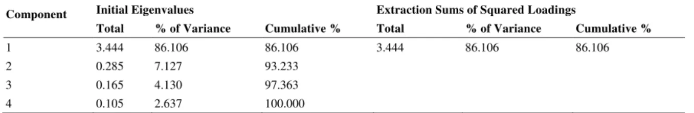
After testing the correlation among the variables, the second factor can be expressed as a linear combination of the candidate variables through PCA. Total variance explained is used to extract the principal factor. Extracted sums of loading is shown in Table II.
TABLE II
TOTAL VARIANCE EXPLAINED IN EXTRACTING NUMBER OF COMPONENT
Component Initial Eigenvalues Extraction Sums of Squared Loadings
Total % of Variance Cumulative % Total % of Variance Cumulative %
1 3.444 86.106 86.106 3.444 86.106 86.106 2 0.285 7.127 93.233
3 0.165 4.130 97.363 4 0.105 2.637 100.000
Usually more than one component is needed for the second factor. However, in this case, the first component has already explained 86.11% of the proportion of variance. Therefore, we choose only the first component as the second factor. Thus, the second factor is the absolute score value of the first principal component, which is denoted by |PRIN1|. Table III shows the component matrix generated through PCA.
USD/MYR USD/SGD USD/THB USD/IDR KLCI
USD/MYR Pearson Correlation 1 .906** .824** .801** -.571**
Sig. (2-tailed) .000 .000 .000 .000
USD/SGD Pearson Correlation 1 .887** .842** -.770**
Sig. (2-tailed) .000 .000 .000
USD/THB Pearson Correlation 1 .849** -.753**
Sig. (2-tailed) .000 .000
USD/IDR Pearson Correlation 1 -.773**
Sig. (2-tailed) .000
TABLE III
COMPONENT MATRIX OF THE SECOND FACTOR
Exchange Component 1
USD/SGD 0.947
USD/THB 0.943
USD/IDR 0.935
KLCI -0.885
Based on the result of principal component, the second factor can be written as | * KLCI 885 . 0 * IDR 935 . 0 * THB 943 . 0 * SGD 947 . 0 | | 1 PRIN | = • + • + • − •
where SGD*, THB*, IDR* and KLCI* are the values of USD/SGD, USD/THB, USD/IDR and KLCI after standardization via component matrix analysis respectively.
Values of the first and second factor are employed as the input data for the distance-based fuzzy time series forecasting.
Step 3: Divide the Universe of Discourse
Let U denote the universe of discourse of the first factor and V denote the universe of discourse of the second factor. For example, data of the exchange rate on 11 August 2009, Dmin = 3.4422, Dmax = 3.7276, D1 = 0, D2 = 0.0006, since U=[Dmin −D1,Dmax+D2]. Consequently, we have U = [3.4422, 3.7282]. Similarly, we have
Vmin = 0.04996751, Vmax = 6.43732423, V1 = 0, V2 = 0.01904328, since V=[Vmin −V1,Vmax +V2], thus
we have V = [0.04996751, 6.45636751]. Step 4: Define Fuzzy Sets
In this model, the first factor is divided into 286 equal length intervals with the length of each interval as 0.001. Similarly, the second factor is also divided into 286 equal length intervals, but with the length of each interval as 0.0224. The fuzzy sets of the first factor are partly represented as follows:
286 285 284 283 282 5 4 3 2 1 286 286 285 284 283 282 5 4 3 2 1 285 286 285 284 283 282 5 4 3 2 1 284 286 285 284 283 282 5 4 3 2 1 283 286 285 284 283 282 5 4 3 2 1 282 286 285 284 283 282 5 4 3 2 1 5 286 285 284 283 282 5 4 3 2 1 4 286 285 284 283 282 5 4 3 2 1 3 286 285 284 283 282 5 4 3 2 1 2 286 285 284 283 282 5 4 3 2 1 1
/
1
/
5
.
0
/
0
/
0
/
0
..
/
0
/
0
/
0
/
0
/
0
/
5
.
0
/
1
/
5
.
0
/
0
/
0
..
/
0
/
0
/
0
/
0
/
0
/
0
/
5
.
0
/
1
/
5
.
0
/
0
..
/
0
/
0
/
0
/
0
/
0
/
0
/
0
/
5
.
0
/
1
/
5
.
0
..
/
0
/
0
/
0
/
0
/
0
/
0
/
0
/
0
/
5
.
0
/
1
..
/
0
/
0
/
0
/
0
/
0
/
0
/
0
/
0
/
0
/
0
..
/
1
/
5
.
0
/
0
/
0
/
0
/
0
/
0
/
0
/
0
/
0
..
/
5
.
0
/
1
/
5
.
0
/
0
/
0
/
0
/
0
/
0
/
0
/
0
..
/
0
/
5
.
0
/
1
/
5
.
0
/
0
/
0
/
0
/
0
/
0
/
0
..
/
0
/
0
/
5
.
0
/
1
/
5
.
0
/
0
/
0
/
0
/
0
/
0
...
/
0
/
0
/
0
/
5
.
0
/
1
u
u
u
u
u
u
u
u
u
u
A
u
u
u
u
u
u
u
u
u
u
A
u
u
u
u
u
u
u
u
u
u
A
u
u
u
u
u
u
u
u
u
u
A
u
u
u
u
u
u
u
u
u
u
A
u
u
u
u
u
u
u
u
u
u
A
u
u
u
u
u
u
u
u
u
u
A
u
u
u
u
u
u
u
u
u
u
A
u
u
u
u
u
u
u
u
u
u
A
u
u
u
u
u
u
u
u
u
u
A
+
+
+
+
+
+
+
+
+
+
=
+
+
+
+
+
+
+
+
+
+
=
+
+
+
+
+
+
+
+
+
+
=
+
+
+
+
+
+
+
+
+
+
=
+
+
+
+
+
+
+
+
+
+
=
+
+
+
+
+
+
+
+
+
+
=
+
+
+
+
+
+
+
+
+
+
=
+
+
+
+
+
+
+
+
+
+
=
+
+
+
+
+
+
+
+
+
+
=
+
+
+
+
+
+
+
+
+
+
=
286 285 284 283 282 5 4 3 2 1 286 286 285 284 283 282 5 4 3 2 1 285 286 285 284 283 282 5 4 3 2 1 284 286 285 284 283 282 5 4 3 2 1 283 286 285 284 283 282 5 4 3 2 1 282 286 285 284 283 282 5 4 3 2 1 5 286 285 284 283 282 5 4 3 2 1 4 286 285 284 283 282 5 4 3 2 1 3 286 285 284 283 282 5 4 3 2 1 2 286 285 284 283 282 5 4 3 2 1 1
/
1
/
5
.
0
/
0
/
0
/
0
..
/
0
/
0
/
0
/
0
/
0
/
5
.
0
/
1
/
5
.
0
/
0
/
0
..
/
0
/
0
/
0
/
0
/
0
/
0
/
5
.
0
/
1
/
5
.
0
/
0
..
/
0
/
0
/
0
/
0
/
0
/
0
/
0
/
5
.
0
/
1
/
5
.
0
..
/
0
/
0
/
0
/
0
/
0
/
0
/
0
/
0
/
5
.
0
/
1
..
/
0
/
0
/
0
/
0
/
0
/
0
/
0
/
0
/
0
/
0
..
/
1
/
5
.
0
/
0
/
0
/
0
/
0
/
0
/
0
/
0
/
0
..
/
5
.
0
/
1
/
5
.
0
/
0
/
0
/
0
/
0
/
0
/
0
/
0
..
/
0
/
5
.
0
/
1
/
5
.
0
/
0
/
0
/
0
/
0
/
0
/
0
..
/
0
/
0
/
5
.
0
/
1
/
5
.
0
/
0
/
0
/
0
/
0
/
0
...
/
0
/
0
/
0
/
5
.
0
/
1
v
v
v
v
v
v
v
v
v
v
B
v
v
v
v
v
v
v
v
v
v
B
v
v
v
v
v
v
v
v
v
v
B
v
v
v
v
v
v
v
v
v
v
B
v
v
v
v
v
v
v
v
v
v
B
v
v
v
v
v
v
v
v
v
v
B
v
v
v
v
v
v
v
v
v
v
B
v
v
v
v
v
v
v
v
v
v
B
v
v
v
v
v
v
v
v
v
v
B
v
v
v
v
v
v
v
v
v
v
B
+
+
+
+
+
+
+
+
+
+
=
+
+
+
+
+
+
+
+
+
+
=
+
+
+
+
+
+
+
+
+
+
=
+
+
+
+
+
+
+
+
+
+
=
+
+
+
+
+
+
+
+
+
+
=
+
+
+
+
+
+
+
+
+
+
=
+
+
+
+
+
+
+
+
+
+
=
+
+
+
+
+
+
+
+
+
+
=
+
+
+
+
+
+
+
+
+
+
=
+
+
+
+
+
+
+
+
+
+
=
Step 5: Fuzzification
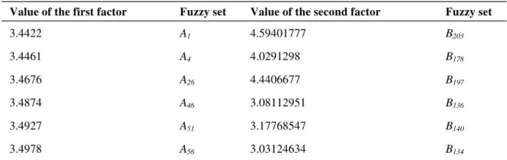
After defining the fuzzy sets, we fuzzify the historical data set of the first factor and the second factor. The fuzzy sets of the first factor and the second factor are partly shown in Table IV
TABLE IV
FUZZY SETS OF THE FIRST FACTOR AND THE SECOND FACTOR
Value of the first factor Fuzzy set Value of the second factor Fuzzy set
3.4422 A1 4.59401777 B203
3.4461 A4 4.0291298 B178
3.4676 A26 4.4406677 B197
3.4874 A46 3.08112951 B136
3.4927 A51 3.17768547 B140
3.4978 A56 3.03124634 B134
Step 6: Construct Fuzzy Logic Relationship (FLR) Database
After completing the process of fuzzification, we establish the FLR database. A sample of the FLRs’ database is written as
FLR1 : A1 B203 A4 B178 A26 B197
A46
FLR2 : A4 B178 A26 B197 A46 B136 A51
FLR3 : A26 B197 A46 B136 A51 B140 A56
FLR4 : A46 B136 A51 B140 A56 B134 A67
FLR5 : A51 B140 A56 B134 A67 B130 A71
FLR6 : A56 B134 A67 B130 A71 B84 A53
Step 7: Forecastingusing distance-based
The exchange rate of USD/MYR on 11 August 2009 is used as an example. (1) Construct the LHS of the FLR on 11 August 2009.
In this step, we first construct the LHS of the FLR on 11 August 2009 and then we use it to select the forecasting FLR rules from the FLRs database. The LHS of the FLR on 11 August 2009 is shown as follows:
(A49, B271), (A59, B261), (A63, B262). (2) Search for suitable forecasting FLR rules.
The k forecasting FLR rules are selected from the FLR database. In this model, k is set to 3 because we are doing the third-order model. The Euclidean distances (EDs) between the LHS of the FLR on 11 August 2009 and the FLRs from the FLR database are calculated. The ED denote the distance between the LHS on day t and the LHS of a candidate FLR rule on day i, then we have
=
− −
−
− − + −
=
n
1 j
2 j i j t 2 j i j
t RX ) (IY RY ) )
IX (( ED
where IXt−jandIYt−j are the subscripts of the fuzzy sets of the LHS of day t’s FLR, respectively; that
is IXt−j is the subscript of fuzzy set Xt−j and IYt−j is the subscript of fuzzy set Yt−j in the equation
)
Y
,
X
(
),
Y
,
X
(
...,
),
Y
,
X
(
t−n t−n t−2 t−2 t−1 t−1 . Similarly, RXi−jandRYi−j are the subscripts oftheir corresponding fuzzy sets at the LHS of day i's FLR. Here are some examples for the calculation of EDs:
For FLR1:
ED = 2 2 2 2 2 2
) 197 262 ( ) 26 63 ( ) 178 261 ( ) 4 59 ( ) 203 271 ( ) 1 49
( − + − + − + − + − + −
= 149.7865147
For FLR2:
ED =
2 2
2 2
2 2
) 136 262 ( ) 46 63 ( ) 197 261 ( ) 26 59 ( ) 178 271 ( ) 4 49
( − + − + − + − + − + −
= 178.9525077
The other EDs between the LHS of the FLR on 11 August 2009 are calculated with the similar manner. It is found that the 3 smallest EDs are FLR212, FLR211 and FLR210 where corresponding EDs are 16.7928, 22.3383 and 39.5979.
(3) Forecast the exchange rate on 11 August 2009
The exchange rate of USD/MYR can be forecasted by using the equation
=
=
k
1 j
] j [ M ] j [ ED
1 W
1 value _
forecast , where
=
=
k
1 j ED[j]
1
W ; ED[j] is the jth smallest Euclidean
distance; M[j] is the midpoint value of the fuzzy set at the RHS of the FLR with the j-th smallest Euclidean distance. If ED[j] = 0 for any j where1≤ j≤k, then the forecast value is equal to the average of M[j] whose corresponding ED[j] = 0. In this case study k equal to 3 as it takes third order fuzzy time series. The required information for forecasting is shown in Table V.
TABLE V
PREREQUISITE INFORMATION TO CALCULATE FORECASTED EXCHANGE RATE
FLR with the smallest EDs
ED RHS of the FLR Interval Range Midpoint
Value
FLR212 16.7928 A63 3.5042 3.5052 3.5047
FLR211 22.3383 A59 3.5002 3.5012 3.5007
FLR210 39.5979 A49 3.4902 3.4912 3.4907
Substitute ED[1] with 16.79285562, ED[2] with 22.3383079 and ED[3] with 39.59797975 into the weight function and we have
129569095 .
0 ] j [ ED
1 W
3
1 j
=
=
=
.
Similarly, substitute midpoint value into the equation
=
=
k
1 j
] j [ M ] j [ ED
1 W
1 value _
forecast . The forecasted
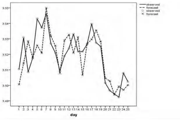
Fig. I . Trends Of The Usd/Myr Exchange Rates Forecasting Versus The Observed Rates
To check the accuracy of the prediction model, mean square error (MSE) is used. The MSE is calculated using the following formula.
n
∑n
1 = t
2 day t) on value g Forecastin
-day t on value (Actual =
MSE
A comparison of MSE between two different data sets under the same model was conducted. The forecasted exchange rates of USD/MYR and USD/NTD were compared in terms of MSE. The MSE for USD/NTD exchange rate forecasting was retrieved from [17]. A sample of one-day, three-day, five-day and seven-day forecasting based on forecasted rates of USD/MYR and USD/NTD was investigated. The results of MSE of exchange rate USD/MYR and USD/NTD for one-day, three-day, five-day and seven-day forecasting are shown in Table VI.
TABLE VI
Exchange rate forecasting errors for USD/MYR and USD/NTD
USD/MYR USD/NTD
MSE MSE
One-day 9.8 x10⁻⁵ 6.5 x 10⁻³
Three-day 3.9 x 10⁻⁴ 2.8 x 10⁻²
Five-day 2.9 x 10⁻⁴ 5.0 x 10⁻²
Seven-day 1.3 x 10⁻⁵ 5.3 x 10⁻²
As shown in Table VI , data sets of USD/MYR has smaller error than USD/NTD for the sample days of the forecasting. The errors indicate that the USD/MYR exchange rates are performed better than the USD/NTD.
IV.CONCLUSIONS
fuzzy time series. The model finally identified the forecasted value of USD/MYR exchange rate. The performance of the model in the case of exchange rate was measured using mean square error. As to check the performance compared with other exchange rate forecasting data, a comparison of mean square errors between USD/MYR and USD/ NTD were made. Under the same model, the errors for USD/MYR were smaller than the USD/NTD. It is concluded that the exchange rate forecasting for USD/MYR using the distance-based fuzzy time series is performed well when compared with USD/NTD data sets. However, the results were based solely on the selected model and not verified with other models. Perhaps the same datasets could also be tested to other models. Furthermore, the number of input data could also be increased as it would affect the forecasting accuracy. Other measure of accuracy such as mean absolute percentage error could also be tested. Extension of the present research is needed as to benchmark the forecasting results and reaffirm the feasibility of models in foreign exchange forecasting.
REFERENCES
[1] A.S. Chen and T. Leung . A Bayesian vector error correction model for forecasting exchange rates. Computer and Operations Research, vol.30, no.6, pp.887-900, 2003.
[2] C. Panda and V. Narasimhan . Forecasting exchange rate better with artificial neural network. Journal of Policy Modeling, vol. 29, no.2, pp. 227-236. 2007
[3] L. Anastasakis and N. Mort . Exchange rate forecasting using a combined parametric and nonparametric self-organising modelling approach. Expert Systems with Applications, vol.36, no.10, pp. 12001-12011. 2009
[4] Q.Song, and B.S. Chissom,. Fuzzy time series and its model. Fuzzy Sets and Systems, vol. 54, no. 3, pp. 269-277. 1993a
[5] Q .Song and B.S. Chissom. Forecasting enrollments with fuzzy time series - Part 1. Fuzzy Sets and Systems, vol. 54, no. 1, pp. 1-9. 1993b.
[6] Q. Song and B.S. Chissom,. Forecasting enrollments with fuzzy time series - Part 2. Fuzzy Sets and Systems, vol, 62, no. 1, pp. 1-8. 1994.
[7] S.M. Chen. Forecasting enrolments based on fuzzy time series. Fuzzy Sets and Systems, vol.81, no. 3, pp.311-319. 1996. [8] S.M. Chen. Forecasting enrolments based on high-order fuzzy time series. Cybernetics and Systems , vol.33, no. 1, pp.1-16. 2002. [9] R.C. Tsaur, J.C.O.Yang, and H.F. Wang. Fuzzy relation analysis in fuzzy time series model. Computer and Mathematics with
Applications vol. 49, no.4, pp.539–548. 2005.
[10] L. Abdullah and C.W. Loh. A Fuzzy Time Series Model in Forecasting Malaysian Government Direct Tax Collection. Proceedings of the Conference on Data Mining and Optimization, DOI: 10.1109/DMO.2009.5341913, pp. 42-45. 2009. Kuala Lumpur.
[11] L.Abdullah and Y.L. Chai. (). Intervals in Fuzzy Time Series Model: Preliminary Investigation for Composite Index Forecasting, ARPN Journal of Systems and Software, vol. 2, no. 1, pp. 7-11. 2012.
[12] L. Abdullah, and L.F. Fan. Fourth-order Fuzzy Time Series Based on Multi-Period Adaptation Models for Kuala Lumpur Composite Index Forecasting, Journal of Emerging Trends in Computing and Information Sciences, vol. 2, no. 1, pp. 16-20. 2011.
[13] L. Abdullah and Y.L. Chai A Fuzzy Time Series Model for Kuala Lumpur Composite Index Forecasting. IEEE Proceedings of Fourth International Conference on Modeling, Simulation and Applied Optimization,. DOI: 10.1109/ICMSAO.2011.5775515, pp.1-5. 2011, Kuala Lumpur
[14] S.M. Chen and J.R. Hwang. Temperature prediction using fuzzy time series. IEEE Transactions on Systems, Man, and Cybernetics – Part B: Cybernetics,vol.30, no. 2, pp. 263-275. 2000.
[15] L.W. Lee, L.H. Wang, S.M. Chen, and Y.H. Leu. Handling forecasting problems based on two-factor high-order fuzzy time series. IEEE Transactions on Fuzzy Systems, vol. 14, no. 3, pp.468–477. 2006.
[16] T.L. Chen, C.H.Cheng and H.J. Teoh. Fuzzy time series based on Fibonacci sequence for stock price forecasting. Physica A: Statistical Mechanics and Its Applications, vol. 380, pp. 377–390. 2007.