www.nonlin-processes-geophys.net/18/735/2011/ doi:10.5194/npg-18-735-2011
© Author(s) 2011. CC Attribution 3.0 License.
in Geophysics
Ensemble Kalman filtering without the intrinsic need for inflation
M. Bocquet1,2
1Universit´e Paris-Est, CEREA Joint Laboratory ´Ecole des Ponts ParisTech/EDF R&D, France 2INRIA, Paris Rocquencourt Research Center, France
Received: 8 August 2011 – Revised: 14 October 2011 – Accepted: 16 October 2011 – Published: 20 October 2011
Abstract. The mainintrinsicsource of error in the ensem-ble Kalman filter (EnKF) is sampling error. External sources of error, such as model error or deviations from Gaussianity, depend on the dynamical properties of the model. Sampling errors can lead to instability of the filter which, as a conse-quence, often requires inflation and localization. The goal of this article is to derive an ensemble Kalman filter which is less sensitive to sampling errors. A prior probability density function conditional on the forecast ensemble is derived us-ing Bayesian principles. Even though this prior is built upon the assumption that the ensemble is Gaussian-distributed, it is different from the Gaussian probability density function defined by the empirical mean and the empirical error co-variance matrix of the ensemble, which is implicitly used in traditional EnKFs. This new prior generates a new class of ensemble Kalman filters, called finite-size ensemble Kalman filter (EnKF-N). One deterministic variant, the finite-size en-semble transform Kalman filter (ETKF-N), is derived. It is tested on the Lorenz ’63 and Lorenz ’95 models. In this con-text, ETKF-N is shown to be stable without inflation for en-semble size greater than the model unstable subspace dimen-sion, at the same numerical cost as the ensemble transform Kalman filter (ETKF). One variant of ETKF-N seems to sys-tematically outperform the ETKF with optimally tuned in-flation. However it is shown that ETKF-N does not account for all sampling errors, and necessitates localization like any EnKF, whenever the ensemble size is too small. In order to explore the need for inflation in this small ensemble size regime, a local version of the new class of filters is defined (LETKF-N) and tested on the Lorenz ’95 toy model. What-ever the size of the ensemble, the filter is stable. Its perfor-mance without inflation is slightly inferior to that of LETKF with optimally tuned inflation for small interval between up-dates, and superior to LETKF with optimally tuned inflation for large time interval between updates.
Correspondence to:M. Bocquet
1 Introduction
The ensemble Kalman filter (EnKF) has become a very popu-lar potential substitute to variational data assimilation in high dimension, because it does not require the adjoint of the evo-lution model, because of a low storage requirement, because of its natural probabilistic formulation, and because it easily lends itself to parallel computing (Evensen, 2009 and refer-ence therein).
1.1 Errors in the ensemble Kalman filter schemes
The EnKF schemes can be affected by errors of different na-ture. A flaw of the original scheme (Evensen, 1994) which incompletely took into account the impact of the uncertainty of the observations in the analysis, was corrected by Burgers et al. (1998). They introduced a stochastic EnKF, by perturb-ing the observations for each member of the ensemble, in accordance with the assumed observational noise. Alterna-tives to the stochastic schemes are the deterministic ensem-ble Kalman filters introduced by Anderson (2001); Whitaker and Hamill (2002); Tippett et al. (2003).
Even with this correction, EnKF is known to often suffer from undersampling issues, because it is based on the ini-tial claim that the few tens of members of the ensemble may suffice to represent the first and second-order statistics of er-rors of a large geophysical system. This issue was diagnosed very early by Houtekamer and Mitchell (1998); Whitaker and Hamill (2002). Indeed, the failure to properly sample leads to an underestimation of the error variances, and ultimately to a divergence of the filter.
Adding to the error amplitude mismatch, undersampling generates spurious correlations, especially at long distance separation as addressed by Houtekamer and Mitchell (1998); Hamill et al. (2001).
1.2 Strategies to reduce error
Besides the early correction of the stochastic filter, tech-niques were devised to correct, or make up for the sampling issues. For both deterministic and stochastic filters, the er-ror amplitude problem can be fixed by the use of an inflation of the ensemble: the anomalies (deviations of the members from the ensemble mean) are scaled up by a factor that ac-counts for the underestimation of the variances (Anderson and Anderson, 1999; Hamill et al., 2001). Alternatively, the inflation can be additive via stochastic perturbations of the ensemble members, as shown by Mitchell and Houtekamer (1999); Corazza et al. (2002) where it was used to account for the misrepresented model error.
As far as stochastic filters are concerned, Houtekamer and Mitchell (1998, 2001) proposed to use a multi-ensemble configuration, where the ensemble is split into several sub-ensembles. The Kalman gain of one sub-ensemble can be computed from the rest of the ensemble, avoiding the so-called inbreeding effect. Remarkably, in a perfect model context, the scheme was shown to avoid the intrinsic need for inflation (Mitchell and Houtekamer, 2009).
Unfortunately, inflation or multi-ensemble configuration do not entirely solve the sampling problem and especially the long-range spurious correlations. These can be addressed in two ways under the name of localization. The first route con-sists in increasing the rank of the forecast error covariance matrix by applying a Schur product with a short-range ad-missible correlation matrix (Houtekamer and Mitchell, 2001; Hamill et al., 2001). The second route consists in making the analysis local by assimilating a subset of nearby observations (Ott et al., 2004 and references therein). Though vaguely connected, the two approaches still require common grounds to be understood (Sakov and Bertino, 2010). But alternative methods have emerged, either based on cross-validation (An-derson, 2007a), on multiscale analysis (Zhou et al., 2006), or on empirical considerations (Bishop and Hodyss, 2007).
Many of these techniques introduce additional parameters, such as the inflation factor, the number of sub-ensembles, or the localization length. A few of these parameters can even be made local. They can be chosen from experience gathered on a particular system, or they can be estimated online.
The online estimation methods are adaptive techniques, which is a growing subject. Focussing on the inflation issue, they are based on a specific maximum likelihood estimator of the inflation scaling, or of several scalars that parameter-ize the error covariance matrices (Mitchell and Houtekamer, 1999; Anderson, 2007b; Brankart et al., 2010) essentially following the ideas of Dee (1995). Another adaptive ap-proach (Li et al., 2009) use the diagnostics of Desroziers et al. (2005).
1.3 Towards objective identification of errors
More straightforward approaches have recently been ex-plored through the identification of the sampling errors. Mal-lat et al. (1998); Furrer and Bengtsson (2007); Raynaud et al. (2009) put forward a quantitative argument that shows the shortcomings of sampling. Let us define an ensemble ofN state vectorsxk inRM, fork=1,...,N. The empirical mean
of the ensemble is x= 1
N
N
X
k=1
xk, (1)
and the empirical background error covariance matrix of the ensemble is
P= 1
N−1
N
X
k=1
(xk−x)(xk−x)T. (2)
They assume that the ensemble members are drawn from a multivariate Gaussian distribution of unknown covariance matrix B, that generally differs from the empirically esti-mated covariance matrixP. Then the variance of each entry ofPcan be assessed using Wick’s theorem (Wick, 1950): E
[P−B]2ij
= 1
N
[B]ii[B]jj+ [B]2ij
, (3)
withi,j=1,...,M indexing the state space grid-cells; E is the expectation operator of the Gaussian process and [C]ij
generically denotes entry(i,j )of matrixC.
In particular one obtains the average of the error on the estimated variances inB
E[P−B]2ii= 2
N[B] 2
ii, (4)
which has been used in an ensemble of assimilations (Ray-naud et al., 2009). Considering covariances at long distance (i6=j),[B]ijis expected to vanish for most geophysical
sys-tems. And yet the errors in estimating[B]ij
E[P−B]2ij∼ 1
N[B]ii[B]jj, (5) are all but vanishing for a small ensemble. The impact of these errors on the analysis can be objectively estimated us-ing the results of van Leeuwen (1999); Furrer and Bengtsson (2007); Sacher and Bartello (2008).
This type of approach may offer objective solutions to ac-count for sampling errors. However incorporating them into data assimilation scheme is not straightforward. For instance, the objective identification of the covariance errors Eq. (3) depends on the true covariances, which are unknown, and some approximate closure is needed.
the propagation by a possibly nonlinear dynamical model. However this assumption allows to perform analytical com-putation using the properties of Gaussian distributions. Be-sides if the analysis of the data assimilation system only requires first- and second-order moments, higher-order mo-ments are irrelevant for the update, although certainly not for the global performance of a filter. Following these authors, we shall use this statistical assumption.
1.4 Objectives and outline
In the context of ensemble Kalman filtering, the first objec-tive of this article is to build a prior, to be used in the analysis step. Working on the first- and second-order empirical mo-ments of the ensemble, a traditional ensemble Kalman filter performs an update as if the prior distribution was given by a Gaussian defined by the empirical momentsxandP. Instead, our prior of the true state is conditioned on the entire forecast ensemble, not only its first- and second-order empirical mo-ments. Knowing about the discrete nature of the ensemble, it should partly or completely account for the sampling flaws.
Our goal is, within the framework of ensemble Kalman filtering, to perform a Bayesian analysis with this new prior. In Sect. 2, such a prior is derived.
The use of this prior in the analysis will result in the defini-tion of a new class of algorithms for high-dimensional filter-ing that are exploited in Sect. 3, the size (i.e. finite-sample) ensemble Kalman filters (denoted EnKF-N). We shall study one of its variant, which is an extension of the en-semble transform Kalman filter (ETKF) of Hunt et al. (2007), that we call the finite-size ensemble transform Kalman filter (ETKF-N).
In Sect. 4, the new filters are applied to the Lorenz ’63 and Lorenz ’95 models. Their performance is compared to ETKF. The new filters do not seem to require inflation. Un-fortunately, like any ensemble Kalman filter, ETKF-N di-verges for small ensemble sizes in the Lorenz ’95 case. It does require localization. This shows that the new filters do not entirely solve the sampling issue, and the reason for this is discussed in Sect. 5. Yet, a local variant of ETKF-N, the finite-size local ensemble transform Kalman filter (LETKF-N), can be built. It is tested on the Lorenz ’95 toy model, and compared to the local ensemble transform Kalman filter (LETKF). The main goal of introducing LETKF-N is to ex-amine whether the need for inflation is still avoided, in spite of the imbalance that localization is known to generate. In Sect. 6, the results are summarized. A few leads to go further are also discussed.
In this article, model error is not considered. It is assumed throughout this study that the model is perfect. Therefore, in this study, inflation is meant to compensate for sampling errors (hence the adjectiveintrinsicin the title). Theoreti-cally, (additive or multiplicative) inflation for model error is a rather distinct subject from inflation for sampling errors, even though it is difficult to untangle the two in practice.
The filters derived in this article should be applicable to (very) high-dimensional geophysical systems. This requires that only a small ensemble can be propagated between up-dates (typically no more than 100 members).
2 Accounting for sampling errors
We would like to reformulate the traditional analysis step of the EnKF. The prior (or previous forecast) is the focus of the reasoning. The prior that is usually used in the EnKF is given by the prior pdf of the state vector x, a vector in
RM, conditional on the empirical meanxand on the empiri-cal background error covariance matrixP, defined in Eqs. (1) and (2). Moreover this conditional pdf of the priorp(x|x,P) is implicitly assumed to be Gaussian. Lacking further infor-mation, it is the more natural distribution knowing its first-and second-order moments.
2.1 Getting more from the ensemble
Unfortunately, information is lost: this prior does not take into account the fact thatx andPoriginate from sampling. That is why we aim at computing the prior pdf ofx condi-tional on the ensemble,p(x|x1,...,xN). It is assumed that
the members of the ensemble are independently drawn from a multivariate Gaussian distribution of mean statexband
co-variance matrixB. As argued in the introduction this assump-tion leads to an approximaassump-tion, since the ensemble members are rather samples of a (more or less) non-Gaussian distribu-tion (Bocquet et al., 2010; Lei et al., 2010). There is no point in modelling higher-order moments of the statistics prior to the analysis, since the analysis of the Kalman filter only uses the first- and second-order moments. The momentsxb and
Bof the true sampled distribution are unknown a priori and may differ fromxandP.
Summing over all potentialxbandB, whereBis a positive
definite matrix, the prior pdf reads p(x|x1,...,xN)
= Z
dxbdBp(x|x1,...,xN,xb,B)p(xb,B|x1,...,xN) =
Z
dxbdBp(x|xb,B)p(xb,B|x1,...,xN). (6)
The symbol dBcorresponds to the Lebesgue measure on all independent entries QMi≤jd[B]ij, but the integration is
re-stricted to the cone of positive definite matrices. From the first to the second line, we used the fact that under the as-sumption of Gaussianity of the prior pdf of the errors, the conditioning ofp(x|x1,...,xN,xb,B)on the ensemble is
re-dundant, since the pdf is completely characterized byxb, and
p(x|x1,...,xN)=
1 p(x1,...,xN)
× Z
dxbdBp(x|xb,B)p(x1,...,xN|xb,B)p(xb,B). (7)
The probability densities that are conditional on xb andB
can be written explicitly thanks to the Gaussian assumptions. The first one in Eq. (7) would be the prior ofx, if one knew the exact mean and error covariance matrix. The second one is the likelihood of the members to be drawn from the Gaus-sian distribution of the same mean and error covariance ma-trix (similarly to Dee, 1995). The third pdf in the integral of Eq. (7) is a prior on the background statistics (anhyperprior) whose choice will be discussed later. Writing explicitly the two Gaussian pdfs in the integral of Eq. (7) and re-organizing the terms, one gets
p(x|x1,...,xN)∝
Z
dxbdBexp(−L(x,xb,B))p(xb,B),(8)
where
L(x,xb,B)=
1
2(x−xb)
TB−1(x−x b)+
1
2(N+1)ln|B|
+1
2
N
X
k=1
(xk−xb)TB−1(xk−xb), (9)
where|B|denotes the determinant ofB.
2.2 Choosing priors for the background statistics
For the filters designed in this article, like for any (very) high-dimensional ensemble-based Kalman filters, information on the background error statistics can only be transported by the ensemble between analyzes. Passing along information on the full statistics of the errors requires too much storage. That is one reason why the EnKF was preferred over the imprac-tical extended Kalman filter. Still, we have to make a priori assumptions on (the statistics of)xbandB.
The most popular one in multivariate statistics is Jeffreys’ prior. It maximizes the information that will be gained in any subsequent analysis made with that prior (making it as much less informative as possible). It is known that Jeffrey’s prior for the couple(xb,B)is not satisfying in practice, and one
should make the independence assumption (Jeffreys, 1961): p(xb,B)≡pJ(xb,B)=pJ(xb)pJ(B) (10) and compute the Jeffreys’ priors forxbandBseparately.
Jef-freys’ choice corresponds to pJ(xb)=1, pJ(B)= |B|−
M+1
2 , (11)
whereM is the dimension of the state space. The fact that pJ(xb,B)cannot be normalized is not truly an issue, like for
any non-informative priors in Bayesian statistics, provided
(as far as we are concerned) that integral Eq. (7) is proper. The prior ofBhas some important properties that are essen-tial for this study. First, it is invariant by any reparameteriza-tion of state vectors. Consider the change of state variables x=Fx′, whereFis a non-singular matrix in state space. It translates to B=FB′FT for the error covariance matrices. The Jacobian of this change of variables for B is (see for instance Muirhead, 1982)
dB= |F|M+1dB′, (12)
so that
pJ(B)dB= |FB′FT|− M+1
2 |F|M+1dB′=pJ(B′)dB′. (13) This justifies the power(M+1)/2. Besides we want the hy-perprior to lead to asymptotic Gaussianity: in the limit of a large ensemble, this choice should lead to the usual Gaussian prior used in EnKF analysis. This will be checked in Sect. 3. 2.3 EffectiveJbfunctional
Choosing the priorp(xb,B)≡pJ(xb)pJ(B), the integration onxbin Eq. (8) is straightforward and leads to
p(x|x1,...,xN)∝
Z
dBexp(−J(x,B)) , (14) where
J(x,B)=1
2 N
N+1(x−x)
TB−1(x−x)
+N+M+1
2 ln|B| + 1 2
N
X
k=1
(xk−x)TB−1(xk−x). (15)
This functional can be compactly written as
J(x,B)=1
2Tr
AB−1+N+M+1
2 ln|B|, (16)
where A= N
N+1(x−x)(x−x)
T+(N−
1)P. (17)
Like for most ensemble Kalman filters, especially ensemble transform Kalman filters, it is assumed in the following that x−xbelongs to the vector spaceVspanned by the anomalies xk−x. Because in the context of high-dimensional Kalman
filteringAis rank-deficient
rank(A)≤N−1≪M , (18)
matrices will produce an infinite volume factor with no de-pendence onx, that can be subtracted from the final effective functional. On more rigorous grounds, one can extend matrix Ato a full rank positive definite matrixAǫ=A+ǫIM, where
IM is the identity matrix of state space, andǫ >0. Then the
integral in Eq. (14) becomes proper. After the integration, one can letǫgoes to 0. A diverging term depending on ǫ only, and hence of no interest, can then be safely ignored.
To perform the integration on B in Eq. (14), one can proceed to the change of variables B=A1ǫ/2A1ǫ/2. From
Eq. (12), the Jacobian of this change of variable is dB= |Aǫ|
M+1
2 d. (19)
Therefore, the dependence inxthroughAǫ can be extracted
from the integral: p(x|x1,...,xN)
∝ |Aǫ|−N/2
Z
d||−(N+M+1)/2exp
−1
2Tr
−1
∝ |Aǫ|−N/2∝ |A|−N/2. (20)
It is important to realize that the last determinant ofA ac-tually applies to the restriction of the linear operator repre-sented byAin the canonical basis of subspaceV, which is of dimension lower or equal toN−1, and is, by this definition, not singular.
From the expression of p(x|x1,...,xN), we deduce the
background functional to be used in the subsequent analysis of our variant of the EnKF:
Jb(x)= −lnp(x|x1,...,xN)=
N
2 ln|A| +Cst
= N
2 ln
N
N+1(x−x)(x−x)
T+(N− 1)P
, (21)
up to some irrelevant constant. Let us remark that the mean of the ensemblexis the mean and mode ofp(x|x1,...,xN).
2.4 AlternateJbfunctional
One can argue against the choice ofpJ(xb)=1. It might be
considered too weakly informative. However as an hyper-prior, it provides information before the observation, but also before exploiting the ensemble. So, whatever information is passed on to the subsequent analysis, it is weak, unless the information content of the ensemble is weak and the obser-vation are not dense (small ensemble size, sparse/infrequent observation).
One alternative to the uniform distribution is to use a cli-matology forxb. It is not tested in this study. However it was
recently demonstrated in the context of ensemble Kalman fil-tering that such an approach is helpful for sparsely observed systems (Gottwald et al., 2011). Another alternative is to make specific choices forxb. Equation (6)
p(x|x1,...,xN)= Z
dxbdBp(x|xb,B)p(xb,B|x1,...,xN), (22)
would be affected in the following way. The probability den-sity p(x|xb,B) is conditional on the knowledge of B and
xb. For this density, we additionally assume a great
confi-dence inx, like any standard EnKF, so that the first guess xbof the sampled prior is believed to be very close toxand
p(x|xb,B)≃p(x|x,B). This assumption can be wrong for
small ensemble size. Therefore: p(x|x1,...,xN)
≃ Z
dBp(x|x,B)
Z
dxbp(xb,B|x1,...,xN). (23)
The rest of the derivation is fundamentally unchanged. The final background functional reads
Jbalt(x)=N
2 ln
(x−x)(x−x)T+(N−1)P
. (24)
However the disappearance of theN/(N+1)factor is not cosmetic, and may have consequences that are investigated later.
3 Finite-size ensemble transform Kalman filter
BecauseJb andJbalt are not quadratic, it is clear that the analysis should be variational, in a similar flavor as the max-imum likelihood ensemble filter (Zupanski, 2005; Carrassi et al., 2009). As such it can accommodate nonlinear observa-tion operators. Therefore, in this study, the analysis step will be variational, similarly to 3D-Var. One should minimize the cost function
Ja(x)=Jo(x)+Jb(x), (25)
with
Jo(x)=1
2(y−H (x))
TR−1(y−H (x)) ,
(26) wherey is the observation vector in observation space Rd, Ris the observation error covariance matrix, andH is the observation operator.
We shall call finite-size (or finite-sample) ensemble Kalman filters (EnKF-N), the ensemble Kalman filters that could be generated using this type ofJbterm in the analysis
step of the filter. In the following, the focus will be on the ensemble transform Kalman filter (ETKF) variant, following Hunt et al. (2007). The analysis is expressed as an element of subspacex+V. The state vector is characterized by a set of (redundant) coordinates{wk}k=1,...,N in the ensemble space:
x=x+ N
X
k=1
wk(xk−x). (27)
IfXk=xk−x are the anomalies, andXthe matrix of these
anomalies,X=(X1,...,XN), thenx−x=Xw. Hence, one
has A= N
N+1Xww
Recall that|A|represents the determinant of the linear oper-ator related toAbut restricted to subspace V. In the same subspace, the linear operator related toXXTis invertible, of inverse denoted XXT−1. One gets
|A| =
N N+1Xww
TXT+XXT
= XXT IV+
N N+1
XXT−1XwwTXT
∝1+ N
N+1w
TXTXXT−1Xw.
(29) There is a subtlety that we need to develop on, and which generalizes the clear explanation given by Hunt et al. (2007). 3.1 Gauge-invariance of the parameterization
As a family of vectors, the anomalies are not indepen-dent sincePNk=1Xk=0. Therefore parameterizingJb(x)= Jb(x+Xw)withwentails a so-calledgauge invariance (a redundancy inw): Jb(x+Xw)is invariant under a shift of allwkby a same constant. The number of degrees of freedom
of this invariance is given by the dimension of the kernel of X, which is at least one according to the previous remark.
The expression given by Eq. (29) is not invariant under ro-tations ofw. We could make it invariant by using the freedom of the gauge invariance. We can fix this gauge by choosing to minimize the cost function over thewthat have a null or-thogonal projection on the kernel ofX:
IN−XT
XXT
−1 X
w=0. (30)
With this constraint, |A| is proportional to 1+NN+1wTw. This is cumbersome to enforce though. Instead, to perform the same task, a gauge-fixing term
G(w)= N
N+1w T
IN−XT
XXT −1 X w, (31)
is inserted into the cost function Eq. (25)
Ja(x)=Jo(x)+N
2ln(|A|) , (32)
yielding an augmented cost function
e
Ja(w)=Jo(x+Xw)+N
2 ln(|A| +G(w)) . (33) For instance, in the case where rank(A)=N−1, one has
G(w)= 1
N+1
N
X
k=1 wk
!2
. (34)
Because ln is a monotonically increasing function, one gets
e
Ja(w)≥Ja(x+Xw), for allwinRN, with equality if and only ifG(w)=0. Moreover, for anyx there is aw⋆ in the kernel of X(G(w⋆)=0) such thatJa(x)=Jea(w⋆). As a
consequence, the two cost functionsJea(w)andJa(x)have the same minimum. Note that this implies that at the mini-mumwaofJea, one hasG(wa)=0.
Hence, instead of Eq. (25) one can use the cost function with a gauge-fixing term:
e
Ja(w)=1
2(y−H (x+Xw))
TR−1(y−H (x+Xw))
+N
2ln
1+ 1
N+w Tw
. (35)
Cost function Eq. (35) is not necessarily convex because the ln function is concave. Let us assume a linear observation op-erator, or linearized around the innovationy−H (x). Then a minimum always exists since for a linear observation opera-tor,Jo(x)is convex inw, and
e
Jb(w)=N
2 ln
1+1
N+w Tw
, (36)
is a monotonically increasing function when the norm ofw goes to infinity. Conversely, the cost function may have sev-eral minima (see Appendix A). As a consequence the nature of the minimizer, as well as the first guess of the iterative op-timization, may have an impact on the result. The first guess of the iterative minimization was chosen to bew=0, which favors the prior against the observation if several minima do exist. Even though it may sound wiser to favor observation, the choicew=0is clearly simpler.
3.2 Posterior ensemble
Oncewais obtained as the minimizer of Eq. (35), the
poste-rior state estimate is given by
xa=x+Xwa. (37)
We wish to compute a local approximation of the error co-variances at the minimum. The Hessian ofJebcan be com-puted in ensemble space:
e
Hb= ∇w2Jeb(w)=N
1+N1 +wTw
IN−2wwT
1+N1+wTw2
. (38)
The Hessian of the observation term is
e
Ho= ∇w2Jo(x+Xw)=(HX)TR−1HX, (39)
whereHis the tangent linear ofH. The analysis error covari-ance matrixePain ensemble space is approximately obtained
from the inverse matrix of the total Hessian at the minimum
ePa≃He−a1, (40)
whereHea=Heb(wa)+Heo(wa). Note thatHeamust be posi-tive definite by construction, even thoughHeb(wa)is not nec-essarily so.
ensemble anomalies, in ensemble space, are given by the columnsWak of the transform matrix
Wa= (N−1)ePa
1/2
U, (41)
whereUis an arbitrary orthogonal matrix that preserves the ensemble mean:Uu=uwhereu=(1,...,1)T. The degrees of freedom introduced byUallow to span the ensemble space of any ensemble square root Kalman filter (Sakov and Oke, 2008). Accordingly, the posterior ensemble in state space is given fork=1,...,Nby
xak=xa+XWak. (42) Let us check that the posterior ensemble is centered on xa. To do so, one has to verify thatu is in the kernel of XWa. If we can prove thatuis an eigenvector ofePa, then
XWau∝Xu=0. The eigenvectors ofePa are those of the
Hessian Hea at the minimum. SinceJo(x+Xw)is gauge invariant, it is easy to check thatu is in the kernel of the HessianHeo. (Note that this remark also applies without ap-proximation to nonlinear observation operators.) As forJeb
whose gauge-invariance has been intentionally broken, the argument cannot apply. But it was seen earlier that at the minimumG(wa)=0. In particular, one hasuTwa=0. As a consequence, it is clear from Eq. (38) thatuis an eigenvector ofHeb, of eigenvalueN (1+1/N+(wa)Twa)−1. Therefore the posterior ensemble is centered onxa. This property is
important for the consistency and ultimately the stability and performance of the filter (Wang et al., 2004; Livings et al., 2008; Sakov and Oke, 2008).
The new filters are based on several mild approximations that are imposed by the non-Gaussianity of the prior. Firstly, one might not sample the right minimum when there are sev-eral of them (see Appendix A). Or the right estimator could be the average rather than a mode of the posterior pdf. Sec-ondly, and unlike the Gaussian case, the inverse Hessian is only a local approximation of the analysis error covariance matrix (Gejadze et al., 2008).
3.3 Asymptotic Gaussianity
When the ensemble size goes to largeN→ ∞, the ln term in the background part of cost function Eq. (36), must decrease to smaller, yet always positive, values. So shouldε≡wTw=
PN
k=1wk2. Therefore, in this limit, one has
e
Jb=N
2 ln
1+ 1
N+w Tw
≃1
2+ N−1
2 w
Tw+ON−1,N−1ε,ε2,
(43) and the ETKF of Hunt et al. (2007) is recovered (assuming Uis the identity matrix).
3.4 Algorithm
The variant of the finite-size EnKF that has just been de-scribed is the finite-size ensemble transform Kalman filter (ETKF-N). The numerical implementation is similar to that of Harlim and Hunt (2007) (see Algorithm 2). The pseudo-code for ETKF-N is:
1. Obtain the forecast ensemble {xk}k=1,···,N from the
model propagation of the previous ensemble analysis. 2. Form the meanx, and the anomaly matrixX, necessary
for the evaluation of cost function Eq. (35).
3. Minimize cost function Eq. (35) iteratively starting with w=0, to obtainwa.
4. Compute xa and the Hessian Hea, from Eq. (37),
Eq. (38), and Eq. (39).
5. ComputeWa= Hea/(N−1)−1/2U. 6. Generate the new ensemble:xak=xa+XWak.
The complexity is the same as that of ETKF. The mini-mization of the analysis cost function, which is already well conditioned by construction, might be longer in such non-quadratic, and even non-convex context. However, the mini-mization remains in ensemble space, and is almost negligible in cost for high-dimensional applications with an ensemble size in the range of 10–100.
3.5 Interpretation
The influence of the background term of the cost func-tion,Jeb=N2ln 1+1/N+wTw, within the full cost func-tion Eq. (35), is compared to its counterpart in ETKF,Jeb=
N−1
2 w
Tw. Firstly, let us assume that the innovation is such
that, in the ETKF system, the analysis is driven away from the ensemble mean:
wTw= N
X
k=1
w2k≥O(1). (44)
In the ETKF-N system, the constraint enforced by the back-ground term would be alleviated by the presence of the ln function. Therefore, in the same situation (same innova-tion), ETKF-N would be more controlled by the observation than ETKF. In particular, larger deviations from the ensem-ble mean would be allowed. It is reminiscent of the way the Huber norm operates (Huber, 1973).
Secondly, assume that the innovation drives the ETKF sys-tem towards an analysis close to the ensemble mean wTw=
N
X
k=1
w2k≪1. (45)
function, the prior term cannot vanish even when the ensem-ble mean is taken as the optimal state. This is confirmed by the inverse of the HessianHeb, the contribution of the prior to
ePa, which isN−1(1+1/N )atwa=0, instead ofN−1. This
also corresponds to the residual 1/2 term inJebof Eq. (43). Algebraically, this offset comes in the formula by the inte-gration onxb: thisblurringtells the system not to trust the
ensemble mean entirely at finiteN.
We believe this is the same term 1+1/N that was diag-nosed by Sacher and Bartello (2008), who showed that, for a Gaussian process, the dispersion of the ensemble around the mean of the Gaussian should be(1+1/N )P, instead ofP, because the ensemble mean does not coincide with the mean of the Gaussian distribution.
3.6 Alternate ETKF-N
The alternative formulation of ETKF-N, that assumes x is the best estimator for the prior, leads to the background term
e
Jbalt=N
2ln
1+wTw. (46)
The only difference is in the missing 1/N offset term, which is not surprising since it was identified as a measure of the mistrust in the ensemble mean to represent the true forecast mean.
4 Tests and validation with simple models
In this section, the new filters will be numerically tested, on a three-variable chaotic dynamical toy model, as well as a one-dimensional chaotic dynamical toy model. For the numerical experiments,Uis chosen to be the identity.
4.1 Lorenz ’63 toy-model
4.1.1 Setup
The Lorenz ’63 model (Lorenz, 1963) is a model withM=3 variables, defined by the equations:
dx
dt =σ (y−x) dy
dt =ρx−y−xz dz
dt =xy−βz. (47)
The parameters are set to the original values (σ,ρ,β)=
(10,28,8/3), which are known to lead to chaotic dynamics, with a doubling time of 0.78 time units. In the following simulations, a reference simulation stands for the truth. The model is considered to be perfect: the model of the truth is the same as the one used in data assimilation runs. We gener-ate synthetic observations from the reference simulation for the three variables each 1t time interval, with 1t=0.10,
3 4 5 6 7 8 9
Ensemble size
1 2
0.5 1.5 2.5
Average analysis rmse
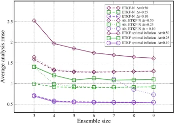
ETKF-N ∆t=0.50 ETKF-N ∆t=0.25 ETKF-N ∆t=0.10 Alt. ETKF-N ∆t=0.50 Alt. ETKF-N ∆t=0.25 Alt. ETKF-N ∆t = 0.10 ETKF optimal inflation ∆t=0.50 ETKF optimal inflation ∆t=0.25 ETKF optimal inflation ∆t=0.10
Fig. 1. Time-averaged analysis rmse for ETKF, ETKF-N and the al-ternate ETKF-N, for three experiments with different time intervals between updates, and for an ensemble size fromN=3 toN=9.
1t=0.25 and 1t=0.50. These choices are expected to generate mild, medium and strong impact of non-linearity and, as a possible consequence, non-Gaussianity of errors. These observations are independently perturbed with a nor-mal white noise of standard deviation 2 following Harlim and Hunt (2007). In comparison, the natural variability (standard deviation from the mean of a long model run) of the x, y, and z variables is 7.9, 9.0, and 8.6 respectively.
All the simulations are run for a period of time correspond-ing to 5×10⁵cycles, for the three values of1t. We use a burn-in period of 104cycles to minimize any impact on the final result. The ensemble size is varied fromN=3 toN=9. The filters are judged by the time-averaged value of the root mean square error between the analysis and the true state of the reference run.
4.1.2 Best rmse
For ETKF, a multiplicative inflation is applied by rescaling of the ensemble deviations from the mean:
xk−→x+r (xk−x) , (48)
so thatr=1 means no inflation. A wide range of inflation factorsris tested. The inflation factor leading to the smallest (best) rmse is selected. For finite-size filters, inflation is not considered. Therefore for each finite-size filter score, only one run is necessary.
The results are reported in Fig. 1.
of the true error distribution. For1t=0.25 and1t=0.50, where the errors are larger and the estimation ofxbmay be
relatively less important, the performance is almost as good as ETKF-N, with slight deviations for the smallest ensem-bles.
To a large extent, these results are similar to those of Har-lim and Hunt (2007). However, even though getting better results than ETKF, their filter still necessitates to adjust one parameter.
4.2 Lorenz ’95 toy-model
4.2.1 Setup
The filters are also applied to the one-dimensional Lorenz ’95 toy-model (Lorenz and Emmanuel, 1998). This model rep-resents a mid-latitude zonal circle of the global atmosphere, discretized intoM=40 variables{xm}m=1,...,M. The model
reads, form=1,...,M, dxm
dt =(xm+1−xm−2)xm−1−xm+F , (49) whereF =8, and the boundary is cyclic. Its dynamics is chaotic, and its attractor has a topological dimension of 13, a doubling time of about 0.42 time units, and a Kaplan-Yorke dimension of about 27.1.
The experiments follow the configuration of Sakov and Oke (2008). In the first experiment, the time interval between analyzes is1t=0.05, representative of time intervals of 6 hours for a global meteorological model. With this choice, non-linearity mildly affects the dynamics between updates. All variables are observed every1t. Therefore, the observa-tion operator is the identity matrix. All observaobserva-tions, which are obtained from a reference model run (the truth), are per-turbed with a univariate normal white distribution of stan-dard deviation 1. The observation error prior is accordingly a normal distribution of error covariance matrix the identity. In comparison, the natural variability of the model (standard deviation from the mean) is 3.6 for any of theM=40 vari-ables. The performance of a filter is assessed by the root mean square error (rmse) of the analysis with the truth, aver-aged over the whole experiment run.
As a burn-in period, 5×10³ analysis cycles are used, whereas 104analysis cycles are used for the assimilation ex-periments. This may be considered relatively short. How-ever, on the one hand, the convergence was deemed suffi-cient for this demonstrative study. On the other hand, about 5×10⁴ assimilation experiments have been performed, be-cause the inflation (and later the localization) parameters are investigated for many sizes of the ensemble. Longer runs (105analysis cycles) have also been performed, but no (long-term) instability was noted. Moreover these tests showed that the rmses of the 104-cycle cases had reasonably converged.
4.2.2 Ensemble size – inflation diagrams
Following Sakov and Oke (2008) and many others, we inves-tigate the rmse of the analysis with the reference state (the truth). The ensemble size is varied from 5 to 50. A mul-tiplicative inflation is applied by rescaling of the ensemble deviations from the mean according to Eq. (48). The infla-tion factorr is varied from 1.to 1.095 by step of 0.005. As a result, one obtains two-dimensional tables of rmse, which are displayed graphically.
The results for ETKF are reported in Fig. 2a. They are sim-ilar to the symmetric ensemble square root Kalman filter of Sakov and Oke (2008). The filter starts converging when the ensemble size is larger than the model unstable subspace di-mension. Inflation is always necessary, even for a size of the ensemble greater than the Kaplan-Yorke dimension pointing to a systematic underestimation of sampling errors.
The results of ETKF-N are reported on Fig. 2b. At first, it is striking that the filter diverges for ensemble sizes below N=15. This is disappointing, since the original goal of this study was to remedy to all sampling flaws in a deterministic context. This is obviously not achieved, similarly to any kind of EnKF without localization. However, the formalism de-veloped here allows to understand the reason of this failure, and how it could later be amended. This will be discussed in Sect. 5.
BeyondN=15 (which corresponds to a rank of 14 or less from the anomaly subspace, close to the model unstable sub-space dimension), the filter is unconditionally stable.
The results of the alternate ETKF-N are also reported on Fig. 2c. It is also unconditionally stable beyondN=15, but the rmses are better.
4.2.3 Best rmse
In the case of ETKF, the best root mean square error is ob-tained by taking, for each ensemble size, the minimal rmse over all inflation factors. For ETKF-N, there is only one rmse, since inflation is not considered. In Fig. 3 are plot-ted the best rmses for the three filters. The alternate ETKF-N seems to outperforms ETKF slightly. But its major asset is that the alternate ETKF-N obtains the best rmses without in-flation.
Both ETKF-N and alternate ETKF-N perform better than ETKF over the range N=5–16, especially in the critical rangeN=14–16. This has been checked for other config-urations (changingMandF) of the Lorenz ’95 model.
5 6 7 8 9 10 11 12 13 14 15 16 17 18 19 20 25 30 35 40 45 50 1.0
1.0051.01 1.0151.02 1.0251.03 1.0351.04 1.0451.05 1.0551.06 1.0651.07 1.0751.08 1.0851.09 1.095
Inflation factor
(a) ETKF
5 6 7 8 9 10 11 12 13 14 15 16 17 18 19 20 25 30 35 40 45 50
Ensemble size
0.95 0.9550.96 0.9650.97 0.9750.98 0.9850.99 0.9951.0 1.0051.01 1.0151.02 1.0251.03 1.0351.04 1.0451.05 1.0551.06 1.0651.07 1.0751.08 1.0851.09 1.095
Inflation factor
(b) ETKF-N
5 6 7 8 9 10 11 12 13 14 15 16 17 18 19 20 25 30 35 40 45 50
Ensemble size
1.0 1.0051.01 1.0151.02 1.0251.03 1.0351.04 1.0451.05 1.0551.06 1.0651.07 1.0751.08 1.0851.09 1.095
Inflation factor
(c) Alt. ETKF-N
0.18 0.19 0.20 0.21 0.22 0.23 0.24 0.25 0.26 0.27 0.28 0.29 0.30 0.31 0.32 0.33 0.34 0.35 0.36
Fig. 2. Root mean square errors of ETKF(a), ETKF-N(b), and alternate ETKF-N(c), for a wide range of ensemble size (5–50) and inflation parametersr=1,1.005,...,1.095 and in panel(b)a larger range of inflation/deflationr=0.945,...,1.095.
case for small1t, the forecasted ensemble will remain cen-tered on the trajectory of the mean, so that the mean of the ensemble will remain a good estimate of the true distribution mean. Therefore, the alternate ETKF-N, as well as symmet-ric ensemble square root filters, have an advantage in linear conditions over the more conservative, too cautious ETKF-N. If this is correct, then the performance of ETKF-N (which is symmetric) should be better, or at worst equal to the per-formance of a non-symmetric ensemble square root Kalman filter for small1t. Indeed this can be checked by compari-son of Fig. 3 of the present article and Fig. 4 of Sakov and Oke (2008). Moreover, according to this argument, the per-formance of ETKF-N should improve for larger ensemble size and larger1t, in comparison with ETKF (with optimal inflation).
As mentioned earlier, the time interval between updates has been set to1t=0.05. We know from the experiment on
the Lorenz ’63 model and from the previous remark, that the performance of ETKF-N as compared to ETKF is susceptible to vary with1t. Let us take the example of an ensemble size ofN=20. The setup is unchanged except for the time interval which is set to1t=0.05,0.10,...,0.30.
As shown in Fig. 4,1t≤0.15 is a turning point beyond which ETKF-N obtains better rmse than ETKF without in-flation. The alternate ETKF-N offers the best of ETKF (with optimal inflation) and ETKF-N, over the full range of1t.
5 Local extension of ETKF-N
5.1 Can the use of localization be avoided?
5 10 15 20 25 30 35 40 45 50
Ensemble size
0.2 0.3 0.4 0.5 1 2 3 4 5
Average analysis rmse
ETKF (optimal inflation) ETKF-N
Alt. ETKF-N
Fig. 3. Best rmse over a wide range of inflation factors for ETKF, and rmse without inflation for N and for the alternate ETKF-N.
of ETKF-N Eq. (35) is formulated in ensemble space, via a set of ensemble coordinates that do not depend on the real space position. This functional form is due to the choice of the Jeffrey’s prior. It implies that the dimension of the anal-ysis space has a very reduced rank. Localization, which is meant to increase this rank, is therefore mandatory below some context-dependent ensemble size. We could contem-plate two ways to tackle this difficult problem.
The first one would consist in trading Jeffrey’s prior for a more informative one. The particular form of the ETKF-N background term which depends only on the ensemble co-ordinates was due to the specific choice of Jeffrey’s prior, which had the merit to be simple. However, errors of the Lorenz ’95 data assimilation system, or of more realistic geo-physical systems, often have short-range correlations. If, us-ing an hyperprior different from Jeffreys’, one could inte-grate on a restricted set of error covariance matrices of cor-relation matching the climatological corcor-relations of the data assimilation system, we conjecture that localization could be consistently achieved within the proposed formalism.
Let us take an example where it is assumed that the corre-lations of the data assimilation system are very short-range. At the extreme, we integrate Eq. (14) on the set of all posi-tive definite diagonal matricesB, that is a set ofMpositive scalars, with the non-informative univariate prior:
pJ([B]ii)= [B]−ii1. (50)
Following the derivation of Sect. 2, one obtains
Jb(x)=N
2
M
X
i=1 ln
"
N
N+1(xi−xi) 2+
N
X
k=1
(xik−xi)2
#
. (51)
As opposed to the background terms introduced earlier, this
Jbcannot be written in ensemble space, i.e. not in terms of
0.05 0.10 0.15 0.20 0.25 0.30
Time interval between updates ∆t
0.20 0.30 0.40 0.50 0.60 0.70 0.80 0.90
Average analysis rmse
ETKF (optimal inflation) ETKF-N
Alt. ETKF-N
Fig. 4. Best rmse for ETKF over a wide range of inflation factors, rmse of N without inflation and rmse of the alternate ETKF-N without inflation, for several time intervals between updates, and for an ensemble sizeN=20.
the coordinates wk in the vector space of anomalies.
As-suming the same setup used for the Lorenz ’95 model, the average analysis rmse of such EnKF-N is in the range 0.50 forN=5 down to 0.35 forN=40. It has been checked to be similar to any EnKF or ETKF with a minimal (meaningful) localization length, except that, for this new filter, inflation is not necessary even for smallN. We conclude that localiza-tion can potentially be expressed in the formalism. Pursuing this idea is well beyond the scope of this article, because it seems mathematically challenging.
As an alternative, simpler, and widespread solution, a lo-cal version of the filter will be developed and tested in the remaining of this section.
5.2 LETKF-N
5.3 Application to the Lorenz ’95 toy-model
5.3.1 Ensemble size – inflation diagrams
The results of the experiments with LETKF, LETKF-N, and with the alternate LETKF-N are reported in Fig. 5.
For LETKF, inflation is still necessary to stabilize the filter for not-so-small ensemble sizes (N≤11). LETKF-N does not require inflation (at least forN≥5, the caseN <4 was not investigated). Again, it means that LETKF-N estimates well, or over-estimates, sampling errors. But it is uncondi-tionally stable with the best performance obtained without inflation. The alternate LETKF-N may still be the best fil-ter for an ensemble size beyond the model unstable subspace dimension, but it disappoints by requiring inflation for small and moderate ensemble size. This indicates that trusting the meanxas the first guess is a source of error for small ensem-ble size.
5.3.2 Best rmse
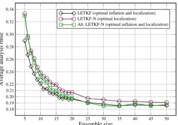
In Fig. 6 are plotted the best rmses for the three filters, with localization.
LETKF-N is always slightly suboptimal (with a maximal discrepancy of 10 % forN=5). However, it is the only un-conditionally stable filter of the three: it does not require in-flation.
The alternate LETKF-N is as good as LETKF-N for small ensembles but it does require inflation, which is why it is not so interesting in this regime. The alternate LETKF-N is as good as LETKF in thelarge ensemble size regime, but without inflation.
As we increase the time interval between updates, the performance of the filters degrades but their relative perfor-mance evolves. Let us take the example of an ensemble size of N=10, following Harlim and Hunt (2007). The setup is unchanged except for the time interval between updates which is set to1t=0.05,0.10,...,0.50. The results are re-ported in Fig. 7.
For1t≤0.20, LETKF with optimal inflation and localiza-tion outperforms LETKF-N with optimal localizalocaliza-tion and no inflation. For1t≥0.20, LETKF-N dominates. Like in the Lorenz ’63 case, this is reminiscent of the results of Harlim and Hunt (2007). This indicates that the relative performance of filters as shown for instance by Fig. 6 should not be taken as a rule, since there are regimes where LETKF-N (without inflation) performs better than LETKF.
The good performances of EnKF-Ns relative to the EnKFs in the strong nonlinear regime, is not an indication that EnKF-N can handle non-Gaussianity in this regime. How-ever the sampling errors may be created and exacerbated by the linearity of the model flow, and hence of the non-Gaussianity of the underlying pdf of errors. This may give an advantage to the finite-size ensemble filters in this regime.
6 Summary and future directions
Current strategies for stabilizing the ensemble Kalman fil-ter are empirical tuning of inflation, use of multi-ensemble configuration, explicit identification of the sampling/model errors, or adaptive optimization of inflation. In this article, we have followed a somehow different route. A new back-ground prior pdf that takes into account the discrete nature of the ensemble was derived using Bayesian principles. It accounts for the uncertainty attached to the first- and second-order empirical moments of the ensemble seen as a sample of a true error distribution. The definition of the prior pdf leads to a new class of filters (EnKF-N). Even though the re-sulting prior is non-Gaussian, it is entirely based on Gaussian hypotheses for the errors. In principle, through this prior, the analysis should take into account sampling errors.
Specifically, an ensemble transform variant (ETKF-N) was derived in the spirit of the ETKF of Hunt et al. (2007). It is tested on the Lorenz ’63 and the Lorenz ’95 toy models. In the absence of model error, the filter appear to be stable without inflation for ensemble size greater than the model unstable subspace dimension of the attractor. Moreover, for large enough time interval between updates, its performance is superior to that of ETKF. A variant of ETKF-N is expected to outperform ETKF-N for small time interval between up-dates: without inflation, it seems to systematically perform as well as, or better than ETKF. Unfortunately, as shown in the case of the Lorenz ’95 model, these finite-size filters diverge for smaller ensemble size, like any ensemble Kalman filter. Localization is mandatory. That is why a local variant of the filter (LETKF-N) which parallels LETKF, is developed.
From experiments on the Lorenz ’95 toy model, LETKF-N scheme seems stable without inflation. Depending on the time interval between updates, its performance with opti-mally tuned localization can be slightly inferior or superior to LETKF with optimally tuned localization and optimally tuned inflation.
The methodology presented here is mainly aproof of con-cept. We believe that more work is needed to explore the strengths and limitations of the methodology, and that there is room for improvement of the schemes.
For instance, we conjectured that the incapacity of ETKF-N to fully account for sampling errors (as opposed to LETKF-N with optimally tuned localization), was mainly due to the use of an hyperprior which generates correlations different from that of the data assimilation system built on the particular model. To avoid using weakly informative (hyper)priors onxbandB, one solution is to pass
5 6 7 8 9 10 11 12 13 14 15 16 17 18 19 20 25 30 35 40 45 50 1.0
1.0051.01 1.0151.02 1.0251.03 1.0351.04 1.0451.05 1.0551.06 1.0651.07 1.0751.08 1.0851.09 1.095
Inflation factor
(a) LETKF
5 6 7 8 9 10 11 12 13 14 15 16 17 18 19 20 25 30 35 40 45 50
Ensemble size
0.95 0.9550.96 0.9650.97 0.9750.98 0.9850.99 0.9951.0 1.0051.01 1.0151.02 1.0251.03 1.0351.04 1.0451.05 1.0551.06 1.0651.07 1.0751.08 1.0851.09 1.095
Inflation factor
(b) LETKF-N
5 6 7 8 9 10 11 12 13 14 15 16 17 18 19 20 25 30 35 40 45 50
Ensemble size
1.0 1.0051.01 1.0151.02 1.0251.03 1.0351.04 1.0451.05 1.0551.06 1.0651.07 1.0751.08 1.0851.09 1.095
Inflation factor
(c) Alt. LETKF-N
0.18 0.19 0.20 0.21 0.22 0.23 0.24 0.25 0.26 0.27 0.28 0.29 0.30 0.31 0.32 0.33 0.34 0.35 0.36
Fig. 5. Root mean square errors of LETKF(a), LETKF-N(b), and alternate LETKF-N(c), for a wide range of ensemble size (5–50) and inflation factorsr=1,1.005,...,1.095 and in panel(b)a larger range of inflation/deflationr=0.945,...,1.095.
The hyperprior forxbandBare chosen in such a way
(con-jugate distribution) that the posterior error covariance matrix still follows an inverse-Wishart distribution. However, such aBmatrix should be drawn from this distribution for each member, and the corresponding innovation statistics com-puted and inverted, which could become very costly. Even though one assumes all members use the same draw ofB, it is necessary to store the precision matrix9, which cannot be afforded in the high-dimensional context of geophysics. Still, to pass supplementary information (beyond the ensemble) one might contemplate adapting the algorithm of Myrseth and Omre (2010) so as to maintain a reduced-order, short memory, precision matrix, with a rank of a few ensemble sizes.
The behavior of EnKF-N in limiting regimes is worth ex-ploring. For instance, in the limiting case where the dy-namical model is linear, EnKF-N may not exhibit optimal
performance since EnKF-N does not make implicit assump-tions on the linearity of the model as opposed to traditional EnKFs. In this limiting case, the hyperpriorp(xb,B)should
optimally be a Dirac delta function pdf peaked at the empir-ical moments of the ensemble, which would make EnKF-N the traditional EnKF. But what happens to EnKF-N with Jef-freys’ hyperprior in this regime is less clear.
5 10 15 20 25 30 35 40 45 50
Ensemble size
0.18 0.19 0.20 0.21 0.22 0.24 0.26 0.28 0.30 0.32 0.34
Average analysis rmse
LETKF (optimal inflation and localization) LETKF-N (optimal localization)
Alt. LETKF-N (optimal inflation and localization)
Fig. 6. Best rmse over a wide range of inflation factors, and all possible localization lengths for LETKF and the alternate LETKF-N. Best rmse without inflation over all possible localization lengths for LETKF-N.
p(x|y,x1,...,xN)
= Z
dxbdBp(x|y,x1,...,xN,xb,B)p(xb,B|y,x1,...,xN) =
Z
dxbdBp(x|y,xb,B)p(xb,B|x1,...,xN) =p(y|x)
Z
dxbdB
p(x|xb,B)
p(y|xb,B)
p(xb,B|x1,...,xN). (52)
Because of the presence ofp(y|xb,B)in the last integral and
its dependence inxbandB, it seems difficult to analytically
solve the problem in order to generalize ETKF-N.
Stability without inflation is a property shared by ETKF-N, or LETKF-ETKF-N, with the multi-ensemble configuration of Mitchell and Houtekamer (2009). However the two ap-proaches draw their rationale from two different standpoints: Bayesian statistics and cross-validation respectively, whose connections are not clearly understood in Statistics. Addi-tionally, we note that the multi-ensemble approach makes use of the observation while the finite-size ensemble trans-form filters do not. In other words, the multi-ensemble ap-proach reduces the errors in the analysis while the finite-size ensemble transform filters do so prior to the analysis. The methodology developed in this article naturally led to deter-ministic filters, whose comparison with stochastic filters can-not be simple. Therefore it would be interesting to develop a stochastic filter counterpart to the deterministic EnKF-N presented here.
The focus of this study was primarily on sampling errors. In a realistic context, one should additionally take into ac-count model errors, and the errors that come from the de-viation from Gaussianity due to model non-linearity. If one
0.05 0.10 0.15 0.20 0.25 0.30 0.35 0.40 0.45 0.50
Time interval between updates ∆t
0.20 0.30 0.40 0.50 0.60 0.70 0.80
Average analysis rmse
LETKF (optimal inflation and localization) LETKF-N (optimal localization)
Fig. 7. Best rmse for LETKF and LETKF-N over all possible lo-calization lengths and a wide range of inflation factors for LETKF, for several time intervals between updates, and for an ensemble size
N=10.
trusts from the previous results that EnKF-N reduces signif-icantly the need for inflation meant to compensate for sam-pling errors, then the use of inflation in EnKF-N would es-sentially be a measure of model errors. It could also be a measure of the deviation from Gaussianity, or of the misspec-ification of the hyperprior as discussed earlier. These ideas have been successfully tested on the context of the Lorenz ’95 using the setup of this article. However, reporting these results is beyond the scope of this article.
As a final remark, we would like to mention that the prior pdfp(x|x1,...,xN)∝exp(−Jb(x)), whereJbis defined by
Eq. (21), could more generally be useful in environmental statistical studies, when one needs to derive a pdf from sam-ples of the system state, or of some error about it, which is assumed Gaussian-distributed. Note that the ensemble size needs to be large enough otherwise localization is still nec-essary.
Appendix A
One minimum or more
Here, the observation operator is supposed to be linear or linearized. Define the innovationδ=y−Hx. Equation (35) can be written
e
Ja(w)=1
2(δ−HXw)
TR−1(δ−HXw)
+N
2ln
1+ 1
N+w Tw
. (A1)
If there is a minimum, it must satisfy
"
(HX)TR−1HX+ N
1+N1+wTw
#
In order to diagonalize the left-hand side matrix, we can use the singular value decomposition
(HX)TR−1=UDVT, (A3) whereUis an orthogonal matrix inRN×N,Vis inRd×Nand
satisfies VTV=IN, and Dis a diagonal matrix in RN×N.
Definebw=UTw, then
"
D2+ N
1+N1+bwTbw
# b
w=Dv, (A4)
wherev=VTR−1/2δ. Then the left-hand side matrix is di-agonal.
In the case of a single observation (serial assimilation),D has only one non-zero entry (call itα), andDv is a vector with at most one non-zero entry (call itβ). Then solving for all the other components, it is clear that the components ofbw not related toαare zero. Then the remaining scalar equation for the non-trivial componentγ ofbwis
"
α2+ N
1+N1 +γ2
#
γ=β . (A5)
This third-order algebraic equation inγ has either one real solution or three real solutions. Therefore, the cost function
e
Ja has a global minimum, and possibly another local minimum. Note that with several observations assimilated in parallel, there may be more local minima.
Acknowledgements. The author acknowledges a useful discussion with C. Snyder on state-of-the-art ensemble Kalman filtering. The article has benefited from the useful comments and suggestions of L. Delle Monache, N. Bowler, P. Sakov acting as a Reviewer, an anonymous Reviewer, O. Talagrand acting as Editor, and L. Wu.
Edited by: O. Talagrand
Reviewed by: P. Sakov and another anonymous referee
References
Anderson, J. L.: An ensemble adjustment Kalman filter for data assimilation, Mon. Weather Rev., 129, 2884–2903, 2001. Anderson, J. L.: Exploring the need for localization in ensemble
data assimilation using a hierarchical ensemble filter, Physica D, 230, 99–111, 2007a.
Anderson, J. L.: An adaptive covariance inflation error correction algorithm for ensemble filters, Tellus A, 59, 210–224, 2007b. Anderson, J. L. and Anderson, S. L.: A Monte Carlo
Implementa-tion of the Nonlinear Filtering Problem to Produce Ensemble As-similations and Forecasts, Mon. Weather Rev., 127, 2741–2758, 1999.
Bishop, C. H. and Hodyss, D.: Flow-adaptive moderation of spu-rious ensemble correlations and its use in ensemble-based data assimilation, Q. J. Roy. Meteor. Soc., 133, 2029–2044, 2007. Bocquet, M., Pires, C. A., and Wu, L.: Beyond Gaussian statistical
modeling in geophysical data assimilation, Mon. Weather Rev., 138, 2997–3023, 2010.
Brankart, J.-M., Cosme, E., Testut, C.-E., Brasseur, P., and Ver-ron, J.: Efficient adaptive error parameterization for square root or ensemble Kalman filters: application to the control of ocean mesoscale signals, Mon. Weather Rev., 138, 932–950, 2010. Burgers, G., van Leeuwen, P. J., and Evensen, G.: Analysis scheme
in the ensemble Kalman filter, Mon. Weather Rev., 126, 1719– 1724, 1998.
Carrassi, A., Vannitsem, S., Zupanski, D., and Zupanski, M.: The maximum likelihood ensemble filter performances in chaotic systems, Tellus A, 61, 587–600, 2009.
Corazza, M., Kalnay, E., and Patil, D.: Use of the breeding tech-nique to estimate the shape of the analysis errors of the day, J. Geophys. Res., 10, 233–243, 2002.
Dee, D. P.: On-line Estimation of Error Covariance Parameters for Atmospheric Data Assimilation, Mon. Weather Rev., 123, 1128– 1145, 1995.
Desroziers, G., Berre, L., Chapnik, B., and Poli, P.: Diagnosis of observation, background and analysis-error statistics in observa-tion space, Q. J. Roy. Meteor. Soc., 131, 3385–3396, 2005. Evensen, G.: Sequential data assimilation with a nonlinear
quasi-geostrophic model using Monte Carlo methods to forecast error statistics, J. Geophys. Res., 99, 10143–10162, 1994.
Evensen, G.: Data Assimilation: The Ensemble Kalman Filter, Springer-Verlag, 2nd Edn., 2009.
Furrer, R. and Bengtsson, T.: Estimation of high-dimensional prior and posterior covariance matrices in Kalman filter variants, J. Multivariate Anal., 98, 227–255, 2007.
Gejadze, I. Y., Le Dimet, F.-X., and Shutyaev, V.: On analysis error covariances in variational data assimilation, SIAM J. Sci. Com-put., 30, 1847–1874, 2008.
Gottwald, G. A. and Mitchell, L., and Reich, S.: Controlling over-estimation of error covariance in ensemble Kalman filters with sparse observations: A variance-limiting Kalman filter, Mon. Weather Rev., 139, 2650–2667, 2011.
Hamill, T. M., Whitaker, J. S., and Snyder, C.: Distance-dependent filtering of background error covariance estimates in an ensemble Kalman filter, Mon. Weather Rev., 129, 2776–2790, 2001. Harlim, J. and Hunt, B.: A non-Gaussian ensemble filter for
as-similating infrequent noisy observations, Tellus A, 59, 225–237, 2007.
Houtekamer, P. L. and Mitchell, H. L.: Data assimilation using an ensemble Kalman filter technique, Mon. Weather Rev., 126, 796– 811, 1998.
Houtekamer, P. L. and Mitchell, H. L.: A sequential ensemble Kalman filter for atmospheric data assimilation, Mon. Weather Rev., 129, 123–137, 2001.
Huber, P. J.: Robust regression: Asymptotics, conjectures, and Monte Carlo, Ann. Statist., 1, 799–821, 1973.
Hunt, B. R., Kostelich, E. J., and Szunyogh, I.: Efficient data as-similation for spatiotemporal chaos: A local ensemble transform Kalman filter, Physica D, 230, 112–126, 2007.
Jeffreys, H.: Theory of Probability, Oxford University Press, 3rd Edn., 1961.
Lei, J., Bickel, P., and Snyder, C.: Comparison of Ensemble Kalman Filters under Non-Gaussianity, Mon. Weather Rev., 138, 1293– 1306, 2010.
Livings, D. M., Dance, S. L., and Nichols, N. K.: Unbiased ensem-ble square root filters, Physica D, 237, 1021–1028, 2008. Lorenz, E. N.: Deterministic nonperiodic flow, J. Atmos. Sci., 20,
130–141, 1963.
Lorenz, E. N. and Emmanuel, K. E.: Optimal sites for supplemen-tary weather observations: simulation with a small model, J. At-mos. Sci., 55, 399–414, 1998.
Mallat, S., Papanicolaou, G., and Zhang, Z.: Adaptive covariance estimation of locally stationary processes, Ann. Stat., 26, 1–47, 1998.
Mitchell, H. L. and Houtekamer, P. L.: An adaptive ensemble Kalman filter, Mon. Weather Rev., 128, 416–433, 1999. Mitchell, H. L. and Houtekamer, P. L.: Ensemble Kalman Filter
Configurations and Their Performance with the Logistic Map, Mon. Weather Rev., 137, 4325–4343, 2009.
Muirhead, R. J.: Aspect of Multivariate Statistical Theory, Wiley-Interscience, 1982.
Myrseth, I. and Omre, H.: Hierarchical Ensemble Kalman Filter, SPE J., 15, 569–580, 2010.
Ott, E., Hunt, B. R., Szunyogh, I., Zimin, A. V., Kostelich, E. J., Corazza, M., Kalnay, E., Patil, D. J., and Yorke, A.: A local ensemble Kalman filter for atmospheric data assimilation, Tellus A, 56, 415–428, 2004.
Raynaud, L., Berre, L., and Desroziers, G.: Objective filtering of ensemble-based background-error variances, Q. J. Roy. Meteor. Soc., 135, 1177–1199, 2009.
Sacher, W. and Bartello, P.: Sampling Errors in Ensemble Kalman Filtering. Part I: Theory, Mon. Weather Rev., 136, 3035–3049, 2008.
Sakov, P. and Bertino, L.: Relation between two common local-isation methods for the EnKF, Comput. Geosci., 15, 225–237, 2010.
Sakov, P. and Oke, P. R.: Implications of the Form of the Ensem-ble Transformation in the EnsemEnsem-ble Square Root Filters, Mon. Weather Rev., 136, 1042–1053, 2008.
Tippett, M. K., Anderson, J. L., Bishop, C. H., Hamill, T. M., and Whitaker, J. S.: Ensemble square root filters, Mon. Weather Rev., 131, 1485–1490, 2003.
van Leeuwen, P. J.: Comment on Data Assimilation Using an Ensemble Kalman Filter Technique, Mon. Weather Rev., 127, 1374–1377, 1999.
Wang, X., Bishop, C. H., and Julier, S. J.: Which is better, an en-semble of positive-negative pairs or a centered spherical simplex ensemble?, Mon. Weather Rev., 132, 1590–1605, 2004. Whitaker, J. S. and Hamill, T. M.: Ensemble Data Assimilation
without Perturbed Observations, Mon. Weather Rev., 130, 1913– 1924, 2002.
Wick, G. C.: The Evaluation of the Collision Matrix, Phys. Rev., 80, 268–272, 1950.
Zhou, Y., McLaughlin, A., and Entekhabi, D.: Assessing the per-formance of the ensemble kalman filter for land surface data as-similation, Mon. Weather Rev., 134, 2128–2142, 2006.