Level density for deformations of the Gaussian orthogonal ensemble

Level density for deformations of the Gaussian orthogonal ensemble

A. C. Bertuola, J. X. de Carvalho, M. S. Hussein, M. P. Pato, and A. J. Sargeant

Instituto de Física, Universidade de São Paulo, Caixa Postal 66318, 05315-970 São Paulo, São Paulo, Brazil sReceived 6 October 2004; published 17 March 2005d

Formulas are derived for the average level density of deformed, or transition, Gaussian orthogonal random matrix ensembles. After some general considerations about Gaussian ensembles, we derive formulas for the average level density for sid the transition from the Gaussian orthogonal ensemblesGOEd to the Poisson ensemble andsiidthe transition from the GOE tomGOEs.

DOI: 10.1103/PhysRevE.71.036117 PACS numberssd: 05.30.Ch, 05.45.Mt, 05.40.2a, 24.60.2k

I. INTRODUCTION

Deformed random matrix ensembles were introduced by Rosenzweig and Porterf1,2gto classify the conservation of electronic spin and orbital angular momentum in the spectra of complex atoms. Many varieties of deformed ensembles have since been constructed. Recent reviews of deformed ensemblessthey are also called transition ensemblesdcan be found in Refs.f3,4g. Earlier results on deformed ensembles were reviewed in Ref.f5g. Among the applications they have found, we mention the breaking of time-reversal invariance

f6gand the breaking of symmetriesf7g.

In this paper, we are concerned with the level density for deformed Gaussian orthogonal random matrix ensembles. Although the level density of the standard random matrix ensembles is not directly related to the physical many-particle level density, it is essential to the proper unfolding of fluctuation measures f8g. Unfolding is a transformation which leaves sequences of energy levels with a constant av-erage density. Normally, experimental energy levelsandthe

energy levels obtained from random matrix theory are un-foldedswhich removes the secular energy dependencesd be-fore fluctuation measures for both are calculated and com-pared. While the level densities of most random matrix ensembles are different, the bheavior of the fluctuation mea-sures of a wide class of ensembles is the same and hence denominated universal. For instance, each of the non-Gaussian ensembles studied in Ref.f9g is shown to have a characteristic average level density, however after unfolding, the nearest-neighbor spacing distributions and number vari-ances of all are found to be identical to those of the standard Gaussian random matrix ensemblesf10g.

In the following, we derive formulas for the level density of two deformations of the Gaussian orthogonal ensemble

sGOEd. The first describes a transition from the GOE to an ensemble with Poisson fluctuation statistics, that is, from the GOE to an ensemble of diagonal matrices whose elements are independently Gaussian distributedf11,12g. Such random matrix models are of interest to the analysis of experimental data f13g and of dynamical models f14g whose fluctuation properties are intermediate between Poisson and GOE. The second deformation describes the transition from the GOE to

mGOEs, that is, from the GOE to a block diagonal matrix

withmblocks each of which is a GOEf15–17g. If the blocks

are labeled by quantum numbers such as angular momentum

f1g or isospin f18g, then the transition ensemble classifies

their conservation or nonconservation. ThemGOE to GOE

transition is also relevant to the analysis of symmetry break-ing in quartz blocksf19–21g.

Our method extends that of Wignerf22g, who showed, by assuming that terms containing patterns of unlinked binary associations dominate the averages of the traces of powers of matrices, that the level density for certain random matrix ensembles could be simply expressed as a Fourier of trans-formssee also Sec. III D of Ref.f5gd. Previous results for the level density of deformed GOEs have been derived using Stieltjes transform methods f23,24g. These methods are in fact general enough to treat deformations of, and interpola-tions between, any class of matrix ensemble. However, the formulas obtained in the present paper have the advantage that they are explicit and simple to evaluate numerically. Other methods for calculating the level density f25,26g are restricted to deformations of the Gaussian unitary ensemble

sGUEd.

II. INTERPOLATING GAUSSIAN ENSEMBLES

The joint probability distribution of the matrix elements of a matrix,H, for an interpolating Gaussian ensemble may

be expressed as

PsH,A,Bd=Z−1sA,Bdexpf−sAtrH2+BtrH₁2dg, s1d

whereZ is a normalization factor and trHdenotes the trace

ofH. The structure of the matrixH₁is chosen in such a way

that it defines a subspace of H. The parameters A and B

define thesenergydscale and degree of deformation. When

B→0, the joint distribution becomes

PsH,A,0d=Z−1sA,0dexps−AtrH2d. s2d

If we assume thatHis real symmetric, then the variances are

given by

H_ij2=1 +dij

4A , s3d

so that the limit B→0 defines the GOE. WhenB→`, the

elements ofH₁ vanish andH is projected onto a sparse

ma-trix,H₀, whose elements are on the complementary subspace

ofH₁. Therefore, the random matrices generated by Eq.s1d

H=H₀+H₁, s4d

with the variances of the matrix elements ofH₀given by the

right-hand side of Eq.s3dand those ofH₁given by

H₁2_ij= 1 +dij

4sA+Bd. s5d

This shows that whenB goes from zero to infinity, the

en-semble undergoes a transition from GOE to the Gaussian ensemble of sparse matrices defined by the choice of the structure ofH₁or, equivalently, ofH₀. It is also instructive to

introduce the parameter

a=s1 +B/Ad−1/2, s6d

which measures the relative strength ofH₁andH₀. The

tran-sition froma=0 toa=1 corresponds to the transition from

B=` toB=0.

III. LEVEL DENSITY FOR THE GOE

We now proceed to give a derivation of the semicircle law, valid for the GOE, which is equivalent to Wigner’s for the ensemble of random sign symmetric matrices f22g. In general, the average level densitysALDdmay be written as a Fourier transform,

rsEd= 1 2p

E

₋`

`

dkFskde−ikE_{, s7d}

where

Fskd=

E

−`

`

dErsEdeikE _s8d

=

o

n=0

`

sikdn n!

E

_−`

`

dErsEdEn_{. s9d}

LetEkdenote the eigenvalues of an N3N matrixH, which

satisfies Eqs.s2dands3d. From the exact expression,

rsEd= 1

N

o

k=1

N

dsE−Ekd, s10d

for the ALD, one obtains the following connection between the moments of the eigenvalue distribution and the moments of the matrix elements,

En;

E

−` `

dErsEdEn= 1 NtrH

n_{. s11d}

Substituting Eq.s11dinto Eq.s9d, we obtain

Fskd= 1 N

o

_n=0

`

sikdn n! trH

n_{. s12d}

It is also useful to note that by differentiating Eq. s8d, the moments of the eigenvalue distribution can be expressed as derivatives of the Fourier transform of the ALD evaluated at zero, that is,

En=i−nFsnds0d, s13d

whereFsnd_s0d=fdn_F/dkn_gk

=0.

For large matrices,N@1, the average of the trace is domi-nated by the terms in which matrix indices may be con-tracted in such a way that we are left withs=n/2 pairs of

matrix elements. This means that we can write

trHn.CsNs+1s2s, s14d

where we have introduced the notation

s2= 1

4A s15d

for the variance of the off-diagonal matrix elements. The factor Cs counts the number of contractions that leads to

pairs. We observe that in a contraction, s−1 indices are

eliminated ands+1 remain, which explains the power ofN

in the above expression and allows us to write

Cs=

1

s

s2sd!

ss− 1d!ss+ 1d!, s16d

where the binomial factor counts the number of ways s+1

indices can be extracted out of 2s ones. The factor is then

divided bys, that is, the number of wayss−1 indices can be

eliminated without changing the contraction.

Substituting Eq.s14din Eq.s12d, we find that the Fourier transform of the average density is given by

F₁sa,kd . 1 ka/2

o

_s=0

`

s−ds_ska/2d2s+1

s!ss+ 1d! =

1

ka/2J1skad, s17d

whereJ₁sxdis a first-order Bessel function and

a=

Î

N/A. s18d

Using the formula

s1 −x2d1/2=1

2

E

_−`

`

y−1J₁syde−ixydy, s19d

the Fourier transform in Eq.s7dmay be evaluated to obtain the semicircle law,

r1sa,Ed=

5

1 pa2/2

Î

a

2_−E2_{, uEuøa,}

0, uEu.a,

s20d

where the radius of the semicircle is given by Eq.s18d. The cumulative level densitysCLDd,xsEd, is defined by

xsEd=

E

0

E

rsE

₈

ddE

₈

, s21d

x₁sa,Ed=

5

− 1/2, E,a,

E

Î

a2−E2+a2arcsinsE/ad

pa2 , uEuøa,

1/2, E.a.

s22d

The average number of levels up to energy E is given in

terms of the CLD byNfxsEd−xs−`dg.

IV. THE TRANSITION GOE TO POISSON

Before considering the transition from Poisson to GOE, we derive a formula for the ALD for a more general case.

A. Level density forH₀₊H₁

The trace of thenth power of Eq.s4dcan be written as

trHn= trsH₀+H₁dn=

o

l=0 n

n! l!sn−ld!trH0

l_H

1

n−l_.

s23d

IfH₀andH₁are statistically independent, we can write

trH₀lH₁n−l=

o

j

E₀j l _kjuH

1

n−l_{ujl s24d}

=E₀l trH₁n−l, s25d

where E_0j and ujl are defined by the eigenvalue equation H₀ujl=E₀jujl and E₀l denotes the lth moment of the

eigen-value distribution ofH0. Equationss23dands25dallow us to writefcf. Eq.s11dg

1

NtrH n_<

E

−` `

dE₀r₀sE₀d

E

−`

`

dE₁r₁sE₁dsE₀+E₁dn, s26d

wherer0 andr1are the average level densities correspond-ing toH₀andH₁, respectively. Equations26dis only

approxi-mate because in resumming the binomial series we have kept linked as well as unlinked binary associations ofH₀andH₁.

In the following subsection, we show that for the case of the transition GOE-Poisson the resulting discrepancy in the ALD is small. We also show how to correct for this discrepancy.

Substituting Eq.s26dinto Eq.s12d, we find

Fskd=

E

−` `

dE₀r0sE0d

E

−`

`

dE₁r1sE1deiksE0+E1d=F0skdF1skd,

s27d

where F₀ and F₁ are the Fourier transforms of r0 and r1, respectively. The ALD is obtained by substituting Eq. s27d

into Eq. s7d. Another representation is obtained by noting that since Eq. s27d is a product of Fourier transforms, the ALD ofHis given by the convolution of the average level

densities ofH₀andH₁,

rsEd=

E

−` `

dE

₈

r0sE

8

dr1sE−E

8

d. s28d

The only assumption required to derive Eqs.s27dands28dis that the matrix elements of H₀ andH₁ be statistically

inde-pendent.

B. Level density for the transition GOE to Poisson To specialize the results of the last subsection to the tran-sition GOE-Poisson,H₀ is chosen to be the diagonal matrix H₀ij=E0idijwhose eigenvalues, E0i, are independent random

variables with Gaussian distribution

r0sEd=

Î

A

pe

−AE2_{. s29d}

The variance ofH₀ is thus

H₀2_ij= dij

2A=a

2dij

2N. s30d

We choose H1 to be a diagonal-less matrix whose matrix elements are independent Gaussian variables with zero mean and variances

H₁2_ij=a21 −dij 4A =a

2_a21 −dij

4N . s31d

The ALD forH₀alone is given by Eq.s29dand the CLD,

Eq.s21d, by

x₀sEd=1

2erfs

Î

AEd. s32d The Fourier transform of Eq.s29dis

F0skd=e−k

2_/4A

. s33d

Note that for fixeda,A_→` asN<sub>→</sub>`, so that

r₀sEd_→

N→`

dsEd. s34d

The ALD forH₁ alone is given byr1saa,Ed, that is, by the semicircle law fsee Eq. s20dg with the radius modified

sa_→aadin accordance with Eq.s31dfor the variance ofH₁ fcf. Eq.s3dg. Its Fourier transform isF₁saa,kd fsee Eq.s17dg.

The ALD forH₁is given by the semicircle law in spite of the

missing diagonal because off-diagonal matrix elements dominatesfor Nlarge enoughd.

Using Eqs.s27dands7d, the ALD which interpolates be-tween the Gaussian and the semicircle asavaries between 0 and 1 is then found to be

rasEd=

1 2p

E

₋`

`

dkF₀skdF₁saa,kde−ikE s35d

=2 p

Î

A

l

E

₀

`

dx

xe

−x2/4l2_J

1sxdcos

Î

AxE

l , s36d where we have changed the integration variable to x=aka

and introduced the parameter

l=a

Î

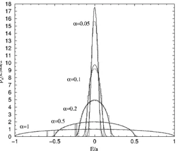
N. s37d

In Fig. 1, we compare Eq. s36d for rasEd with histograms

espe-cially apparent in the graph fora=0.05. The CLD, Eq.s21d, may be expressed using Eq.s36das

xasEd=

2 p

E

₀

`

dx x2e

−x2/4l2_J

1sxdsin

Î

AxE

l . s38d

This equation provides a more accurate manner of unfolding fluctuation measures than the polynomial unfolding used in Ref.f27g. Equations38dis plotted for several values ofain Fig. 2.

The ALD may be expressed alternatively using the con-volution formula, Eq. s28d. In particular, when N_→` for

fixedaanda, we find from Eq.s28dand Eq.s34dthat

rasEd→

N→`

r1saa,Ed. s39d

For finiteN, Eq.s28dyields

rasEd=

2

Î

N

p3/2a3a2

E

_−aa+E

aa+E

e−NE82/a2

Î

a2a2−sE−E

₈

d2dE. s40d

It it clear from these explicit formulas that the transition parameter isa2N, as was already argued in the original paper

of Rosenzweig and Porter f1g. The model described in this section can be cast in the form

H=H₀+ l

NcH1, s41d

withc=1/2, by modifying the definitions of the variances,

Eqs. s31d. Reference f26g considered the statistics of en-sembles of the form of Eq.s41dfor arbitraryc. In particular,

the asymptotic behavior of the ALD asN→`depends

criti-cally onc, Eq. s39dbeing valid only for the special case c

=1/2.

Equations36dmay be improved by comparing the result-ing lowest moments of the eigenvalue distribution with the average trace of the corresponding powers of the Hamil-tonian. Considering the latter first, we have

trH2= trH₀2+ trH2₁=NE₀2+C₁N2a

2_a2

4N = N

4Asl

2_{+ 2d}

s42d

and

trH4= trH₀4+ 4trH₀2H₁2+ trH₁4

=NE₀4+ 4E₀2C1N2 a2a2

4N +C2N

3a4a4 16N2

= N 8A2sl

4_{+ 4l}2_{+ 6d. s43d}

Inserting Eq. s36d into Eq. s13d for the moments of the ei-genvalue distribution, we find that

E2= 1

4A

₈

sl

8

2_{+ 2d, s44d}

E4= 1

8A

₈

2sl

8

4_{+ 6l}

8

2+ 6d. s45d

Note that the coefficient of l

8

2 in Eq. s45d is 6. This is a

result of the use of Eq. s26d, which included linked binary associations ofH₀andH₁. Equations11ddemands that

E2= 1 NtrH

2_{, s46d}

FIG. 1. Graph ofrasEd for several values ofa withN=1000.

The calculations were performed withA=N/4 for which the radius of the Wigner semicircle isa=2. The solid lines were calculated using Eq.s36dand the dotted histograms by numerically diagonal-izing an ensemble of 100 matrices.

FIG. 2. Graph ofxasEd calculated using Eq. s38d for several

E4= 1 NtrH

4_{. s47d}

Solving Eqs.s46d and s47d for A

₈

andl

₈

, we see that Eq.

s36dwill give the second and fourth moments of the eigen-values distribution correctly if we make the substitution

1

A→

1

A

₈

=

1

A

S

1 +l

2

F

_{1 −}

Î

_{1 +} 4

l2

G

D

, s48d

l2→l

8

2=l2

Î

1 + 4 l2

1 +l2

F

1 −

Î

1 + 4 l2

G

. s49d

In Fig. 3, we show the improvement to the ALD obtained by using Eqs.s48dands49din Eq.s36dfor the worst case of Fig. 1sa=0.05d. We see that the modified formula gives the ALD essentially exactly.

In Fig. 4, we show the peak value of the density of states as a function ofl ssee figure captiond. We see that both the modified and unmodified versions of Eq. s36d agree at the l=0 limit. We also see that both versions of Eq.s36dreach the N_→` limit fEq. s39dg at roughly the same value of lsl<6d. However, the two versions deviate from each other in the transition region, the largest difference occurring aroundl<1.5sa<0.05 forN=1000d. Also shown for

com-parison is the interpolation formula for the ALD of Persson and Åbergf28g,

r_aPA= N 1/2

4aN1/2+ 7N−1.5a. s50d

V. THE TRANSITION GOE TOm _GOES

We now calculate the ALD for the transition from the GOE to a superposition of m GOEs. To proceed, we again

consider an ensemble of matrices of the form of Eq. s4d. Now H₀ is a block diagonal matrix consisting of m blocks

whose dimensions are Mi, i=1,2,…,m, with oim=1Mi=N.

The elements ofH₀have zero mean and variances given by

Eq. s3d. We define H1 to be zero whereH0 is nonzero and elsewhere its elements have zero mean and variances given by Eq.s5d.

To obtain a formula for the ALD, we note that

trH2=

o

j,k=1

N

H2_jk s51d

=N2

o

i=1

m M_i

Nsi

2 _s52d

with

si

2₌ 1 4A

F

Mi

N +a

2

S

_{1 −}Mi

N

D

G

. s53d

Considering a single line ofH, thesi

2_{consist of a term which} is the product of the variance of a single nonzero element of

H₀with the probability for being in blockiplus a term which

is the product of the variance of a single nonzero element of

H₁with the probability for being outside blocki. In the sum

in Eq. s52d, the s_i2 are weighted with the fraction of lines which find themselves in blocki.

For the fourth power ofH, we find

trH4= 2

o

j,k,l=1

N

H2_jkH2_jl s54d

FIG. 3. Graph ofrasEd showing the improvement obtained by

demanding that the second and fourth moments of the eigenvalue distribution be exact fora=0.05 andN=1000. The solid lines result from using Eq.s36d and the dot-dashed lines from using the same equation modified in accordance with Eqs.s48dands49d. The dot-ted histograms were obtained by numerically diagonalizing an en-semble of 100 matrices.

FIG. 4. Graph of the peak values of the densityras0d, Eq.s36d,

as a function of the transition parameterl, Eq.s37d. For compari-son we also show the limiting casesr0s0d, Eq.s29d, andr1saa,0d, Eq.s39d, as well as an interpolation formula given by Persson and Åbergf28gr_aPA, Eq. s50d. Finally, we showras0dcalculated using

=2

o

j=1

N

F

o

k=1

N

H_jk2

G

2

s55d

=2N3

o

i=1 m

Mi

Nsi

4_{. s56d}

Although the authors were unable to obtain an equation analogous to Eq.s55dfor higher powers ofH, Eqs.s52dand s56dstrongly suggest that

trH2s_.C sNs+1

o

i=1

m M_i

Nsi

2s _s57d

for largeN.

Substituting Eq. s57dinto Eq. s12d and again using Eqs.

s17d,s7d, ands19d, we obtain

rsEd=

o

i=1 m

Mi

Nr1sai,Ed, s58d

wherer₁is given by Eq.s20dand

ai=a2

F

Mi

N +a

2

S

_{1 −}Mi

N

D

G

s59d

=1

A

F

Mi+l

2

S

_{1 −}Mi

N

D

G

. s60d

From Eq.s58d, it follows that the CLD, Eq.s21d, is given by

xsEd=

o

i=1 m

Mi

Nx1sai,Ed, s61d

withx₁ given by Eq.s22d.

In Fig. 5, we compare Eq.s58d. for the ALD with numeri-cal simulations for several values of theassee figure caption for detailsdand excellent agreement is obtained.

VI. CONCLUSION

In conclusion, by assuming that terms containing patterns of unlinked binary associations dominate the averages of the

traces of powers of matrices, we have derived formulas for the average level density for two deformations of the Gauss-ian orthogonal ensemble. The first describes the transition from the Gaussian orthogonal ensemble to the Poisson en-semble and the second the transition from the GOE to m

GOEs. The formulas obtained are in excellent agreemeent with numerical simulations.

ACKNOWLEDGMENTS

This work was carried out with support from FAPESP, the CNPq, and the Instituto de Milênio de Informação Quântica—MCT.

f1gN. Rosenzweig and C. E. Porter, Phys. Rev. 120, 1698s1960d, reprinted in Ref.f2g.

f2gC. E. Porter,Statistical Theory of Spectra: Fluctuationss Aca-demic, New York, 1965d.

f3gV. K. B. Kota, Phys. Rep. 347, 223s2001d.

f4gT. Guhr, A. Muller-Groeling, and H. A. Weidenmuller, Phys. Rep. 299, 189s1998d.

f5gJ. F. T. A. Brody, J. B. French, P. A. Mello, A. Pandey, and S. S. M. Wong, Rev. Mod. Phys. 53, 385s1981d.

f6gM. S. Hussein and M. P. Pato, Phys. Rev. Lett. 80, 1003 s1998d.

f7gM. S. Hussein and M. P. Pato, Phys. Rev. Lett. 84, 3783 s2000d.

f8gJ. B. French, V. K. B. Kota, A. Pandey, and S. Tomsovic, Ann.

Phys.sN.Y.d 181, 198s1988d.

f9gS. Ghosh, A. Pandey, S. Puri, and R. Saha, Phys. Rev. E 67, 025201sRd s2003d.

f10gO. Bohigas, inLes Houches LII: Chaos and Quantum Physics sElsevier, Amsterdam, 1991d, pp. 87–199.

f11gT. Guhr and H. A. Weidenmuller, Ann. Phys.sN.Y.d 193, 472 s1989d.

f12gM. P. Pato, C. A. Nunes, C. L. Lima, M. S. Hussein, and Y. Alhassid, Phys. Rev. C 49, 2919s1994d.

f13gA. Y. Abul-Magd and M. H. Simbel, J. Phys. G 24, 579 s1998d.

f14gM. Matsuo, T. Døssing, E. Vigezzi, and S. Åberg, Nucl. Phys. A 620, 296s1997d.

f15gT. Guhr and H. A. Weidenmuller, Ann. Phys.sN.Y.d 199, 412 FIG. 5. Graph of rasEd illustrating the transition 3 GOEs to

s1990d.

f16gM. S. Hussein and M. P. Pato, Phys. Rev. Lett. 70, 1089 s1993d.

f17gM. S. Hussein and M. P. Pato, Phys. Rev. C 47, 2401s1993d. f18gS. Åberg, A. Heine, G. E. Mitchell, and A. Richter, Phys. Lett.

B 598, 42s2004d.

f19gC. Ellegaard, T. Guhr, K. Lindemann, J. Nygård, and M. Ox-borrow, Phys. Rev. Lett. 77, 4918s1996d.

f20gA. Abd El-Hady, A. Y. Abul-Magd, and M. H. Simbel, J. Phys. A 35, 2361s2002d.

f21gK. Schaadt, A. P. B. Tufaile, and C. Ellegaard, Phys. Rev. E

67, 026213s2003d.

f22gE. P. Wigner, Ann. Math.62, 548s1955d, reprinted in Ref.f2g. f23gL. A. Pastur, Teor. Mat. Fiz. 10, 102 s1972d, fTheor. Math.

Phys. 10, 67s1972dg.

f24gA. Pandey, Ann. Phys.sN.Y.d 134, 110s1981d.

f25gT. Guhr and A. Müller-Groeling, J. Math. Phys. 38, 1870 s1997d.

f26gH. Kunz and B. Shapiro, Phys. Rev. E 58, 400s1998d. f27gA. J. Sargeant, M. S. Hussein, M. P. Pato, and M. Ueda, Phys.

Rev. C 61, 011302s2000d.