The non-linear evolution of magnetic flux ropes: 3. effects of dissipation

The non-linear evolution of magnetic flux ropes:

3. effects of dissipation

C. J. Farrugia1,2, V. A. Osherovich3, L. F. Burlaga4 1

Department of Mathematics, Science and Technical Education, University of Malta, Malta

2_{now at: Institute for the Study of Earth, Oceans and Space, University of New Hampshire, Durham, NH-03824, USA} 3

NASA-Goddard Space Flight Center, Hughes STX, Greenbelt, Md 20771 4

NASA-Goddard Space Flight Center, Code 692, Greenbelt, Md 20771

Received: 4 March 1996 / Revised: 2 September 1996 / Accepted: 4 September 1996

Abstract.We study the evolution (expansion or oscilla-tion) of cylindrically symmetric magnetic flux ropes when the energy dissipation is due to a drag force proportional to the product of the plasma density and the radial speed of expansion. The problem is reduced to a single, second-order, ordinary differential equation for a damped, non-linear oscillator. Motivated by recent work on the interplanetary medium and the solar corona, we consider polytropes whose index, c, may be less than unity. Numerical analysis shows that, in contrast to the small-amplitude case, large-amplitude oscillations are quasi-periodic with frequencies substan-tially higher than those of undamped oscillators. The asymptotic behaviour described by the momentum equation is determined by a balance between the drag force and the gradient of the gas pressure, leading to a velocity of expansion of the flux rope which may be expressed as…1=2c†r=t, whereris the radial coordinate and t is the time. In the absence of a drag force, we found in earlier work that the evolution depends both on the polytropic index and on a dimensionless parameter, j. Parameter j was found to have a critical value above which oscillations are impossible, and below which they can exist only for energies less than a certain energy threshold. In the presence of a drag force, the concept of a criticaljremains valid, and when j is above critical, the oscillatory mode disappears altogether. Furthermore, critical j remains dependent only on c and is, in particular, independent of the normalized drag coefficient, m3. Below critical j, how-ever, the energy required for the flux rope to escape to infinity depends not only on j (as in the conservative force case) but also on m3. This work indicates how under certain conditions a small change in the viscous drag coefficient or the initial energy may alter the evolution drastically. It is thus important to determine m3 andj from observations.

1 Introduction

In earlier work (Osherovichet al.1993a, 1995; hereafter referred to as Paper 1 and Paper 2, respectively) we studied the dynamics of self-similarly evolving cylin-drically symmetric magnetic flux ropes within the framework of ideal MHD. In Paper 1 we showed that a zero-beta flux rope can maintain self-similar oscilla-tions about the force-free state with a period which rises exponentially with the energy of the equivalent one-dimensional, non-linear oscillator. With a finite-beta plasma we found that the flux rope can not only oscillate but also expand to infinity (Paper 2). The general evolution can be classified in terms of two dimensionless parameters: the polytropic index, c, and a quantity j, the latter being a function of the plasma beta, the relative strength of the axial and azimuthal magnetic-field components of the flux rope, andc. The varieties of motion can be investigated for all subsets ofjÿcspace. Let us assume that initially the flux rope has a maximum of gas and axial-magnetic-field pressures on the symmetry axis, since this is the situation most favour-able for expansion (note that in Paper 2 we considered also flux ropes with a minimum of gas pressure on the symmetry axis). It was then found that, whereas for all j>1 and c>1 oscillation is the only mode of evolution, for c<1 and j>jcrit a critical value depending on c, expansion invariably results. For j<jcrit the mode of evolution depends on the energy of the oscillator. These results were obtained by the effective potential technique, which is possible since the system is conservative. The aim of this paper is to study flux-rope evolution when mechanical dissipation is present, and thus the approach of Papers 1 and 2 is no longer applicable.

The general motivation of this study is that the magnetic flux rope concept has proved useful in the modelling of various phenomena on the Sun, in the solar wind and in the geomagnetic tail (e.g. Stenflo, 1973; Osherovich et al.,1983; Elphic and Russell, 1983;

Moldwin, and Hughes, 1991; Sibecket al.,1984: see also the review by Gosling, 1990, and the book by Priest, 1982, and references therein). This theoretical and observational interest in the formation and evolution of magnetic flux ropes leads us to extend the rigorous MHD study of the evolutionary aspect, which naturally should include dissipation effects. As a first step, we study here dissipation due to a drag force.

There are at least two dissipative processes which one may wish to consider when treating this problem in a fluid approximation. The first is related to the finite electrical conductivity of the plasma. In this case, the induction equation of ideal MHD has to be modified to include a resistive term. The resulting loss of energy could be in the form of Joule heating of the plasma or reconnection processes. A second dissipative process is of a mechanical nature. The flux rope does not expand in a vacuum, and during its evolution it loses energy to its surroundings through viscous forces. To take account of this viscous drag, the momentum equation should be augmented by an extra term. While clearly both these dissipative mechanisms may influence the dynamics of magnetic flux ropes, we shall deal here only with the second mechanism.

In treating the resulting set of MHD equations, the approach of Papers 1 and 2 is no longer appropriate, and the concepts of effective potential, threshold energy as a potential barrier, etc. are no longer applicable. The concept of jcrit is still valid and, perhaps surprisingly, the value ofjcritdoes not depend on the drag coefficient, m3, which will be introduced. Thus, a categorization of phase orbits into open (expansion to 1) and closed (approach to an equilibrium position) is still possible. Forc>1 it is clear that, irrespective of the value ofm3, the only possible mode of evolution is still (damped) oscillation. Forc<1, whether oscillation or expansion takes place depends on the values of the parameters j;m3 and the initial energy. Parameter j is directly proportional to the plasma b, which appears as coefficient in the radially outward-pointing gas pressure term in the momentum equation. For givenc<1, and any finite m3, the condition j>jcrit is sufficient to ensure expansion to 1. On the other hand, for given values of the parameters c…<1†; j<jcrit and initial energy, one can always find a large enough drag coefficient such that the system is trapped and the motion is oscillatory. Thus the same regimes of evolution result as for m3ˆ0. Determining the initial energy as a function of c;j and m3 for the system to expand to infinity (‘escape energy’, Eesc) is a formidable task we do not attempt here. Instead, we shall limit ourselves to a comparison of the escape energy for select values ofjand m3 at fixedc…<1†with the correspond-ing values when m3ˆ0.

As in Paper 2 we shall consider polytropes with indices which may be larger or less than unity. Recent work on the interplanetary medium and the solar corona indicate that polytropes withc<1 do occur in practice and are important. Thus, the dynamics of that class of interplanetary ejecta called magnetic clouds (Burlagaet al., 1981) are found to be dominated by the

electron component which, further, is found to obey a polytropic relationship with a polytropic index,c_e0:5 (Osherovich et al.,1993b; Farrugia et al.,1994). In the solar context, a ‘velocity filtration’ mechanism has been put forward (Scudder, 1992a, b). With this mechanism the lower corona may be heated by utilizing the energy in the suprathermal tails of electron distributions at the base of the transition region without the need of further energy deposition. Non-Maxwellian distributions in a low-density plasma may lead to a value of c_e which is less than unity.

The layout of the paper is as follows. In the next section we separate the momentum equation and reduce the set of MHD equations to a single, non-linear, second-order, ordinary differential equation for the evolution function. In Sect. 3 we study analytically limiting cases of this equation. We linearize the evolution equation and discuss small-amplitude oscilla-tions about the stable equilibrium position. We focus on the dependence of the frequency on the drag coefficient and the plasma b. We then study the asymptotic behaviour of those flux ropes which expand to infinity and obtain an analytical expression for the velocity in the long time limit. The fourth section contains numerical studies of (a) non-linear, self-similarly ex-panding flux ropes, and (b) fully non-linear, finite-amplitude oscillations. For both cases we present exact numerical solutions and analyse the relative influence of the various forces on the course of evolution. By comparing the numerical with the analytical results, we can study the influence of the non-linearity on the dynamics of the magnetic flux ropes. Our solutions illustrate the sensitive dependence of the escape energy on the drag force. We also assess the errors introduced in an estimate of the ‘age’ of an expanding magnetic flux rope (i.e. the duration of self-similar expansion) when simple formulae strictly applicable only to the asympto-tic regime are used throughout.

2 MHD equations with drag force: derivations of the evolution equation

We employ the same set of MHD equations as inPaper 2 but add an extra term in the momentum equation. This drag force term is assumed proportional to the mass density of the plasma, q, and to the velocity, v, referred to the symmetry axis of the rope. The momentum equation is then (Gaussian units)

q@v=@t‡q…v1rv† ˆ1=4p…r2B2B†ÿrPÿmqv: …1†

In Eq. 1 B is the magnetic field, P is the gas pressure, vis the velocity and mis the drag coefficient. The other MHD equations are the divergence-free condition on B

r 1Bˆ0; …2†

the induction equation for an infinitely conducting fluid

@B=@tˆ r2 …v2B†; …3†

@q=@t‡ r 1 …qv† ˆ0; …4† and a polytropic equation of state

@=@t…P=qc† ‡ …v1r†…P=qc† ˆ0: …5† For self-similar magnetic fields (seePaper 1, 2) the two components of the magnetic field in cylindrical co-ordinates (r;/;z) can be expressed in the rest frame of the flux tube as

B…g;t† ˆB1…g†yÿ1…t†e/‡B0…g†yÿ2…t†ez; …6†

wheretis the time andgis the self-similarity parameter defined by

gr=y…t†: …7†

The function y…t†is the evolution function, which may be thought of as the radial scale of the magnetic flux tube. The dynamics of the configuration is determined by the functiony…t†.

In Papers 1 and 2we reduced the set of ideal MHD

equations to a single equation fory…t†by using separable magnetic fields, which are a sub-class of self-similar, cylindrically symmetric magnetic configurations. The introduction of a drag force makes the system non-conservative. However, even in the absence of a first integral of motion, one can still separate the momentum equation into a product of two functions, one depending only on t and other on g, and hence obtain a single differential equation fory…t†. The aim of the section is to present the derivation of this ‘evolution’ equation.

We restrict ourselves to radial flow, i.e

vˆv…r;t†er: …8†

The continuity Eq. 4 for the radially expanding flux rope is automatically satisfied if we introduce a stream functionDas follows:

qˆ ÿ…1=r† @D=@r …9a†

and

qvrˆ @D=@t: …9b†

If we now take the stream function, D, to be a single-parameter function (ofg), it can be shown from Eq. 9a, b that the density and radial velocity can be expressed as

qˆ ÿ…1=g†dD=dg yÿ2…t†; …10†

vˆ …r=y†dy=dt er: …11†

Collecting all velocity terms on the left-hand side of the momentum Eq. 1, we have

q‰@v=@t‡…v1rv†‡mvŠ ˆ1=4p…r2B2B† ÿ rP: …13† Using Eqs. 7, 9 and 11, the left-hand side of Eq. 13 can be written as

q‰@v=@t‡ …v1rv† ‡mvŠ ˆ ÿdD=dgyÿ2…t† ‰d2y=dt2 ÿmdy=dtŠ: …12† The polytropic relationship of Eq. 5 is satisfied by a gas pressure of the functional form

PˆP0…g†yÿ2c…t†: …13†

With Eq. 13, the right-hand side of Eq. 13 can be expressed as the sum of two terms, each a product of a function of gand a function oft, namely,

1=4p…r2B2B†ÿrPˆfÿ1=4pB0…g†dB0=dg‰yÿ5…t† ÿvyÿ3_{t†ŠÿdP0…g†=dgy}ÿ2cÿ1_t†g

er; …14† where the magnetic parameter v is defined by the following ratio

vˆ ÿ‰…B1=g†d=dg…gB1†Š = ‰B0dB0=dgŠ: …15†

As inPapers 1and2, we introduce next three constants, S, Q and K by

Sˆ …1=8p†d=dg…B20† =dD=dg; …16†

QˆSv: …17†

and

Kˆ ‰dP0=dgŠ = ‰dD=dgŠ: …18† Equating the right-hand sides of Eqs. 12 and 14, and using Eqs. 15–18, we reduce the momentum equation to a single equation for the evolution function, y…t† :

d2y=dt2ˆSyÿ3ÿQyÿ1‡Ky…ÿ2c‡1†ÿmdy=dt: …19† The evolution equation is thus a second-order, non-linear, ordinary differential equation with a dissipative term proportional to the first derivative of the evolution function. The left-hand side represents the inertial term. The magnetic forces are given by the first two terms on the right-hand side: the gradient of the axial-magnetic-field pressure …Syÿ3†and the pinch force …ÿQyÿ1†:The gas-pressure gradient term ‰Ky…ÿ2c‡1†] depends on the polytropic index,c, and the viscous drag term…ÿmdy=dt†

is proportional to the drag coefficient, m. For a maximum of the axial magnetic field pressure on the symmetry axis – the case we consider in this paper – parametersS andQare both>0:In addition, since we only study the case where the gas pressure maximizes on the axis of symmetry, we have K >0.

We shall work henceforth with the normalized form of Eq. 19. Instead ofyandt, we introduce a normalized evolution function and a normalized time by

Yˆy=y0 …20†

and

sˆtx0=p2; …21†

where y0 and t0 are defined, respectively, by

y0ˆS=Qvÿ1=2 …22†

and

x0ˆQ…2=S†1=2: …23† The frequencyxo defined here is the frequency of small oscillations of a zero-beta flux rope about its position of equilibrium, y0 (Paper 1). In Paper 2 we introduced further a normalizedK coefficient (j) by the formula

Introducing, finally, the normalized drag coefficient m3 by the substitution

m3ˆm…S1=2=Q†; …25† we can express the evolution equation, Eq. 19 in the normalized form (0ˆd=ds)

Y00ˆYÿ3ÿYÿ1‡jY…ÿ2c‡1†ÿm3Y0: …26† The physical meaning of the parametersy0,x0,jandm3 may be illustrated by considering their value for a magnetic flux rope of constant magnetic-field twist (‘Gold-Hoyle’ tube). Let us define the boundary of such a flux tube as the radial distance from the magnetic axis at which the axial field component,Bz, drops to one-fifth of its value on the magnetic axis, Bzmax. Further, let

B/max be the value reached by the azimuthal field component at this time. Assuming zero beta, the equilibrium position is then given by

y0ˆR0=4…B/max=Bzmax†2; …27†

and the corresponding period of oscillation,T0, by T0ˆ2p=x0ˆ …pR0=8vAz†…Bzmax=B/max†; …28† wheremAzis the Alfven speed, Bzmax=p4pqmax, andqmaxis the mass density on the magnetic axis (Paper 2). The parametersj andm3 can be expressed as

jˆ2…2cÿ4†b…Bzmax=B/max†…ÿ2c‡4† …29†

and

m3m…T0=21=2p†ˆ…m=27=2†…R=vAz†…Bzmax=B/max†: …30†

(Note that if another definition for the boundary of the flux rope is adopted, there will be some additional coefficients in Eqs. 29 and 30.)

Concerning the physical meaning of the parameters in the evolution equation, Eq. 26, we note first thatjis directly proportional to the plasma beta, but is also a function of the field ‘twistedness’ of the rope, and the polytropic index. Further, all the constants we have introduced in our illustration, namely, yo;T0;j and m3, are expressible in terms of measureable quantities, at least in principle. In particular, if the drag coefficient is known, then so ism3. Whilst the normalized coefficients have been derived above for a specific magnetic field (Gold-Hoyle), analogous formulae can be readily obtained for any separable magnetic field.

3 Analytically Tractable Cases

3.1 Small-amplitude oscillations with damping

We showed inPaper 2that for certain values ofjandc there exists a position of stable equilibrium (atYeq) such that

Y_eqÿ3ÿYÿ_eq1‡jY_eq…ÿ2c‡1†ˆ0: …31† Linearizing Eq. 26 about Yeq, we find that small-amplitude oscillations obey

DY00ˆ ÿx2_eqDYÿm3DY0; …32† where DY ˆY ÿYeq, with jDY=Yj 1, and x2eq is the solutions of

x2_eqˆ3Yÿ_eq4ÿY_eqÿ2ÿj…ÿ2c‡1†Yÿ2c

eq : …33†

In the absence of drag, Eq. 31 solved simultaneously with Eq. 33 allows us to recover the dependence of the frequency of small-amplitude oscillations on parameter j. According to Eq. 32, damping shifts all frequencies downwards to x, where

x2ˆx2_eqÿm32=4: …34† The damped, small-amplitude oscillations are given by

DYˆa eÿ…m3=2†scos…xs‡/† …35† where aand/are integration constants.

One can obtain the simultaneous solutions of Eqs. 31 and 33 in closed analytical form in certain special cases, namely, when cˆ1;3=2 and 2. The corresponding formulae are

x2_eqˆ2…1ÿj†2 …36† …cˆ1†,

x2_eqˆ3Gÿ4ÿGÿ2‡2jGÿ3 …37† fGj=2‡p…j2_=4‡1†g;

…cˆ1:5† and

x2_eqˆ2=…1‡j† …38† …cˆ2†.

In general, to express xeq as a function of j, we can proceed as follows. Combining Eqs.31 and 33 we can expressYeq in terms ofx2eq and c.

Yÿ_eq2 ˆ …1ÿc†=…4ÿ2c† ‡ f‰…1ÿc†=…4ÿ2c†Š2

‡x2eq=…4ÿ2c†g1=2: …39† We also have from Eq. 31

jˆ ‰1ÿYÿ_eq2Š=…Y_eqÿ2†…cÿ1†: …40† Substitution of Eq. 39 into Eq. 40 yieldsjas a function of x2

eq.

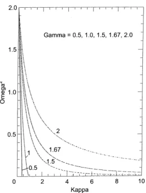
This relationship is inverted numerically and shown in Fig. 1, which plotsx2

oscillations are possible above a critical value of j (Paper 2). Both the drag force and the finite value ofb

decrease the frequency of small-amplitude oscillations (see Eq. 34 and Fig. 1). For finite-amplitude oscillations the frequency is further affected by the non-linearity of the system. We study this third source of frequency shifts in Sect.4.

3.2 Asymptotic behaviour of a self-similarly expanding magnetic flux rope

For a subset of values ofcandj, Eq. 26 has expanding solutions, i.e.Y increases monotonically to infinity with time. In these asymptotic solutions of Eq. 26 we assume that as s! 1, all forces become negligible except for the drag force and the gradient of gas pressure. Balancing these last two forces leads to the desired asymptotic behaviour. We finally check that the neglected terms were indeed negligible. Under these assumptions, ass! 1Eq. 26 reduces to the first-order equation

jY…ÿ2c‡1†ÿm3Y0ˆ0; …41† which integrates to

Yˆ …2cj=m3†1=2c s1=2c: …42† Substituting the asymptotic solution Eq. 42 in the full equation, Eq. 26, we find that the inertial term s…0:5=cÿ2† _{and the two magnetic terms …Y}ÿ3 _andYÿ1_† vary as sÿ2c _{and s}ÿ6c_{, respectively. For c<1}

(a necessary condition for expanding solutions) all these

three terms decrease in time faster than the drag force and gas pressure terms, each of which scales ass…0:5=cÿ1†_. Equation 42 is thus a valid asymptotic solution of Eq. 26 and for large times the evolution function has a power-law dependence on time. The slowest growth corre-sponds tocˆ1.

The resulting asymptotic velocity of the flux tube, i.e. Eq. 11, is

vˆ …r=y†dy=dterˆ …1=2c†…r=t†er: …43† The specific choice cˆ0:5 gives vˆr=t, which is the velocity of free expansion (Farrugia et al., 1993). For this case, the speed of the one-dimensional mechanical analogue (Y0) approaches a terminal value ofj=m3. For other values of c;Y0, and hence also the drag vary as …1=2c†…2cj=m3†1=2c s…1=2cÿ1†_{. In other words, the drag} force and the gas pressure term follow asymptotically the same power law. Furthermore, we note that the asymptotic velocity profile depends on the polytropic index and hence contains information on the thermo-dynamics of the expanding magnetic flux rope.

4 The full non-linear problem: numerical study

4.1 Expansion

We study first expanding solutions of Eq. 26. Following a discussion of the influence of the various forces in Eq. 26 on the history of the expansion, we present an explicit MHD solution. Finally, we estimate the duration of self-similar expansion from the asymptotic formulae derived in Sect. 3 and compare it to the value obtained from an exact solution.

The presence of the drag force requires us to integrate Eq. 26 numerically. To do this we first express Eq. 26 as a pair of coupled first-order differential equations

XˆY0; …44a†

X0ˆYÿ3ÿYÿ1‡jY…ÿ2c‡1†ÿm3X: …44b† As one of the initial conditions we choose X…0† ˆ0. Since we often compare results with those obtained for m3ˆ0, we find it useful to specifiyY…0†in the following way. We think of the corresponding problem with m3ˆ0 where the effective potential Ueff…Y† exists. We choose the initial energy, E…0†, to be a multiple of the minimum value of this Ueff, and then, solving the algebraic equation Ueff…Y† ˆE…0†; we obtain Y…0†, (where Ueff has no minimum, we use the minimum of

Ueff form3ˆbˆ0†:

The forces on the right-hand side of the evolution equation Eq. 26 are plotted on a log-log scale in Fig. 2. The parameters for this and all other illustrations in this sub-section are: cˆ2=3;jˆ1=2 and m3ˆ1=5. The initial energy is chosen to be 1, which is twice the minimum of Ueff for the zero-beta flux rope in the absence of the drag force. All force terms except the drag force are expressed as different powers of Y and hence they appear as straight lines on the log-log plot. To be noted is also that the variation of the drag force Fig. 1. The square of the frequency of small-amplitude, undamped

oscillations plotted as a function of parameter j for different polytropes (cˆ1₌2_;1_;3₌2_;5₌3_;2). All frequencies are below xˆ

with Y simultaneously illustrates the variation of speed of the equiavalent one-dimensional system,Y0. While the figure refers to the specific parameter set chosen, we find that the results themselves are representative of many parameter sets we tried.

Initially, the motion is dominated by the short-range term associated with the gradient of the axial magnetic pressure, B_z2, shown by curve A. This force leads to a rapid rise in the radial velocity away from the axis. Simultaneously, the drag force term (curve D) rises proportionately, slowing down the acceleration. At

Y ˆ1, the pinch term (curve C) balances the axial magnetic pressure term, which thereafter decreases very rapidly and plays no further role in the dynamics.

The system reaches maximum velocity shortly after

Y ˆ1 (i.e. at logY ˆ0†and then decelerates, mainly as a result of the pinch force. When the gas pressure term (curve B) overtakes the decreasing pinch force term, the speed …Y0† starts to decrease less steeply, i.e. it passes through a point of inflection in the vicinity of log

Y ˆ0:5. Y0 is almost constant for some time, during which the gas pressure term is pushing the system outwards. The drag force term approaches asymptoti-cally the falling (asYÿ1=3_{) gas pressure term. By this time} …logY >1:5† the pinch term has become negligible. Since the difference between the gradient of gas pressure and viscous drag terms approaches zero, the inertial term Y00 becomes negligible in comparison with these two forces.

Our numerical solution confirms the analytical results obtained in the previous section. Indeed, for large Y, the magnetic forces and the inertial term are negligible during the expansion and the dynamics are governed by the gradient of the gas pressure term and the drag force, which balance each other asymptotically. The normalized solution of the MHD equations for the choice of parameters in Fig. 2 is shown in the four panels of Fig. 3. From top to bottom, the first two panels show the evolution function Y…s† and its time

derivative,Y0…s†(which is equal to the radial velocity of the flux rope divided by the self-similarity parameter,g), respectively. The third panel shows the variation of the normalized gas pressure (continuous line) and density (dashed line) on the magnetic axis. The bottom panel shows the variation of the normalized magnetic field, also on the magnetic axis.

The density, gas pressure and axial field component are normalized using Eqs. 10, 13 and 6, respectively, and the definition of the normalized evolution function, Eq. 20. From these and Eq. 11 for the velocity we obtain the following expressions

vˆgY0…s†; …45†

qˆ ‰ÿ…1=g†dD=dgy_oÿ2ŠYÿ2…s†; …46† Pˆ ‰P0…g†yÿ₀2ŠYÿ2c…s†; …47† Bzˆ ‰B0…g†yÿ02ŠYÿ

2

s†: …48†

The ordinates in Fig. 3 representY;Y0…t†;Yÿ2…s†Yÿ2c…s†

Yÿ2_{s† as normalized values for the corresponding} physical quantities.

The evolution function in panel 1 shows a monotonic increase since the magnetic tube is expanding. The gas pressure, density and axial field all decrease in time as Fig. 2. The forces acting on an expanding flux rope plotted as

function ofY on a log-log scale. The parameters chosen arejˆ1=2;

cˆ2=3;m3ˆ1=5 andEˆ1:For further details, see text

negative powers of Y. In contrast, the speed of the equivalent one-dimensional system, Y0, is not a mono-tonic function of s, as already discussed in connection with the variation of the drag force in Fig. 2. Whereas, as shown in Sect. 2, the density and the axial field vary as the inverse square of Y, the gas pressure varies as

Yÿ2c_{; a consequence of the polytropic relationship;}

hence the crossover atY ˆ1 in the last-but-one panel. Figure 3 displays the temporal variation of the physical quantities. Stipulating a generating function satisfying certain physical conditions, self-similar dis-tributions D…g†;B0…g†;P0…g† and B1…g†, can be calcu-lated (see Papers 1 and 2). Equations 45–48 and Eq. 6 then allow us to recover the spatial and temporal variation of all relevant physical quantities (cf. the example of the Gold-Hoyle tube discussed in Paper 2).

We finally consider the determination of the duration of self-similar expansion, what we shall call the ‘age’ of the tube. Using the exact solution of Eq. 26, this age may be equated to the time, T, which it takes for the configuration to reach a givenY…T†. Instead of using the exact solution, we may alternatively use the simpler asymptotic formula Eq. 42. How does the last estimate compare with the exact age obtained numerically?

The bottom panel of Fig. 4 shows Y…s† calculated numerically (connected curve) andY…s†computed from Eq. 42 (dashed curve). The upper panel shows the

difference between these two estimates of age, expressed as a percentage of the exact age, as a function ofs. The 10% discrepancy level is indicated by the horizontal dotted line. It is clear that for a given size the asymptotic formula always underestimates the age of the flux rope. Initially, the discrepancy between the estimated ages is large (of order 40%). However, this difference decreases steadily, so that in the asymptotic region (forY >300) it has dropped to below 10%.

4.2 Oscillation

We now turn to finite-amplitude oscillations described by the evolution equation Eq. 26. In this sub-section we first present an analysis of the forces which govern the oscillatory motion. We then give an explicit numerical solution. We compare the exact results on finite-amplitude oscillations with the analytical formulas for small-amplitude oscillations discussed in Sect. 2 to illustrate the role of non-linearity in the flux rope’s behaviour, particularly as regards the frequency of oscillations. Finally, we discuss the dependence of the escape energy on plasma parameters, particularly the drag coefficient. We show how sensitive the system is to even a small variation inm3.

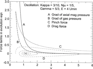
We consider first adiabatic…cˆ5=3†oscillations of a magnetic flux rope confining a plasma ofjˆ0:3 and a drag coefficientm3ˆ0:2. The energy of the oscillator is set initially at four times the minimum energy of the corresponding undamped oscillator, as explained earlier. Figure 5 plots the variation with Y of the four force terms on the right-hand side of Eq. 26. It may be considered as the counterpart of Fig. 2, but for oscillations. Note that both scales in Fig. 5 are linear. The history of the oscillatory motion can be described as follows: as for expansion, the system, is initially given a large outward acceleration by the gradient of the axial magnetic pressure (curve A). As a result of this, the

Fig. 4. The bottom panel shows a comparison of the exact numerical solutionY…s† (solid line) versus the analytical asymptotic solution (dot-dash line). Thetop panelplots the percentage age difference as a function ofsfor the same flux rope as in Figs. 2 and 3. Thedotted line indicates the 10% difference level

Fig. 5. The forces acting on an expanding flux rope as functions of

Y; plotted on a linear scale. The parameters chosen arejˆ3=10;

velocity, Y0, and hence the drag force (curve D) also increase. With increasing size of the tube (increase inY) the pinch (curve C) balances the magnetic-pressure gradient and a deceleration sets in. The gas-pressure gradient (curve B) contributes appreciably to the outward acceleration up toY 1. However, for Y >2 both gas pressure and magnetic pressure terms are negligible. Further dynamics are governed by the drag force opposing the pinch, leading to an almost constant deceleration of the system. Eventually the pinch reverses the motion. Thus the radial motion is initiated predominantly by the magnetic-pressure component of thejxBforce and is reversed by the tension component of the same force.

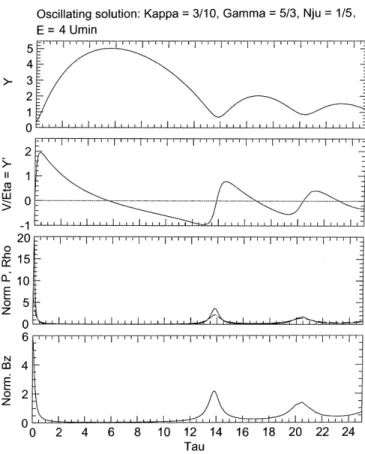
Figure 6 gives an explicit oscillating solution, calculated as for the expanding solution of Fig. 3, and shown in the same format as that figure. The same parameter set as for Fig. 5 is used. The upper panel shows the progressive decrease in both amplitude and period of the damped oscillations. The corresponding saw-tooth profile of the velocity, Y0, is shown in the second panel. As a result of the drag, the starting point of each successive swing advances inY (see upper panel or, better still, the curve D in Fig. 5). Thus the ‘kick’ given by the gradient of the axial magnetic pressure becomes progressively weaker. The resulting starting acceleration becomes correspondingly weaker with each swing, as can be seen in panel 2. The third and fourth panels show that the temporal variation of the pressure,

density and the magnetic field on the symmetry axis of the tube has an impulsive appearance of quasi-periodic character, with the amplitude of the disturbances decreasing rapidly with time. Because the period is getting steadily shorter, the relative drop in the amplitude is decreasing. At the same time, the pulses are becoming broader.

In the linear theory of Sect. 2 we discussed two reasons for the downward shift in frequency: the drag force and the presence of the plasma (finite-beta effects). Here we shall discuss the role that the non-linearity plays in determining the frequency of the oscillator. As our first illustration we consider the effect of finite beta on large-amplitude, damped oscillations.

We consider two magnetic flux ropes whose initial energy is the same and chosen to be four times the minimum of the effective potential whenbˆm3 ˆ0. The first has negligible gas pressure …bˆ0†and oscillates in a medium of drag coefficient = 0.2. The second differs from the first only in that it has a finite-beta plasma …bˆ0:8†. Figure 7 shows the result of this study. The dotted curves refer to the motion of the zero-beta tube, while the continuous curves refer to the finite-beta tube. The phase orbits of the equivalent non-linear oscillators plotted in the first panel both spiral towards their respective attractors after executing a number of

Fig. 6. Numerical solution for large-amplitude oscillations presented in the same format as Fig. 3 but with parameters as in Fig. 5

damped oscillations. The two positions of stable equilibrium are shifted in Y with respect to each other, each one corresponding to the minimum of Ueff when the viscous drag is absent. The decrease in amplitude,Y, due to damping is shown in the third panel, while the time variation of the corresponding velocities …Y0† for both oscillators is displayed in the middle panel. In both cases, the motion is damped and quasi-periodic. The frequency of oscillations for both increases steadily in time. Comparing frequencies, we find that the finite-beta tube has smaller frequencies than its zero-beta counter-part. Thus finite-beta effects act to lower the frequency, just as in linear theory.

The influence of gas pressure on the oscillations is also evident in the variation ofY0withs(middle panel). Two effects are present; (i) at the start of each oscillation, the amplitude ofY0 and the steepness of its rise is larger for the zero-beta tube; (ii) during the falling part of the oscillation, however, the speed of the finite-beta tube exceeds that of the zero-finite-beta tube. Since we chose the same initial energy for both oscillators, the initial value of Y for the zero-beta tube has a smaller value than for the finite-beta tube (see top panel). Consequently, the initial ‘kick’ (see above) due to the axial magnetic pressure term (Yÿ3† is larger for the zero-beta case. This explains (i). As we noted when examining the effect of the various forces on the oscillatory motion, in the case of finite beta the gas pressure provides an extra outward accelerating term; this explains (ii).

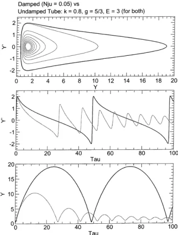
We next compare large-amplitude oscillations for two flux ropes with and without drag. The common parameters of the problem are cˆ5=3;jˆ0:8; initial energy = 3Ueff;min and for one flux tube m3 ˆ0:05: Figure 8 in the same format as Fig. 7 shows the results with dissipation (dotted lines) superimposed on those without dissipation (heavy lines). The latter show a closed phase orbit (first panel), and strictly periodic oscillation of Y and Y0 in the two other panels. By contrast, for the damped oscillations the first panel shows the phase orbit spiralling to the equilibrium position, while the other two panels display the damped quasi-periodic oscillations with frequencies which are throughout substantially higher than in them3ˆ0 case. Even though initially, Y…0† and Y0…0† are the same for both oscillators (top panel), the amplitudes for the dissipative case are from the start much lower and continue decreasing with time. Figure 8 illustrates the effect of the drag force on the frequency of large-amplitude oscillations. In Sect. 3 we found that the drag force decreases the frequency of small-amplitude oscilla-tions. Here we see that in the non-linear regime this effect is reversed.

To examine the linear regime numerically, we have to choose a value of the initial energy that is close to

Ueff;min: An example of such a calculation is shown in Fig. 9. We compare a damped …m3ˆ0:1† with an undamped oscillator…m3ˆ0†:The parameters common to both are the initial energy Eˆ1:01 Ueff;min; jˆ0:8; cˆ5=3: Even though the amplitude of the damped oscillator (dotted line in Fig. 9) steadily

decreases, the period remains unchanged from one oscillation to the next. Furthermore, this period is the same as that of the undamped oscillator (6.95 time units). The constancy of the period of the damped oscillator confirms that we are indeed in the linear regime. The lowering of the frequency due to damping expected from Eq. 34 is not evident in this instance, because this effect depends on the frequency ratiom32

4 x 2 eq: In our case, m32

4 ˆ2:5210ÿ 3_x2

eq1: To obtain a measurable effect we have to raisem3(we chosem3 ˆ0:6) keeping all other parameters the same. In Fig. 10 we plot the result in the same format as Fig. 9 where, however, because of the heavy damping we only show one cycle, marked by solid squares. There is an appreciable increase in period with respect to the undamped cycle (open squares; 7.35 vs 6.95 units). This example establishes consistency between our numerical scheme and the analytical results for the linear regime obtained in Sect. 3.

In Paper 2, which focused on conservative systems,

we found that for c<1 two modes of evolution are possible depending on the values of the energy, E; and the parameter j:We found that there is a critical value of j…jcrit†;which depends on c;above which expansion always occurs irrespective of the energy (see Eq. 30, Fig. 8. A comparison of large-amplitude oscillations of two flux tubes, one with damping (dotted lines) and one without (solid lines). The common parameters arejˆ0:8;cˆ5=3 andEˆ3:The panels show fromtop to bottomthe two phase orbits, and the variation ofY

Paper 2). For j<jcrit; however, there is a threshold energy to be overcome before the system can expand; otherwise, it just oscillates. In the low-j situation the effective potential has both a local minimum and a local maximum, and this threshold energy is equal to the local maximum of the effective potential.

The situation for the dissipative system is more complicated. The concept of jcrit and its related phase transition remain valid, but that of threshold energy requires modifications. As to the latter, we shall consider the amount of energy needed for the system to just manage to expand to infinity (‘escape energy’). The escape energy…Eesc†is a function not only ofjandcbut also ofm3:We now illustrate these two points in reverse order.

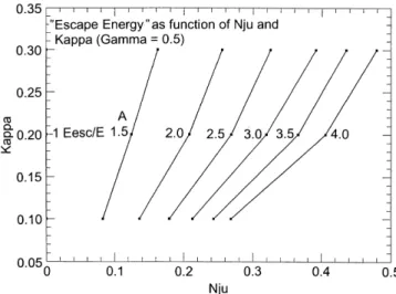
In Fig. 11, we study the dependence of Eesc on parameters jand m3 for a fixed value ofc…ˆ0:5†:We choose our values ofjto be below thejcritof the system whosem3 ˆ0:The points indicateEescfor a givenjand m3;andEescis measured in units of the threshold energy of the corresponding undamped case (i.e. same j but m3ˆ0) and shown by the row of numbers in the centre. Pairs of computed points …m3;j† for which Eesc is the same are joined by straight lines (note that the first line, for Eesc=Eˆ1; computed for them3ˆ0 case, coincides with the ordinate). The interpretation is straightforward.

For a given value ofEesc, one can find different pairs of …m3;j†such that the system with this initial energy will just be able expand to infinity. For example, for

Eescˆ3E; the system will just reach infinity if Fig. 9. A comparison of the small-amplitude oscillations of two flux

tubes, one with damping (dotted lines) and one without (solid lines) in the same format as Fig. 8. The damping coefficientm3 is = 0.1. The common parameters arejˆ0:8;cˆ5=3 andEˆ1:01

Fig. 10. Similar to Fig. 9 but this time with a much higher damping coefficient …m3ˆ0:6† in the same format as Fig. 8. The respective durations of one cycle can be read off from the marked positions of two successive maxima in thebottom panel

jˆ0:100 andm3ˆ0:213; jˆ0:200 andm3ˆ0:319;or jˆ0:300 andm3 ˆ0:391:The lines joining the points all have positive slope. This means that we can always offset an increase in the drag force by a simultaneous rise in the gas pressure. For fixed j; an increase in drag coefficient m3 requires a corresponding increase in the

Eesc (jump from line to line).

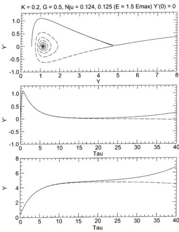
Figure 12 illustrates the sensitivity of the system to a change in m3: We choose the parameters corresponding to point A in the previous figure, i.e. jˆ0:2;

Eescˆ1:5E; m3ˆ0:124 and cˆ0:5: The open orbit shown by the solid curve in the three panels indicates that the flux rope can just expand to infinity after going through a stage of velocities0 (middle panel). If them3 coefficient is just raised by 10ÿ3 _{to 0.125, however, the} system is trapped, as shown by the dashed, spiralling phase orbit.

Finally, we investigate the regime of j>jcrit where jcrit…c†is defined by (Paper 2)

jcrit ˆ ‰1=…2ÿc†Š‰…2ÿc†=…1ÿc†Šcÿ1 : …49† The calculations show that, irrespective of energy and drag force, the system’s motion is always unbounded. To illustrate this, we show a system expanding to infinity despite its having to overcome a large drag force

(m3ˆ10). (Other parameters are chosen to be jˆ0:4; cˆ1=2;Eˆ4 units). The middle panel of Fig. 13 shows that Y0;after an initial steep rise, decreases to very low values, which it retains for a long time (up to s= 400). During this period (see bottom panel) the tube expands very slowly. Analysis of forces shows that the sub-sequent rapid increase in both Y and Y0 for s>400 is due to the gradient of gas pressure, acting unhindered because the short-range magnetic force terms have by now become negligible. The ensuing rapid rise in the radial speed brings the system to the asymptotic regime described by Eqs. 41 and 42. Forcˆ1=2 we have from Eq. 42Y ˆ …j=m3†s;withY0ˆj=m3:Indeed, the bottom panel illustrates the linear increase in Y with sand the middle panel shows the saturation of Y0; approaching 0.4/10= 0.04 in the limit. Further increase inm3 does not change the picture, although the slope ofY…s†is less and the saturation value ofY0 is lower, as they both depend onm3ÿ1_:

In summary, the result first obtained for conservative systems, namely, that by raising j; a critical value is reached where the oscillatory mode disappears alto-gether, i.e. a phase transition takes place, is still valid when there is drag. Furthermore, this critical value ofj remains as before and is, in particular, independent of m3:Belowjcrit;however, the energy required by the flux rope to escape to infinity depends not only on j (as in the conservative case) but also onm3:

Fig. 12. Thepanels, in the same format as Fig. 8, show the switch from oscillatory motion (dashed lines) to unbounded motion (solid line) occasioned by a change in the normalized drag coefficient,m3;

from 0.125 to 0.124. The common parameters arejˆ0:2;cˆ1=2 andEˆ1:5 times the threshold energy for them3ˆ0 case

5 Discussion and conclusions

In this work we investigated the non-linear dynamics of magnetic flux ropes evolving in a self-similar fashion. Compared toPapers 1 and 2, the new aspect here is the introduction of the interaction of the magnetic config-uration with the ambient medium, which is modelled by a viscous drag force proportional to the product of the plasma density and the radial velocity of expansion. The resulting differential equation describes highly non-linear, one-dimensional, dissipative systems, capable of either oscillation or expansion.

Two limiting cases were treated analytically: (i) small-amplitude oscillations in the linearized regime; and (ii) the long-term behaviour of the evolution function for the expanding mode. From (ii) we obtained expressions for the velocity of expansion and the size of the configuration from which the duration of self-similar expansion (the ‘age’ of the configuration) may be inferred. For the expanding mode, the asymptotic behaviour is crucially dependent on the drag force. For large times, the drag force balances the gradient of gas pressure, while the other forces, i.e. thej2Band the inertial forces, are negligible.

Our numerical work on expansion corroborated these results and confirmed that it is the gradient of the gas pressure that is responsible for the unbounded outward motion. The age of expanding magnetic flux ropes obtained from exact numerical solutions compares well with the approximate one obtained analytically. Applying asymptotic formulae throughout the motion, the largest error in the age is found in a typical example to be 40% or less. This estimate always falls short of the real age but improves considerably with time.

In contrast to the situation for the expanding mode, the force which controls oscillations is the magnetic force. Motion is initiated by the gradient of the axial magnetic pressure and is reversed by the magnetic pinch. For large-amplitude oscillations of a zero-beta flux rope (Paper I), the frequency decreases exponentially with the energy of the equivalent one-dimensional non-linear oscillator. Discussing damped, small-amplitude oscillations in this paper, we also found a decrease in frequency as a result of the damping. However, non-linearity (large-amplitude), combined with damping, reverses this trend and large-amplitude, non-linear, damped oscillations are quasi-periodic with frequencies which are significantly higher than their undamped, periodic counterparts.

The system has two modes of evolution, expansion and oscillation, which are controlled by parameter j: For c<1 we found in Paper 2 that a phase transition occurs at a critical value of parameterj (a function of c). Whenj is above critical, one of these modes is no longer available. In the present work we showed that the same jcrit…c† again separates two different modes of evolution. Abovejcrit…c†the flux rope always expands to infinity. Heavily damped, over-critical expansion evolves

in four phases: a rapid, short-lived acceleration at the start and a subsequent strong deceleration are followed by a long period of very slow expansion. A dramatic recovery of the velocity accompanied by a large increase in the radial size lead quickly into the asymptotic regime. This last stage is characterized by a velocity and radius which vary as powers of time and which depend inversely on the normalized drag coefficient,m3:

For the below-critical re`gime ‰j<jcrit…c†Š; both expansion and oscillation are possible. Expansion occurs if the initial energy exceeds a threshold value. The present study extends this analysis to damped motion, and we now find that the escape energy depends not only onj(as was the case for a conservative system) but also on the drag coefficient,m3:For fixedj;the escape energy increases montonically with m3: Different pairs …j;m3† can be consistent with the same escape energy.

Magnetic flux ropes appear in various contexts in solar, interplanetary and magnetospheric physics (see references in Sect. 1). Considerations of viscous drag should be important in collisionally dominated plasmas, such as the solar corona and planetary ionospheres. We speculate that our results may be useful in the analysis of oscillations and subsequent eruption of solar filaments (see Hider, 1974).

An observational situation where the asymptotic expressions have been applied is the study of the evolution of interplanetary magnetic clouds. As noted, these configurations may be modelled as expanding flux ropes (Burlaga et al.,1981; see also review by Gosling, 1990). Assuming that at 1 AU magnetic clouds are in the asymptotic regime of their evolution, one can infer their age, and perhaps thereby their source, using asymptotic formulae. Substantial evidence supports the expanding scenario (Klein and Burlaga, 1982; Bothmer and Schwenn, 1994), specifically, their velocity profile (gen-erally decreasing inversely with time, Farrugia et al.,

1993) and their thermodynamics (adherence to a polytropic relationship with c<1; Osherovich et al.,

1993b; Farrugia et al.,1994).

We have modelled numerically motion under both large and small drag coefficients. Even whenm3is small, as it presumably is in the interplanetary medium, it has an important effect on the asymptotics of magnetic cloud evolution. It was shown that even a small change inm3can lead to large changes in the evolution. It is thus important to obtain typical experimental values of this parameter.

Acknowledgements. This work is supported in part by NASA Grant NAG 5–2834.

Topical Editor R. Schwenn thanks M.A. Berger and V. Bothmer for their help in evaluating this paper.

References

Bothmer, V., and R. Schwenn,Eruptive prominences as sources of magnetic clouds in the solar wind,Proc. II SOHO Workshop at Elba, Italy, 1993, Space Sci. Rev.70,215, 1994.

Burlaga, L. F., E. Sittler, F. Mariani, and R. Schwenn,Magnetic loop behind an interplanetary shock: Voyager, Helios and IMP-8 observations,J. Geophys. Res.,86, 6673, 1981.

Elphic, R. C., and C. T. Russell, Magnetic flux ropes in the Venus ionosphere: Observations and models,J.Geophys. Res., 88, 58, 1983.

Farrugia, C. J., L. F. Burlaga, V. A. Osherovich, I. G. Richardson, M. P. Freeman, R. P. Leeping, and A. J. Lazarus, A study of an expanding interplanetary magnetic cloud and its interaction with the Earth’s magnetosphere: The interplanetary aspect, J. Geophys. Res.,98, 7621, 1993.

Farrugia, C. J., R. J. Fitzenreiter, L. F. Burlaga, N. V. Erkaev, V. A. Osherovich, H. K. Biernat, and A. Fazakerly, Observations in the sheath region ahead of a magnetic cloud and in the dayside magnetosheath during magnetic cloud passage,Adv. Space Res.,

14, (7)105–(7)110, 1994.

Gosling, J. T.,Coronal mass ejections and magnetic flux ropes in interplanetary space, inPhysics of Magnetic Flux Ropes.Eds. C. T. Russell, E. R. Priest, and L. C. Lee, AGU Geophysical Monograph 58, American Geophysical Union, Washington, D. C. 1990

Hilder, C., in Solar Prominences Ed. Tandberg-Hanssen, E., D. Reidel, Dordrecht, 1974.

Klein, L. W., and L. F. Burlaga,Interplanetary magnetic clouds at 1 AU,J. Geophys. Res.,87, 613, 1982.

Moldwin, M. B., and W. J. Hughes, Plasmoids as magnetic flux ropes,J. Geophys. Res.,96, 14051, 1991

Osherovich, V. A., T. Fla, and G. Chapman, Magnetostatic model of solar faculae.Ap. J.268, 412, 1983

Osherovich, V. A., C. J. Farrugia, and L. F. Burlaga, The non-linear evolution of magnetic flux ropes: 1. The low beta limit, J. Geophys. Res.,98, 13225, 1993a.

Osherovich, V. A., C. J. Farrugia, and L. F. Burlaga, R. P. Lepping, J. Fainberg, and R. G. Stone, On the polytropic relationship in interplanetary magnetic clouds, J. Geophys. Res., 98, 15331, 1993b.

Osherovich, V. A., C. J. Farrugia, and L. F. Burlaga,The non-linear evolution of magnetic flux ropes: 2. Finite beta plasma, J. Geophys. Res.,100, 12307, 1995.

Priest, E. R., Solar Magnetohydrodynamics, D. Reidel, Norwell, Mass., 1982.

Scudder, J. D., On the causes of temperature change in inhomogeneous low-denisty astrophysical plasma,Ap. J.,398, 299, 1992a.

Scudder, J. D., The cause of the coronal temperature inversion of the solar atmosphere and the implications for the solar wind, in Solar Wind SevenEds. E Marsch and R. Schwenn, Pergamon, Oxford, New York, 1992b.

Sibeck, D. G., G. L. Siscoe, J. A. Slavin, E. J. Smith, S. J. Bame, and F. L. Scarf, Magnetotail flux ropes,Geophys. Res. Lett.,11, 1090, 1984.