Braz. J. Phys. vol.33 número3

Stochastic Dynamics of Coupled Systems and Damage Spreading

T. Tom´e

_{, E. Arashiro}

_{, J. R. Drugowich de Fel´ıcio}

_{, and M. J. de Oliveira}

1_{Instituto de F´ısica, Universidade de S˜ao Paulo,}

Caixa Postal 66318, 05315-970 S˜ao Paulo, S˜ao Paulo, Brazil

2_{Departamento de F´ısica e Matem´atica, FFCLRP, Universidade de S˜ao Paulo,}

Av. Bandeirantes, 3900, 014040-901 Ribeir˜ao Preto, S˜ao Paulo, Brazil

Received on 9 April, 2003

We study the damage spreading in the one-dimensional Ising model by means of the stochastic dynamics re-sulting from coupling the system and its replica by a family of algorithms that interpolate between the heat bath and the Hinrichsen-Domany algorithms. At high temperatures the dynamics is exactly mapped to the Domany-Kinzel probabilistic cellular automaton. Using a mean-field approximation and Monte Carlo simulations we find the critical line that separates the phase where the damage spreads from the one where it does not.

I

Introduction

It is well known that most models studied in equilibrium statistical mechanics, such as the Ising model, are defined in a static way through the equilibrium Gibbs probability dis-tribution associated with the Hamiltonian of the model. It is desirable from the theoretical and numerical point of view to assign a dynamics to such models. The stochastic dynam-ics introduced by Glauber [1] is the prototype example of a dynamics assigned to a static-defined model. The numerous versions of the Monte Carlo method [2], used in statistical mechanics are also examples of dynamics assigned to static-defined models. All of them are markovian processes that have the Gibbs probability distribution as the stationary dis-tribution. In general they are either continuous time process governed by a master equation [3-8] or probabilistic cellular automata [8-13] The latter is defined by a stochastic matrix, whose elements are the transition probabilities, and the for-mer by the evolution matrix, whose nondiagonal elements are the transition rates.

If we wish to simulate, for instance, the Ising model we have to choose one of the possible stochastic ics, since there are many. Having decided which dynam-ics to use, that is, having decided which probabilistic rules to use, we realize that there are several ways of doing the actual simulation corresponding to the chosen probabilistic rules. For instance, for the case of the probabilistic cellular automaton used by Derrida and Weisbuch [10] to simulate the Ising model, and which will concern us here, there are several ways of realizing the dynamics. We may use the so called heat-bath algorithm [14] or the algorithm intro-duced more recently by Hinrichsen and Domany [15] or any other we may invent. These algorithms govern the move-ment of the system in phase space and they may be called

stochastic equations of motion in phase space. Different

al-gorithms may be the realization of the same probabilistic rule or stochastic dynamics.

The description of a system either by the equation of motion or by the time evolution of the probability are equiv-alent. An analogy can be made with the Brownian motion which can be described either by the Langevin equation or by its associated Fokker-Planck equation [4, 8, 16, 17]. The first is a stochastic equation of motion of a representative point in phase space whereas the second governs the time evolution of the probability distribution in phase space.

In the study of damage spreading [10,12,15,18-24] it has been realized that algorithms that are realization of the same probalistic rules may yield different results for the damage spreading [21, 15, 22, 24], and they usually do. The damage spreading is a procedure through which we may study the sensibility of the time evolution of systems with respect to the initial conditions. The procedure amounts to coupling the system with a replica of it, each of them following the same equation of motion. The coupling is acomplished by the use of the same sequence of random numbers. The equa-tion of moequa-tion for each system together with the use of the same random number defines the equation of motion for the coupled system from which we obtain the joint transition

probability [12, 13] for the coupled system.

algorithm, or the stochastic equation of motion, we use to perform the actual simulation [15, 22].

In this paper we introduce a family of algorithms, or equations of motion, spanned by a parameter that interpo-lates between the HB and HD algorithms. The associated transition probability corresponds, for all values of the pa-rameter, to the Derrida-Weisbush (DW) probabilistic cellu-lar automaton [10]. If we use this family of algorithms to study the spreading of damage, as we will do here, the pa-rameter will have no effect on each system separately since for any possible value of the parameter the algorithm is re-lated to the same transition probability. However, the joint transition probability will depend on the parameter and the properties of the system, including the damage spreading, will also depend on the parameter.

A remarkable property of the dynamics introduced here is that at infinite temperature it is exactly mapped to the Domany-Kinzel (DK) probabilistic cellular automaton [9]. This gives support to a conjecture by Grassberger [22] ac-cording to which the generic class of damage spreading tran-sitions is the same as the directed percolation, to which the transition ocurring in the DK probabilistic cellular automa-ton belongs.

II

Single system

Let us consider a one dimensional lattice where at each site one attaches an Ising variableσithat takes the values+1or

−1and denote byσ = {σi} the set of all variables of the

lattice. The time evolution of the probabilityPℓ(σ)of state

σat discrete timeℓis given by Pℓ+1(σ′) =

X

σ

W(σ′_|σ)P

ℓ(σ), (1)

whereW(σ′_{|σ)is the transition probability from stateσto} stateσ′_{which, for a probabilistic cellular automaton is given} by [8]

W(σ′_{|σ) =}Y

i

wP CA(σi′|σ), (2)

wherewP CA(σi′|σ)is the probability that siteiwill be in

state σ′

i in the next step given that the present state of the

system isσ. The DW probabilistic cellular automaton [10] for the one dimensional Ising model is defined by

wP CA(σ′i|σ) =wDW(σi′|σi−1, σi+1), (3)

with

wDW(−1|σi−1, σi+1) =pi(σ), (4)

and

wDW(+1|σi−1, σi+1) = 1−pi(σ), (5)

where

pi(σ) =

e−βJ(σi₋1+σi+1)

eβJ(σi₋1+σi+1)+e−βJ(σi₋1+σi+1). (6)

The siteiassumes the state−1with a probabilitypi(σ)

that does not depend on the central sitei. If we choose the

linear size of the system to be even the dynamics is decom-posed into two independent dynamics for each sublattice. It is possible to show [10] that the DW probabilistic cellu-lar automaton has as the stationary probability distribution the Gibbs probability distribuiton associated with the Ising model, namely,

P(σ) = 1

Zexp{βJ

X

i

σiσi+1}, (7)

whereβ = 1/kBT, so that it defines a stochastic dynamics

that can be assigned to the Ising model.

The transition probabilities wDW(σ′i|σi−1, σi+1) are

shown in Table 1 where we used the parameterpdefined by

p= e−

2βJ

e2βJ_+e−2βJ. (8)

Table 1. Transition probabilities for the DW probabilistic celular automaton

wDW + −

++ 1−p p

+− 1/2 1/2

−+ 1/2 1/2

−− p 1−p

The actual computer realization of a probabilistic cellu-lar automaton can be made in several ways. Here, we in-troduce a family of algorithms that are possible realizations of the DW probabilistic cellular automaton. It has a free parameterathat interpolates between the HD and HB algo-rithms. At each time step all sites of the lattice are updated in a synchronous way by means of the following algorithm, or equation of motion for the spin variables,

σ′

i= sign{pi(σ)−ξi}, (9)

ifσi−1=σi+1and

σ′

i= sign

½

(a−ξi)(1−a−ξi)

µ

1 2 −ξi

¶¾

(10)

ifσi−16=σi+1whereξiis a random number uniformly

dis-tributed in the interval[0,1].

Whena= 0one recovers the HD algorithm [15] σ′

i= sign{pi(σ)−ξi}, σi−1=σi+1, (11)

σ′

i=−sign{

1

2 −ξi}, σi−16=σi+1, (12)

and whena= 1/2one recovers the HB algorithm [14, 15] σ′

i= sign{pi(σ)−ξi}. (13)

III

Coupled system

Let us denote by σ = {σi} andτ = {τi} the

configura-tions of the system and its replica, respectively. All sites of the system and its replica are updated in a synchronous way according to the algorithm

σ′

i = sign{pi(σ)−ξi}, (14)

ifσi−1=σi+1and

σ′

i= sign{(a−ξi)(1−a−ξi)(

1

2−ξi)}, (15)

ifσi−16=σi+1and

τ′

i = sign{pi(τ)−ξi}, (16)

ifτi−1=τi+1and

τ′

i = sign{(a−ξi)(1−a−ξi)(

1

2 −ξi)}, (17)

if τi−1 6= τi+1. Notice that the random number ξi is the

same for both systems.

The coupled system will be described by a four-state probabilistic cellular automaton defined by the time evolu-tion

Pℓ+1(σ′;τ′) = X

σ

X

τ

W(σ′_;τ′_|σ;τ)P

ℓ(σ;τ) (18)

of the joint probability Pℓ(σ;τ)of state (σ;τ)at discrete

timeℓwhereW(σ′_;τ′_{|σ;τ)is the joint transition} probabil-ity from state(σ;τ)to(σ′_;τ′_{), given by}

W(σ′_;τ′_{|σ;τ) =}Y

i

w(σ′

i;τi′|σi−i, σi+1;τi−1, τi+1).

(19) From the stochastic equation of motion given by Eqs. (14), (15), (16), and (17), we deduce the joint transition proba-bilitiesw(σ′

i;τi′|σi−i, σi+1;τi−1, τi+1)that the siteiof the

system and the replica assume the values σ′

i and τi′,

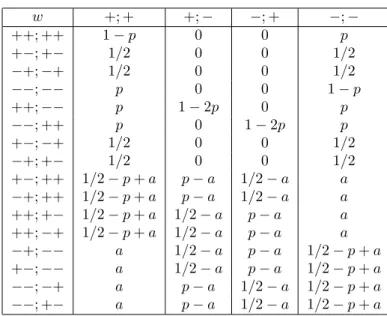
re-spectively. The resultant joint transition probabilities are displayed in Table 2 and are valid for 0 ≤ a ≤ p. For p < a≤1, the algorithm yields a joint transition probabil-ity which is independent ofaand is the one that results by formally replacing, in Table 2,abyp. The joint transition probability fulfill the following properties

X

τ′ i

w(σ′

i;τi′|σi−i, σi+1;τi−1, τi+1) =wDW(σi′|σi−i, σi+1),

(20)

X

σ′ i

w(σ′

i;τi′|σi−i, σi+1;τi−1, τi+1) =wDW(τi′|τi−1, τi+1),

(21) which reflects the condition that the system and the replica follow their own dynamics independent of the coupling.

The joint transition probabilities satisfy also the follow-ing properties. (a) Reflection symmetry in which the states of sitesi−1andi+1are interchanged, that is,σi−1↔σi+1

andτi−1↔τi+1. (b) System-replica symmetry in which the

states of the system and the replica are interchanged, that is, σi↔τifor all sites. (c) Up-down symmetry defined by the

transformationσi ↔ −σiandτi ↔ −τifor all sites.

The Hamming distance, which characterizes the damage spreading, is defined by

Ψ = 1

2h1−σiτii, (22)

which is also the order parameter related to the damage spreading phase transition.

IV

Relation with the DK automaton

In this section we show an exact relation between the stochastic dynamics defined in Section III and the DK prob-abilistic cellular automaton [9]. If we letηi be the

occupa-tion variable attached to sitei, that is,ηi= 0or1according

to whether siteiis empty or occupied by one particle, then the transition probabilities wDK(η′i|ηi−1, ηi+1)of the DK

cellular automaton is given by

wDK(1|00) = 0, (23)

wDK(1|01) =wDK(1|10) =p1, (24)

wDK(1|11) =p2. (25)

The DK cellular automaton displays a critical line in the phase diagram p1 versus p2 that separates the absorbing

state, for which the density of particles is zero, and the active state, for which the density is nonzero.

Now, let us denote byηi the coupling variable

associ-ated to the dynamics of Section III that takes the value1or

0according whetherσi 6=τiorσi =τirespectively, given

by

ηi=

1

2(1−σiτi). (26)

The relation between the Hamming distance and the cou-pling variables is just

Ψ =hηii. (27)

The joint transition probabilities in the variablesηi andσi

are defined by

˜

w(σ′

i;ηi′|σi−i, σi+1;ηi−1, ηi+1) =

=w(σ′

i;τi′|σi−i, σi+1;τi−1, τi+1), (28)

whereτi=σi(1−2ηi)

Summing over the coupling variable we get the follow-ing property

X

η′ i

˜

w(σ′

i;η′i|σi−i, σi+1;ηi−1, ηi+1) =wDW(σi′|σi−i, σi+1),

Table 2. Joint transition probabilities for the coupled system

w +; + +;− −; + −;−

++; ++ 1−p 0 0 p

+−; +− 1/2 0 0 1/2

−+;−+ 1/2 0 0 1/2

−−;−− p 0 0 1−p

++;−− p 1−2p 0 p

−−; ++ p 0 1−2p p

+−;−+ 1/2 0 0 1/2

−+; +− 1/2 0 0 1/2 +−; ++ 1/2−p+a p−a 1/2−a a

−+; ++ 1/2−p+a p−a 1/2−a a

++; +− 1/2−p+a 1/2−a p−a a

++;−+ 1/2−p+a 1/2−a p−a a

−+;−− a 1/2−a p−a 1/2−p+a

+−;−− a 1/2−a p−a 1/2−p+a

−−;−+ a p−a 1/2−a 1/2−p+a

−−; +− a p−a 1/2−a 1/2−p+a

main property we wish to show, however, is that for infinite temperature, that is, forp= 1/2we have

X

σ′ i

˜

w(σ′

i;ηi′|σi−i, σi+1;ηi−1, ηi+1) =wDK(ηi′|ηi−i, ηi+1),

(30) with the DK transition probabilites defined byp2 = 0and

p1= 1−2a. This means that the subsystem defined by the

variables{ηi}follows a dynamics identical to the DK

prob-abilistic cellular automaton. From relation (27) it follows that the Hamming distance coincides with the order param-eter of the active state displayed by the DK automaton.

Yet for the casep= 1/2, it is easy to show that the joint transition probability satisfies the property

˜

w(σ′

i;ηi′|σi−i, σi+1;ηi−1, ηi+1) =

=wDW(σ′i|σi−i, σi+1)wDK(η′i|ηi−i, ηi+1), (31)

with the DK transition probabilites defined byp2 = 0and

p1 = 1 − 2a. Therefore, the σ-subsystem and the

η-subsystem are statistically independent.

V

Mean-field solution

The dynamic mean-field approximation has already been used to study systems in nonequilibirum stationary states [6, 7, 12, 27]. Here we set up equations for an approximate solution of the equation that governs the time evolution of the coupled system. We start by writing down the equations that give the time evolution of the one-site and two-site prob-abilities, namely,

Pℓ+1(σ1;τ1) = X

σ0,σ2 X

τ0,τ2

w(σ1;τ1|σ0, σ2;τ0, τ2)

×Pℓ(σ0, σ2;τ0, τ2) (32)

and

Pℓ+1(σ1, σ3;τ1, τ3) = X

σ0,σ2.σ4 X

τ0,τ2,τ4

w(σ1;τ1|σ0, σ2;τ0, τ2)

×w(σ3;τ3|σ2, σ4;τ2, τ4)Pℓ(σ0, σ2, σ4;τ0, τ2, τ4). (33)

From now on we will drop the subscriptℓand use the prime for quantities calculated at timeℓ+ 1. To obtain a set of closed equations we use the approximation

P(σ0, σ2, σ4;τ0, τ2, τ4) =

= 1

P(σ2;τ2)

P(σ0, σ2;τ0, τ2)P(σ2, σ4;τ2, τ4), (34)

which defines the dynamic mean-field pair approximation. The probabilities P(σ1;τ1) and P(σ1, σ3;τ1, τ3)

can-not be considered all independent variables. Taking into account that they should have the reflection symmetry and the system-replica symmetry and, in addition, assuming the up-down symmetry the probabilities are related as follows

P(−; +) =P(+;−) = 1

2Ψ, (35)

P(−;−) =P(+; +) = 1

2Ω, (36)

P(−−;−−) =P(++; ++) =A, (37) P(+−;−−) =P(−+;−−) =P(−−; +−) = =P(−−;−+) =P(−+; ++) =P(+−; ++) =

=P(++;−+) =P(++; +−) =B, (38) P(−+;−+) =P(+−; +−) =C, (39) P(−−; ++) =P(++;−−) =D, (40) P(−+; +−) =P(+−;−+) =E. (41) These seven variables are not yet independent. Only three of them can be considered independent which we choose to be

Ψ,B, andD. The others are related to them by the relations

A=P(++)−2B−D, (43) C=1

2 −P(++)− 1

2Ψ +D, (44)

E=1

2Ψ−2B−D, (45)

whereP(+)andP(++)are the one-site and two-site prob-abilities corresponding to a single system. The exact equi-librium solution of the one-dimensional Ising model gives P(+) = 1/2andP(++) = [1 + (tanhβJ)2_]/4.

From the time evolution given by Eqs. (32) and (33) and using Eqs. (43), (44), and (45) we obtain the following closed equations forΨ,D, andB

Ψ′_{= 2γD+ 8αB, (46)}

D′ _{= 4α}2B2

Ω + (4α

2_+γ2₎B2

Ψ+

+2γ(γ+ 2α)DB Ψ + 2γ

2D2

Ψ, (47)

B′_{= 2αB−4α}2B2

Ω −4α

2B2

Ψ −2αγ

DB

Ψ , (48)

where

γ= 1−2p (49)

and

α= 1

2+p−2a. (50)

0.1 0.2 0.3 0.4 0.5

p

0 0.05 0.1 0.15 0.2

a

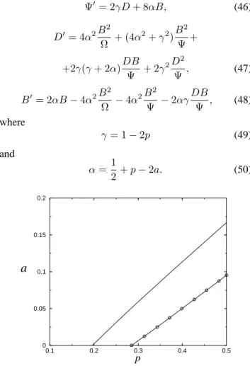
Figure 1. Phase diagram in the planea versuspwherepis re-late to temperature by (8). The continuous line corresponds to the mean-field approximantion and the circles to the Monte Carlo sim-ulations.

A stationary solution of the evolution equation is such that the stationary probabilityP(σ;τ)is zero whenσ 6=τ which corresponds to no damage spreading (Ψ = 0). From Eqs. (46), (47), and (48) we may obtain solutions with dam-age spreading (Ψ6= 0). The transition line is obtained by a linear stability analysis of the solution aroundΨ = 0and by assuming that the variablesBandDvanishes linearly with

Ψ. Taking the limitΨ→0we find a transition line given by the implicit equation

(1−α)2γ3−4α(3α2−5α+ 2)γ2+

+4α2(13α2−16α+ 5)γ−8α(3α−2) = 0, (51) whose solution is shown in the phase diagram of Fig. 1. In particular, whena= 0(corresponding to the HD algorithm) we haveγ= 2(1−α)which substituted in the equation for the transition line gives

1−9α+ 33α2−59α3+ 53α4−20α5= 0, (52) whose solution isα = 0.696173from which we getp = 0.196173so thatJ/kBTc = 0.352597andTc = 2.83610.

Whena= 1/2(correspoding to the HB algorithm) there is no transition.

At infinite temperature,p= 1/2, the mean-field transi-tion line givesa= 1/6. Now, using the relationp1= 1−2a

obtained from the equivalence with the DK automaton, and taking into account the result p1 = 2/3 obtained in [12]

in the pair approximation for the DK automaton we have a= 1/6in coincidence with our present result.

VI

Numerical simulations

Our numerical simulations resulted in the transition line shown in Fig. 1. When a = 0 we have obtained p = 0.285(1) which gives J/kBTc = 0.230(1) and Tc =

4.35(2)in agreement with the result by Hinrichsen and Do-many [15], namelyJ/kBTc = 0.2305. At infinite

temper-ature, p = 1/2, the numerical results give a transition at a = 0.0955(1). Now, using the relationp1 = 1−2a

ob-tained from the mapping of our model to the DK cellular au-tomaton, we obtainp1c = 0.809(1)in agreement with

previ-ous Monte Carlo numerical results, namelyp1c= 0.8095(5)

[28].

2 4 6 8

lnt

−2 −1.8 −1.6 −1.4 −1.2 −1

lnΨ

Figure 2. Time dependent Monte Carlo simulations for the dam-age survival probabilityP for a lattice with linear sizeL= 1000_. Numerical data are shown fora = 0_.075_andp= 0_.450_,0_.453_, 0_.455_,0_.457_{, and}0_.460_{from bottom to top.}

random number for both lattices. The density of damages

Ψ(t), obtained by taking the averages over 2000 samples, were collected fromt= 1tot = 1500Monte Carlo steps. At the critical point we expect the following asymptotic time behavior [22]

Ψ(t)∼t−δ_{. (53)}

Therefore, a double-log plot ofΨversustwill be linear at the critical point. In Fig. 2 we show how the critical value of pwas found whena = 0.075. Several values ofp, the ones shown in Fig. 2, were checked in order to find a linear behavior in a log-log plot ofΨversust. Our estimate in this case givespc = 0.455(1)fora = 0.075. The straight line

fitted to the numerical data givesδ= 0.16(1)in agreement with a transition belonging to the direct percolation univer-sality class [7]. For other values ofathe procedure was the same.

VII

Conclusion

We have introduced a family of algorithms to describe the time evolution of the one-dimensional Ising model The fam-ily of algorithms interpolates between the HB and the HD al-gorithms and the resulting stochastic dynamics corresponds to the DW probabilistic cellular automaton. Coupling a sys-tem with its replica by using the same sequence of random numbers, we have determined the joint transition probabil-ity which defines a four-state probabilistic cellular automa-ton. By using a dynamic pair mean-field approximation and Monte Carlo simulations we have found that the stochas-tic dynamics defined by the family of algorithms displays a line of critical points separating a phase where the damage spreads and a phase where it does not. One important fea-ture of the joint stochastic dynamics studied here is that at infinite temperature the joint dynamics is exactly mapped into the DK probabilistic cellular automaton. This result together with the Monte Carlo simulations give support to a conjecture by Grassberger according to which the dam-age spreading transition is in the universality class of the directed percolation.

References

[1] R. J. Glauber, J. Math. Phys. 4, 294 (1963).

[2] Monte Carlo Methods in Statistical Physics, edited by K. Binder, 2nd. ed. (Springer-Verlag, Berlin, 1986).

[3] K. Kawasaki in Phase Transitions and Critical Phenomena, edited by C. Domb and M. S. Green (Academic Press, New York, 1972), vol. 2, p. 443.

[4] N. G. van Kampen, Stochastic Process in Physics and

Chem-istry (North-Holland, Amsterdam, 1981).

[5] T. M. Liggett, Interacting Particle Systems (Spinger-Verlag, New York, 1985).

[6] T. Tom´e and M. J. de Oliveira, Phys. Rev. A 40, 6643 (1989).

[7] J. Marro and R. Dickman, Nonequilibrium Phase Transition

in Lattice Models (Cambridge University Press, Cambridge,

1999).

[8] T. Tom´e e M. J. de Oliveira, Dinˆamica Estoc´astica e

Irre-versibilidade (Editora da Universidade de S˜ao Paulo, S˜ao

Paulo, 2001).

[9] E. Domany and W. Kinzel, Phys. Rev. Lett. 53, 447 (1984).

[10] B. Derrida and G. Weisbuch, Europhys. Lett. 4, 657 (1987).

[11] J. L. Lebowitz, C. Maes and E. R. Speer, J. Stat. Phys. 59, 117 (1990).

[12] T. Tom´e, Physica A 212, 99 (1994).

[13] E. P. Gueuvoghlanian and T. Tom´e, Int. J. Mod. Phys. B 11, 1245 (1997).

[14] M. N. Barber and B. Derrida, J. Stat. Phys. 51, 877 (1988).

[15] H. Hinrichsen and E. Domany, Phys. Rev. E 56, 94 (1997).

[16] T. Tom´e and M. J. de Oliveira, Braz. J. Phys. 27, 525 (1997).

[17] M. J. de Oliveira, Int. J. Mod. Phys. B 10, 1313 (1996).

[18] P. Grassberger, Physica A 214, 547 (1995).

[19] M. Creutz, Ann. Phys. 167, 62 (1986).

[20] H. Stanley, D. Stauffer, J. Kertesz, and H. Herrmann, Phys. Rev. Lett. 59, 2326 (1987).

[21] A. M. Mariz, H. J. Hermann, and L. de Arcangelis, J. Stat. Phys. 59, 1043 (1990).

[22] P. Grassberger, J. Stat. Phys. 79, 13 (1995).

[23] H. Hinrichsen, J. S. Weitz and E. Domany, J. Stat. Phys. 88, 617 (1997).

[24] E. Arashiro and J. R. Drugowich de Fel´ıcio, Braz. J. Phys. 30, 677 (2000).

[25] M. L. Martins, H. F. Verona de Rezende, C. Tsallis and A. C. N. de Magalh˜aes, Phys. Rev. Lett. 66, 2045 (1991).

[26] P. Grassberger and A. de la Torre, Ann. Phys. (NY) 122, 373 (1979).

[27] R. Dickman, Phys. Rev. A 34, 4246 (1986).