It is important to evaluate which designing models are safe and appropriate to structural analysis of buildings constructed in Concrete Wall system. In this work it is evaluated, through comparison of maximum normal stress of compression, a simple numerical model, which represents the walls with frame elements, with another much more robust and reined, which represents the walls with shells elements. The designing of the normal stress of compression it is done for both cases, based on NBR 16055, to conclude if the wall thickness initially adopted, it is enough or not.
Keywords: reinforced concrete walls; numerical models; normal stress of compression.
É fundamental se conhecer quais modelos numéricos são seguros e pertinentes para a análise estrutural de ediicações construídas pelo siste -ma Paredes de Concreto. Neste trabalho é avaliado, por meio da comparação da máxi-ma tensão nor-mal de compressão, um modelo numérico mais simples, que discretiza as paredes em elementos de barra, com outro mais robusto e reinado que discretiza as paredes com elementos de casca. A veriicação do dimensionamento da máxima tensão normal de compressão é realizada para os dois casos, considerando as premissas da norma brasileira NBR 16055 a im de concluir se a espessura das paredes adotada inicialmente é suiciente ou não.
Palavras-chave: paredes de concreto armado; modelos numéricos; tensão normal de compressão.
Design of reinforced concrete walls casted in place
for the maximum normal stress of compression
Dimensionamento de paredes de concreto armado
moldadas no local para a máxima tensão normal
de compressão
T. C. BRAGUIM a [email protected]
T. N. BITTENCOURT a [email protected]
a Departamento de Engenharia de Estruturas e Geotécnica, Escola Politécnica da Universidade de São Paulo, São Paulo, Brasil.
Received: 15 Nov 2013 • Accepted: 12 Mar 2014 • Available Online: 02 Jun 2014
Abstract
1. Introduction
Since 2007, a signiicant use of the system known as Concrete Wall has been inluenced the Brazilian residential construction market. In April 2012, a Brazilian code exclusively devoted to this system was published. Besides that, the challenge in reducing housing deicit stimulate the use of this alternative method, because when properly applied it provides high productivity and lower costs com-pared with other construction methods. As it is a constructive meth-od which the main concept brings the idea of the industrialization of the construction, it is important to highlight that it is necessary to considerer the time for the structure execution (one vantage of the Concrete Wall System because it is considered fast), to make a re-alistic comparison of costs between it and the conventional method or the structure masonry, for instance. In terms of structural design it is important to evaluate which designing models are safe and appropriate to structural analysis of buildings constructed in Con-crete Wall System. This work presents the comparison of results between some possible numerical models to design a concrete wall for the maximum normal stress of compression, as the recent Brazilian code NBR 16055:2012 - Concrete wall castes in place for building construction – Requirements and proceedings [4].
1.1 Initial consideration
In the structural design of buildings constructed by Concrete Walls system, the thickness of the walls is one of the main settings to be made. This deinition involves several variables such as, the height of the building, the external forces acting in it, the resistance of the materials used and the assumptions of how these walls are represented numerically.
Normally the walls of a building of concrete walls are subjected to normal compressive stresses that are superior on the normal tensile and shear stresses. Thus, the deinition of wall thickness is made by comparing the maximum normal stress of compres-sion with the ultimate normal stress of comprescompres-sion according with some code.
1.2 Aims
This study aims to compare the maximum normal stress of com-pression in the critical cross section of the concrete walls of a build-ing, obtained by two different numerical models, and verify it with the ultimate strength of compression calculated by the NBR 16055 [4]. From the comparison of results is a purpose evaluate the qual-ity of the simpler model over more reined model and see if the wall thickness adopted initially is suficient.
1.3 Method
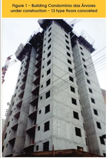
It was used as a study case, the building Condomínio das Árvores, built in 2012 in São Bernado do Campo by construction Sergus Construções e Comércio Ltda.
The building was modeled using the inite element method. The irst model, called Finite Element Model (MEF), and taken as a ref-erence model for the comparison of results to be the most reined, represents the walls with shell Tridimensional Frame Model (MPT). First, the distribution of vertical loads on the walls is done according to each numerical model. The concentrated characteristic normal
force, obtained only by vertical loads, is compared between the models at the foundation level, in order to verify the differences. Then the characteristic normal forces and bending moments ob -tained from some walls, considering only horizontal actions, are compared through their diagrams.
The combination of vertical and horizontal actions is done to obtain the maximum normal stress of compression. This result is compared between the two models on some walls of the studied building. Finally, it is calculated the ultimate strength of compression using the expression given in NBR 16055 [4], and it is checked whether the thickness of the walls of the building studied initially adopted, it is enough to resist to normal stresses of compression.
It is noteworthy that the NBR 16055 [4] covers concepts that go beyond the NBR 6118:2007 - Design of concrete structures - Pro-cedures [1], such as the deinition of concrete wall. According to NBR 16055 [4], in item 14.4, a concrete wall is deined when the length of the wall is greater than or equal to ten times its thickness. The NBR 6118 [1] deines pillar-wall, on your item 14.4.2.4, when the largest cross-sectional dimension of a pillar is greater than or equal to 5 times their smaller size. Another observation is that this paper brings a study of walls, and not wall-beams. That means that the concrete walls analyzed have continuous support throughout your base, unlike the wall-beams that have discrete support. The numerical models (FEM and MPT) were developed in
SAP2000 software - version 15, based on the Finite Element Meth -od, considering linear elastic analysis. The interaction between soil and structure was not considered.
2. Study case
It was used an adaptation of the building Condomínio das Árvores of the enterprise Reserva Jardim Botânico, built in the city of São Ber-nardo do Campo, in 2012, by the construction Sergus Construções e Comércio Ltda, as shown in Figure [1]. The structural design was provided by OSMB Engineers and Associates S / S Ltda.
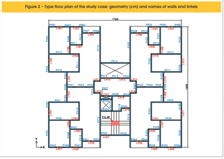
The geometry of the building was adapted in relation to the building constructed in order to simplify the numerical modeling. Howev-er, its main features have been retained. All measurements were multiple of 40 cm, and the number of loors was adopted equal to ifteen types, thus not having the transition from the ground to the irst loor and the attic, provided for in the original design. It was considered the distance between loors of 2.80 m. The Figure [2] shows the type loorplan with walls and lintels (regions above and below doors and windows) of reinforced concrete, named as the horizontal and vertical directions. Though the massive concrete slabs are not named in Figure [2], they were considered in the whole loorplan, with a thickness of 10 cm, except in pressuriza -tion, lift and installations openings, where a hole is represented
by X . The stairwell was considered to be a massive slab of 10 cm thick. The only pillar in the structure is also made with reinforced concrete and it is located at the middle of the stairwell. In the loor -plan it is represented by a hatch in red.
3. Loads considered
3.1 Vertical loads
The vertical loads considered were the permanent loads (dead loads) and the accidental loads (live loads) according to NBR 6120 [2]. For that were considered:
n own weight for the structure elements:
γ
= 250 kN/m3;n permanent loads (dead loads): L
g
= 1,0 kN/m2;n accidental loads (live loads): L
q
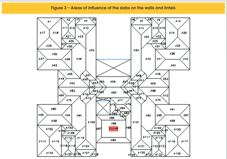
= 1,5 kN/m2.To calculate the reactions of slabs on the walls, it was used the method of plastic hinges which is based in the approximate posi-tion of the break lines that deine the areas of inluence of the slabs on the walls.
Figure [3] shows the areas of inluence of the slabs to unload their loads in walls and lintels by the method of plastic hinges.
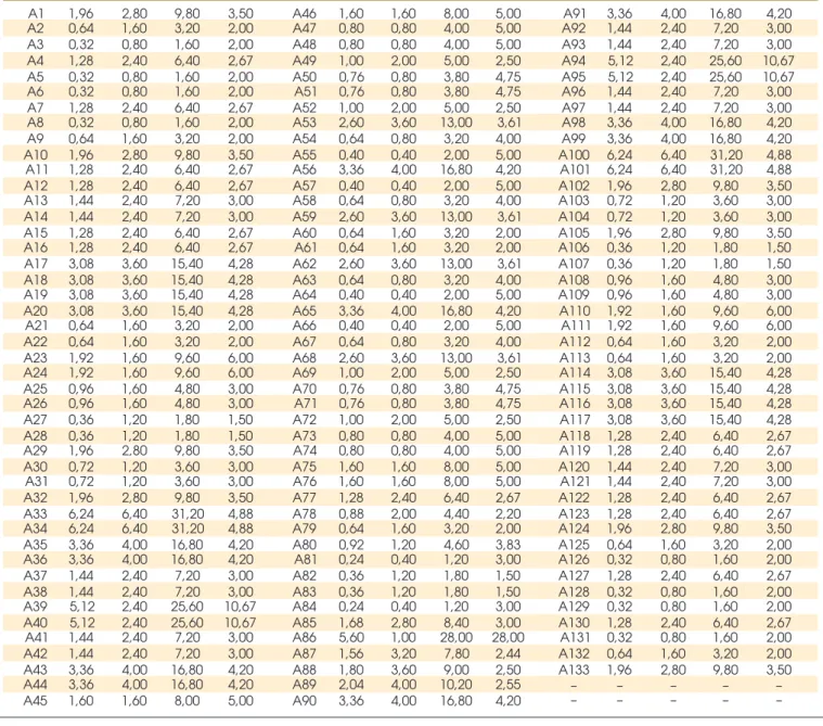
The values of the areas of inluence (
A
L), lengths of inluence (L
inf), along which the load of their area of inluence is distributed in the walls and/or lintels and the concentrated loads (P) anded loads (p), acting in the length of inluence, are shown in Table [1]. Corrêa and Ramalho [7] reported that the deinition of how the ac-tion of the slabs on the walls that serve as support takes place, and also how interactions occur between walls, are crucial to obtain a coherent structural analysis aspects of the walls.
3.2 Horizontal loads
This work was just considered horizontal loads due to wind and out of plumb load, centered.
The ABNT NBR 6123:1988 - Forces due to wind on buildings [5], allows to transform the wind pressures that fall perpendicularly on the surface of the walls in static forces. For this it is necessary to deine the characteristic wind speed as shown in Equation [1]:
(1)
3 2 1 0
.
S
.
S
.
S
v
v
k=
where
v
k is the characteristic wind velocity (m/s),v
0 is the basic wind speed (m/s),S
1 is the topographic factor,S
2 is the factorwhich considers the roughness of the terrain and the variation of wind speed with the height of a building and its dimensions in plan and
S
3 is the statistical factor.The dynamic wind pressure
q
vento (N/m2) is determined by the characteristic wind velocity as pointed in item 4.2 of NBR 6123 [5], described in Equation [2]:(2)
2613
,
0
kvento
v
q
=
Finally the drag force which is the component of the global wind force in a given direction is deined by Equation [3]:
(3)
e vento a
a
C
q
A
F
=
.
.
in which,
F
a is the drag force in the direction of the wind,a
C
is the drag coefficient as wind direction andA
e is the effective frontal area on a plane perpendicular to the wind direction.The out of plumb caused by eccentricities arising from con-struction of a building is considered in the structure by horizon-tal loads equivalents to this displacements. As indicated in the NBR 16055 [4] for multi-story buildings, must be considered a
global out of plumb through an angle of out of plumb, calcu-lated by Equation [4]:
(4)
H
.
170
1
=
q
where,
θ
is the angle of out of plumb (rad) and H is the total height of the building (m).The equation [5] transform the effect of the out of plumb into an equivalent horizontal force (
F
dp) in terms ofθ
and total vertical load on the loor, represented by∆
P
.(5)
q
.
P
F
dp=
D
Table 1 – Values o
f the areas of influence of the slabs on the walls and lintels and their respective loads
Area of influence and loads from the slabs
Area A (m ) L inf (m) P (kN) p (kN/m)2 Area A (m ) L inf (m) P (kN) p (kN/m)2 Area A (m ) L inf (m) P (kN) p (kN/m)2
A1 1,96 2,80 9,80 3,50 A46 1,60 1,60 8,00 5,00 A91 3,36 4,00 16,80 4,20
A2 0,64 1,60 3,20 2,00 A47 0,80 0,80 4,00 5,00 A92 1,44 2,40 7,20 3,00
A3 0,32 0,80 1,60 2,00 A48 0,80 0,80 4,00 5,00 A93 1,44 2,40 7,20 3,00
A4 1,28 2,40 6,40 2,67 A49 1,00 2,00 5,00 2,50 A94 5,12 2,40 25,60 10,67
A5 0,32 0,80 1,60 2,00 A50 0,76 0,80 3,80 4,75 A95 5,12 2,40 25,60 10,67
A6 0,32 0,80 1,60 2,00 A51 0,76 0,80 3,80 4,75 A96 1,44 2,40 7,20 3,00
A7 1,28 2,40 6,40 2,67 A52 1,00 2,00 5,00 2,50 A97 1,44 2,40 7,20 3,00
A8 0,32 0,80 1,60 2,00 A53 2,60 3,60 13,00 3,61 A98 3,36 4,00 16,80 4,20
A9 0,64 1,60 3,20 2,00 A54 0,64 0,80 3,20 4,00 A99 3,36 4,00 16,80 4,20
A10 1,96 2,80 9,80 3,50 A55 0,40 0,40 2,00 5,00 A100 6,24 6,40 31,20 4,88
A11 1,28 2,40 6,40 2,67 A56 3,36 4,00 16,80 4,20 A101 6,24 6,40 31,20 4,88
A12 1,28 2,40 6,40 2,67 A57 0,40 0,40 2,00 5,00 A102 1,96 2,80 9,80 3,50
A13 1,44 2,40 7,20 3,00 A58 0,64 0,80 3,20 4,00 A103 0,72 1,20 3,60 3,00
A14 1,44 2,40 7,20 3,00 A59 2,60 3,60 13,00 3,61 A104 0,72 1,20 3,60 3,00
A15 1,28 2,40 6,40 2,67 A60 0,64 1,60 3,20 2,00 A105 1,96 2,80 9,80 3,50
A16 1,28 2,40 6,40 2,67 A61 0,64 1,60 3,20 2,00 A106 0,36 1,20 1,80 1,50
A17 3,08 3,60 15,40 4,28 A62 2,60 3,60 13,00 3,61 A107 0,36 1,20 1,80 1,50
A18 3,08 3,60 15,40 4,28 A63 0,64 0,80 3,20 4,00 A108 0,96 1,60 4,80 3,00
A19 3,08 3,60 15,40 4,28 A64 0,40 0,40 2,00 5,00 A109 0,96 1,60 4,80 3,00
A20 3,08 3,60 15,40 4,28 A65 3,36 4,00 16,80 4,20 A110 1,92 1,60 9,60 6,00
A21 0,64 1,60 3,20 2,00 A66 0,40 0,40 2,00 5,00 A111 1,92 1,60 9,60 6,00
A22 0,64 1,60 3,20 2,00 A67 0,64 0,80 3,20 4,00 A112 0,64 1,60 3,20 2,00
A23 1,92 1,60 9,60 6,00 A68 2,60 3,60 13,00 3,61 A113 0,64 1,60 3,20 2,00
A24 1,92 1,60 9,60 6,00 A69 1,00 2,00 5,00 2,50 A114 3,08 3,60 15,40 4,28
A25 0,96 1,60 4,80 3,00 A70 0,76 0,80 3,80 4,75 A115 3,08 3,60 15,40 4,28
A26 0,96 1,60 4,80 3,00 A71 0,76 0,80 3,80 4,75 A116 3,08 3,60 15,40 4,28
A27 0,36 1,20 1,80 1,50 A72 1,00 2,00 5,00 2,50 A117 3,08 3,60 15,40 4,28
A28 0,36 1,20 1,80 1,50 A73 0,80 0,80 4,00 5,00 A118 1,28 2,40 6,40 2,67
A29 1,96 2,80 9,80 3,50 A74 0,80 0,80 4,00 5,00 A119 1,28 2,40 6,40 2,67
A30 0,72 1,20 3,60 3,00 A75 1,60 1,60 8,00 5,00 A120 1,44 2,40 7,20 3,00
A31 0,72 1,20 3,60 3,00 A76 1,60 1,60 8,00 5,00 A121 1,44 2,40 7,20 3,00
A32 1,96 2,80 9,80 3,50 A77 1,28 2,40 6,40 2,67 A122 1,28 2,40 6,40 2,67
A33 6,24 6,40 31,20 4,88 A78 0,88 2,00 4,40 2,20 A123 1,28 2,40 6,40 2,67
A34 6,24 6,40 31,20 4,88 A79 0,64 1,60 3,20 2,00 A124 1,96 2,80 9,80 3,50
A35 3,36 4,00 16,80 4,20 A80 0,92 1,20 4,60 3,83 A125 0,64 1,60 3,20 2,00
A36 3,36 4,00 16,80 4,20 A81 0,24 0,40 1,20 3,00 A126 0,32 0,80 1,60 2,00
A37 1,44 2,40 7,20 3,00 A82 0,36 1,20 1,80 1,50 A127 1,28 2,40 6,40 2,67
A38 1,44 2,40 7,20 3,00 A83 0,36 1,20 1,80 1,50 A128 0,32 0,80 1,60 2,00
A39 5,12 2,40 25,60 10,67 A84 0,24 0,40 1,20 3,00 A129 0,32 0,80 1,60 2,00
A40 5,12 2,40 25,60 10,67 A85 1,68 2,80 8,40 3,00 A130 1,28 2,40 6,40 2,67
A41 1,44 2,40 7,20 3,00 A86 5,60 1,00 28,00 28,00 A131 0,32 0,80 1,60 2,00
A42 1,44 2,40 7,20 3,00 A87 1,56 3,20 7,80 2,44 A132 0,64 1,60 3,20 2,00
A43 3,36 4,00 16,80 4,20 A88 1,80 3,60 9,00 2,50 A133
– – – – –
– – – – –
1,96 2,80 9,80 3,50 A44 3,36 4,00 16,80 4,20 A89 2,04 4,00 10,20 2,55
4. Numerical models
4.1 Finite element model
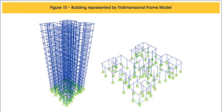
The Finite Element Model named in this work refers to the repre-sentation of the walls of the building analyzed in square plane shell elements, with nodes only at the vertices. It was used the shell
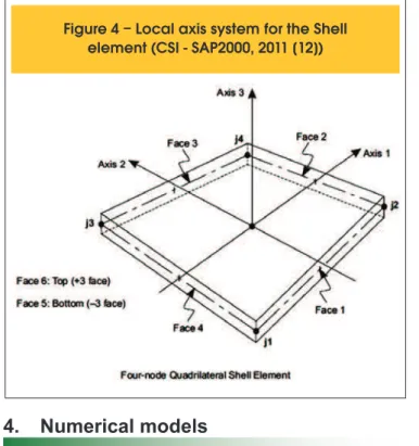
element from software SAP2000 for such modeling, with dimensions 40 cm x 40 cm and thickness as the same as the wall, adopted equal to 12 cm. The system of local axes of the element and its four nodes are shown in Fig. [4]. The degrees of freedom for the element node are shown in Figure [5]. The slabs were not represented, and to simulate its behavior, it was used the tool rigid diaphragm. Figure [6] shows the Finite Element Model of the studied building.
4.2 Tridimensional frame model
The Tridimensional Frame Model, named by Nascimento Neto [8],
Figure 4 – Local axis system for the Shell
element (CSI - SAP2000, 2011 [12])
certain finite element (CSI - SAP2000, 2011 [12])
e 5 – Degrees of freedom for the node at
is an adaptation of a model proposed by Yagui [11], which makes the representation of hard-core in bar elements, horizontally re-stricted by slabs acting as a rigid diaphragm.
The adaptation of Yagui [11] model proposed by Nascimento Neto [8] and called Tridimensional Frame Model has small changes in the formulation of the element, making it more comprehensive. Moreover, its application has been made in structural systems composed of walls, as in the case of buildings constructed in Struc-tural Masonry and Concrete Walls. Nunes [10] used the
Tridimen-sional Frame Model to analyze the internal forces of a building of concrete walls, as well as Nascimento Neto [8] evaluated for the case of Structural masonry.
Unlike Yagui model, the Tridimensional Frame Model considers the lexural rigidity in the direction of lower inertia of the wall, be-cause it is modeled by three-dimensional bar with six degrees of freedom at each end. However, the layout and some features of the bars in the Tridimensional Frame Model, are the same as in Yagui model, i.e.:
Figure 7 – Tridimensional Frame Model (CORRÊA, 2003 [6])
Visão em planta
BB
Visão em perspectivaA
F
igure 8 – Application of Tridimensional Frame Model
Walls and lintels with “full” cross-section Tridimensional vertical and horizontal bars
n a lexible vertical bar is positioned at the vertical axis of the wall
having the elastic and geometric features that replaces the wall segment;
n beyond the bending deformation, the shear deformation is
con-sidered in lexible vertical bars;
n horizontal rigid bars are arranged at loor level and connect the
ends of the walls to the lexible vertical bar; the height and width of the cross section is equal to the wall that the bar represents;
n the endpoints nodes of the horizontal rigid bars are articulated
(except when the end is connected to a lintel or other rigid hori-zontal bar collinear), and the common node to the lexible verti -cal bar is continuous;
n horizontal rigid bars have ininite lexural rigidity in the plane and
simulate the length of the walls and the interaction between them. It is important to consider the shear deformation in the verti-cal bar elements due to the relatively large dimensions of the walls when compared to a beam, for example. According to NBR 16055 [4], in item 14.3, for the consideration of the wall as a structural bracing system, represented by linear element component, it is necessary to consider besides the bending de-formation, the shear deformation. The horizontal bars are rigid and therefore such deformation is not considered therein. The Tridimensional Frame Model is shown in Figure [7]. As Nascimento and Corrêa [9], the walls that intersect are in-terlinked / connected by horizontal rigid bars, in order to con -sider the interaction that effectively develops between walls, which is simulated by the shear that arises in the intersection node. Thus, the horizontal rigid bars that are not collinear, has its endpoint node articulated which is as well an intersection node. So the only degree of freedom associated to this node is vertical translation.
The inclusion of lintels is also possible in this model, which greatly increases the rigidity of the building. When taken, it is necessary that the connection between the lintel and the rigid horizontal bar is continuous so as to simulate a real contribution. Figure [8] shows an application of the Tridimensional Frame
Model to illustrate some of its features. In Figure [8a], walls and lintels are presented with their “full” cross sections. In Figure [8b], it is observed the three-dimensional vertical and horizontal bars, with their names. Analyzing the ends of the horizontal bars not collinear, it is noted that they have been articulated (the joint is represented by a green circle). It is also evident that the con-tinuity between horizontal rigid bars and lintels was maintained (example: connecting the bar 102 to bar 5). There was also con-tinuity in meeting vertical bars with horizontal bars (example: connecting the bar 1 with bars 101 and 102).
It is important to remember that as the wall is represented by a vertical bar which has the geometrical characteristics of the wall and horizontal bars having the same height and thickness of the wall and simulate its length, it is necessary to disregard the own weight of the horizontal bars. Otherwise, the weight of the wall would be counted twice.
In studies carried out in this work, it was multiplied by 100 the bending stiffness of the major inertia direction of the horizontal rigid bar in order to make them infinitely rigid in the plane of the wall.
The hypothesis of the slabs acting as a rigid diaphragm is also considered in the Tridimensional Frame Model. Thus, the initial and inal nodes of the vertical bars are linked to the respective loor master node. Thus, in the six degrees of freedom at each end of the vertical bar, three are “slaves” to the master node of the loor, which are related to the two horizontal translations and rotation about the longitudinal axis of the vertical bar.
As previously mentioned, the Tridimensional Frame Model was developed by the inite element method in commercial software SAP2000. To represent the horizontal rigid bars and vertical lexible bars rigid bars, it was used the frame element from the library of elements of the program, which formulation is as Bathe e Wilson apud CSI [12]. The shear deformation is considered in this formulation, however, it was not considered in the horizontal rigid bars. The system of axes of the local frame element can be seen in Figure [9] and the degrees of freedom of a node element
in Figure [5]. The Figure [10] shows the Tridimensional Frame Model applied to the studied building.
4.3 Mechanical properties of concrete
It was considered physical linearity to concrete material in both numerical model (MEF and MPT). The mechanical properties considered for the concrete material were: compression strength of 25 MPa (25000 kN/m2), secant modulus of elasticity
E
cs= 24000000 kN/m2, Poisson’s ratioν
= 0.2 and a speciic weightγ
= 250 kN/m3. The material was considered as isotropic.5. Results
5.1 Distribution of vertical loads
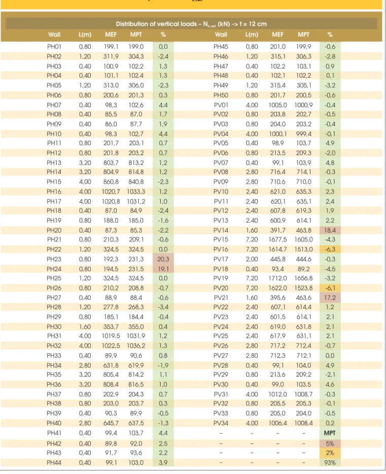
Table [2] compares the normal concentrated forces only from the vertical load (
N
k,vert), obtained by MEF and MPT at the founda-tion level models. The cells painted in green mean that the differ-ence in outcome of MPT compared to MEF is less than or equal, in absolute value, than 5%, showing an excellent approximation. Those painted in yellow mean that the difference was obtained at all, greater than 5% and less than or equal to 15% range that describes the results as good value. Painted red cells show differ-ences above 15% threshold at which the result is considered bad. The 15% limit which classiies the difference in results between calculation models as poor, was based on the coeficient
γ
f3which considers the possible errors in the evaluation of the load effects, occurred by construction problems or by deiciency of the method of calculation employed. According to NBR 8681:2003 - Actions and safety of structures - Procedures [3], when consider-ing the ultimate limit states, the
γ
f coeficients can be consideredas the product of
γ
f1, considering the variability of the actionsand,
γ
f3 that can be adopted equal to 1.18. This means that theaccuracy of a model calculation can vary by up to 18% without the degree of safety of the structure is affected.
The approximation of results is very good, since 93% of the walls showed differences of less than 5%, 2% of the walls differences be-tween 5% and 15%, and only 5% of the walls showed poor result. The walls PV14 and its symmetrical PV21, and the walls PH23 and its symmetrical PH24, showed differences of
N
k,vert, between the two models analyzed, greater than 15% and up to 20.3%. The wall PH23 interacts with the wall PV14, and the wall PH24 interacts with the wall PV21 in order to standardize the vertical loads. So, each pair of these walls forms a group of walls. Note that the group of walls PH23-PV14 and PV21-PH24, are connected through lintels to much larger groups of walls, which are located in the middle of the building.The interaction between groups with high rigidity with groups of relative small stiffness, through just a lintel, may be the cause of the difference in results for these cases, however this hypothesis needs to be examined.
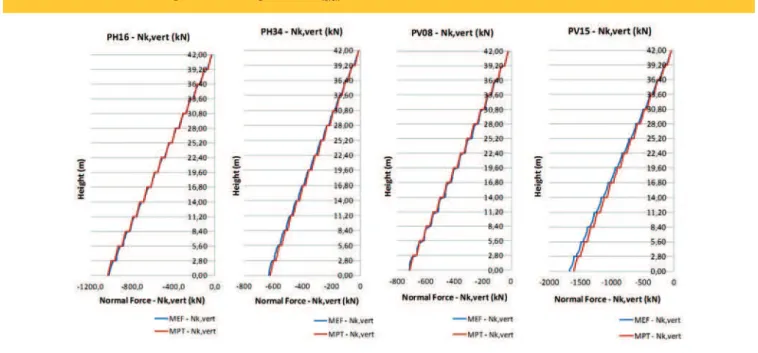
Another important factor, and that makes the MPT in favor of safety, is the fact that all the poor results in terms of normal concentrated force are higher than the normal concentrated forces obtained by MEF model. In order to show the veriication of the maximum normal compres-sive stress, and avoid excescompres-sive results, it was decided to present the diagrams of internal forces of two shear walls in the horizontal direction (PH16 and PH34) and two shear walls in vertical direction (PV08 and PV15).
Figure [11] shows the normal force diagrams, considering only the distribution of vertical loads, of the PH16, PH34, PV08 and PV15 walls. It is noted that a good approximation results between MPT and MEF models occurs along the entire height of the wall.
5.2 Bending moment and normal force due to only
horizontal actions
The following are presented and compared the bending moment
Table 2 – Comparison of
N
k,vertat the foundation level
Wall L(m) MEF MPT % Wall L(m) MEF MPT %
PH01 0,80 199,1 199,0 0,0 PH45 0,80 201,0 199,9 -0,6
PH02 1,20 311,9 304,3 -2,4 PH46 1,20 315,1 306,3 -2,8
PH03 0,40 100,9 102,2 1,3 PH47 0,40 102,2 103,1 0,9
PH04 0,40 101,1 102,4 1,3 PH48 0,40 102,1 102,2 0,1
PH05 1,20 313,0 306,0 -2,3 PH49 1,20 315,4 305,1 -3,2
PH06 0,80 200,6 201,3 0,3 PH50 0,80 201,7 200,5 -0,6
PH07 0,40 98,3 102,6 4,4 PV01 4,00 1005,0 1000,9 -0,4
PH08 0,40 85,5 87,0 1,7 PV02 0,80 203,8 202,7 -0,5
PH09 0,40 86,0 87,7 1,9 PV03 0,80 204,0 203,2 -0,4
PH10 0,40 98,3 102,7 4,4 PV04 4,00 1000,1 999,4 -0,1
PH11 0,80 201,7 203,1 0,7 PV05 0,40 98,9 103,7 4,9
PH12 0,80 201,8 203,2 0,7 PV06 0,80 213,5 209,3 -2,0
PH13 3,20 803,7 813,2 1,2 PV07 0,40 99,1 103,9 4,8
PH14 3,20 804,9 814,8 1,2 PV08 2,80 716,4 714,1 -0,3
PH15 4,00 860,8 840,8 -2,3 PV09 2,80 710,6 710,0 -0,1
PH16 4,00 1020,7 1033,3 1,2 PV10 2,40 621,0 635,3 2,3
PH17 4,00 1020,8 1031,2 1,0 PV11 2,40 620,1 635,1 2,4
PH18 0,40 87,0 84,9 -2,4 PV12 2,40 607,8 619,3 1,9
PH19 0,80 188,0 185,0 -1,6 PV13 2,40 600,9 614,1 2,2
PH20 0,40 87,3 85,3 -2,2 PV14 1,60 391,7 463,8
PH21 0,80 210,3 209,1 -0,6 PV15 7,20 1677,5 1605,0 -4,3
PH22 1,20 324,5 324,5 0,0 PV16 7,20 1614,7 1513,0
PH23 0,80 192,3 231,3 20,3 PV17 2,00 445,8 444,6 -0,3
PH24 0,80 194,5 231,5 19,1 PV18 0,40 93,4 89,2 -4,5
PH25 1,20 324,5 324,5 0,0 PV19 7,20 1712,0 1656,8 -3,2
PH26 0,80 210,2 208,8 -0,7 PV20 7,20 1622,0 1523,8
PH27 0,40 88,9 88,4 -0,6 PV21 1,60 395,6 463,6
PH28 1,20 277,8 268,3 -3,4 PV22 2,40 607,1 614,4 1,2
PH29 0,80 185,1 184,4 -0,4 PV23 2,40 601,5 614,1 2,1
PH30 1,60 353,7 355,0 0,4 PV24 2,40 619,0 631,8 2,1
PH31 4,00 1019,5 1031,9 1,2 PV25 2,40 617,9 631,1 2,1
PH32 4,00 1022,5 1036,2 1,3 PV26 2,80 717,2 712,4 -0,7
PH33 0,40 89,9 90,6 0,8 PV27 2,80 712,3 712,1 0,0
PH34 2,80 631,8 619,9 -1,9 PV28 0,40 99,1 104,0 4,9
PH35 3,20 805,4 814,2 1,1 PV29 0,80 213,6 209,2 -2,1
PH36 3,20 808,4 816,5 1,0 PV30 0,40 99,0 103,5 4,6
PH37 0,80 202,9 204,3 0,7 PV31 4,00 1012,0 1008,7 -0,3
PH38 0,80 203,0 203,7 0,3 PV32 0,80 205,5 205,3 -0,1
PH39 0,40 90,3 89,9 -0,5 PV33 0,80 205,0 204,0 -0,5
PH40 2,80 645,7 637,5 -1,3 PV34 4,00 1006,4 1008,4 0,2
PH41 0,40 99,4 103,7 4,4 – – – –
– – – –
– – – –
– – – –
MPT
PH42 0,40 89,8 92,0 2,5
PH43 0,40 91,7 93,6 2,2
PH44 0,40 99,1 103,0 3,9 93%
Distribution of vertical loads – Nk,vert (kN) -> t = 12 cm
18,4
-6,3
-6,1 17,2
diagrams and normal force obtained by MEF and MPT models, of the PH16, PH34, PV08 and PV15 walls, considering only horizon-tal actions.
Following the vector notation and the directions of the global coordi-nate axis, shown in Figure [2], the results for PH16 and PH34 walls are characteristic bending moments in the Y direction (
M
k,y) and the PV08 and PV15 walls are characteristic bending moments in the X direction (M
k,x).The characteristic bending moment diagrams shown in Figure [12] show that the MPT model tends to the behavior of the MEF, however make it clear that there are considerable differences in results. Table [3] compares the largest bending moments obtained on the walls analyzed. In all cases, the cross-section at the foun-dation level 0,00 m section was the one with the highest value of bending moment. Note that there are differences of up to 56,21%
as in the case of PH34 wall.
While models present similar behavior, analyzing the normal forces diagrams in Figure [13], highlights the difference in nature between the bar model (MPT) and the models of shells (MEF). In the shell model, the wall is represented throughout its height, making the internal forces and interaction walls are better represented. The model of bars represented each wall with only one vertical bar per loor and horizontal bars to simulate the interaction between them, i.e. is a much simpler model.
The normal forces from only horizontal actions in MPT are constant in each leg of the walls, unlike what happens in MEF, where the distribution of this internal force is not constant. This is justiied, because in the shell model, the interaction between the walls oc-curs throughout the entire height of the deck through the nodal displacements compatibility. In the bar model this simulation is
5.3 Maximum normal stress of compression
To design a concrete wall of a building it is used the method of limit states which is based on probabilistic methods that take into account the variability of actions and resistances through combinations of
(6)
1
:
Cd1, 4.( ) 1, 4.(
SLAB) 1,4.(
WIND)
C F
=
PP
+
G
+
Q
+
0, 7.(
Q
SLAB) 0,86.(
+
Q
PLUMB)
Table 3 – Comparison of maximum bending moments in the walls analyzed
Wall Internal Force level (m) MEF MPT %
PH16 Mk,y 0,00 213,68 306,02 43,21
PH34 Mk,y 0,00 78,96 123,34 56,21
PV08 Mk,x 0,00 67,71 84,39 24,64
PV15 Mk,x 0,00 754,70 889,02 17,80
Comparison of Mk (kN.m) obtained by MEF and MPT models
Figure 13 – Diagram of N of the walls PH16, PH34, PV08 and PV15
k,zTable 4 – Comparison of the maximum normal forces on the walls analyzed
Wall Internal Force level (m) MEF MPT %
PH16 Nk,z 0,80 47,61 44,88 -5,74
PH34 Nk,z 13,60 12,30 20,05 63,05
PV08 Nk,z 5,20 67,41 67,90 0,72
PV15 Nk,z 0,80 137,94 84,93 -38,43
Onde:
F
cd : internal force that provides de maximum stress of compression;PP: self-weight of structural elements;
SLAB
G
: coating considered on the slabs; WINDQ
: wind action toward the bracing wall; SLABQ
: live load on the slabs as the NBR 6120; PLUMBQ
: out of plumb action in the same direction as the wind action. When checking the normal compressive stress of a concrete wall, it is necessary to compose the internal forces made by the verti-cal loads (normal force), and the internal forces made by the hori-zontal loads (bending moment and normal force) as Equation [7].(7)
W
M
A
N
Cd CdCd
=
±
s
Where:
σ
cd : normal stress for the condition to the maximum compression;N
cd: normal force that provides the maximum compression;M
cd: : bending moment that provides the maximum compression;A
: area of the cross section of the wall;W
: lexural modulus.Figures [14] and [15] show diagrams of
M
cd andN
cd of the walls analyzed, respectively.Table [5] compares the differences obtained between the MPT and MEF models, characteristic of the maximum characteristic bending moments calculated considering only horizontal actions, and the maximum design bending moment, considering the combination of actions C1, showing the level where they occur, and the percent-age difference. Since the bending moment is practically inluenced only by horizontal actions, the magnitude of the differences
normal forces, considering the combination of actions C1, showing the level where they occur, and the percentage difference. Observe in the title of bending moment diagrams, normal force and design stress of compression, the direction in which the horizontal actions are more unfavorable to the internal forces of the respec-tive wall bracing. For example, the wall PH16, has the horizontal actions in the X direction in the 180° because it provides the most unfavorable values for the bending moment
M
Cd ,y.ferences between the models are very small when compared the normal forces from vertical loads only. Also they are much larger when compared with the normal forces obtained only by horizontal actions.
With design bending moments and design normal forces present-ed, the normal stress diagram of the cross section, at the founda-tion level, which is critical in all walls analyzed here, is plotted as Figures [16] and [17].
Table 5 – Comparison of the maximum M , and M , on the walls PH16 and PH34 and the
k,y cd,ymaximum M , and M , on the walls PV08 and PV15
k,x cd,xWALL level (m) MEF MPT % level (m) MEF MPT %
PH16 0,00 213,68 306,02 43,21 0,00 -280,94 -411,90 46,62 PH34 0,00 78,96 123,34 56,21 0,00 115,65 169,79 46,81
WALL level (m) MEF MPT % level (m) MEF MPT %
PV08 0,00 67,71 84,39 24,64 0,00 -79,88 -116,35 45,65 PV15 0,00 754,70 889,02 17,80 0,00 -1050,08 -1245,33 18,59
M (kN.m)k,y
M (kN.m)k,x M (kN.m)Cd,x
M (kN.m)Cd,y
Table 6 – Comparison of the maximum N , and N , on the walls PH16, PH34, PV08 and PV15
k,z cd,zWALL level (m) MEF MPT % level (m) MEF MPT %
PH16 0,80 47,61 44,88 -5,74 0,00 -1396,43 -1409,39 0,93 PH34 13,60 12,30 20,05 63,05 0,00 -842,11 -821,33 -2,47 PV08 5,20 67,41 67,90 0,72 0,00 -1016,63 -1022,93 0,62 PV15 0,80 137,94 84,93 -38,43 0,00 -2393,01 -2230,87 -6,78
N (kN)k,z N (kN)Cd,z
It is noteworthy the quality of MPT by its proximity from MEF, checked in the normal stresses diagrams. The maximum compressive stress compared in Table [7] reinforce this fact. The largest difference oc-curs in the wall PV15, where the compressive stress obtained by MPT is 19,78% lower than the one obtained by MEF. This comparison is made at the point where the cross section of the wall is more com-pressed. Comparing the distribution of normal stresses along the en-tire section of the wall PV15, this difference falls and gets close to zero
at various points, as shown in the diagram in Figure [17]. The normal maximum compressive stress in the other walls have very similar re-sults between the two models. The largest difference is 2,14% (ob-tained after the wall PV15) and 0,13% is the lower.
5.4 Design veriication for the maximum stress
of compression
The design veriication for the maximum stress of compression is done as procedures of NBR 16055 [4]. The maximum stress obtained should be lower than the ultimate stress of compression. The last one is cal-culated dividing the ultimate strength by the thickness of the wall. The ultimate strength of compression of the wall is calculated as the expres-sion of item 17.5.1 from NBR 16055 [4], presented in Equation [8] :
(8)
k
k
k
t
f
f
cd scd resistd
[
1
3
(
2
)]
).
.
.
85
,
0
(
2 2 1
,
+
-
£
+
=
t
f
t
f
f
cd scd
cd
,0
4
.
.
643
,1
).
.
.
85
,
0
(
+ r
£
r
h
Table 7 – Comparison of the maximum normal
stress of compression obtained by both models
WALLS level (m) MEF MPT %
PH16 0,00 -4315,92 -4223,43 -2,14 PH34 0,00 -3531,92 -3527,27 -0,13 PV08 0,00 -3762,75 -3786,43 0,63 PV15 0,00 -4716,17 -3783,15 -19,78
2 sCd,max (kN/m ) – C1
Where:
resist d,
η
: ultimate strength of compression;f
cd : design compressive strength of concrete;ρ
: ratio of vertical reinforcement not bigger than 1 %;t
: thickness of the wall;scd
f
: design compressive strength of steel:s s scd
E f
γ
002 , 0 .
= ;
s
E
: modulus of elasticity of the steel; sγ
: reduction coeficient of resistance of steel equal to 1,15; The deinition of the coeficientsk
1 andk
2depends on theslen-derness ratio of the wall, which is deined by Equation [9].
(9)
t
e
.
12
=
l
Figure 2 of NBR 16055 [4], presented here in Figure [18] in an adapted form, deines the equivalent length of the wall, depending on their bracings.
The coeficient
k
1 is deined tok
1=
λ
/
/35
3
5
for any value ofλ
.When the slenderness ratio is in the range 35 ≤
λ
≤ 86,k
2 isequal to zero. If the slenderness ratio is in the range 86 <
λ
≤ 120,2
k
is deined by Equation [10].(10)
(
)
120
86
2= l
-k
The coeficients
k
1 andk
2 consider the penalization in theulti-mate strength of compression due to the instability caused by lo-calized effects of 2nd order. To get magnitude, the graph of Figure
Table 8 – Calculation of the ultimate strength of compression as NBR 16055 [4]
WALLS Bracings L (m) β = h/L h (m)e h /te λ k1 k2
2
sd, resist (kN/m )
PH16a III 2,4 1,17 1,20 10,0 34,6 0,99 0,00 714,29 5952,38
PH16b III 1,6 1,75 0,80 6,7 23,1 0,66 0,00 714,29 5952,38
PH34a III 1,6 1,75 0,80 6,7 23,1 0,66 0,00 714,29 5952,38
PH34b II 1,2 2,33 1,74 14,5 50,4 1,44 0,00 714,29 5952,38
PV08a III 2,4 1,17 1,20 10,0 34,6 0,99 0,00 714,29 5952,38
PV08b II 0,4 7,00 0,84 7,0 24,2 0,69 0,00 714,29 5952,38
PV15a II 0,8 3,50 1,19 9,9 34,2 0,98 0,00 714,29 5952,38
PV15b III 0,8 3,50 0,40 3,3 11,5 0,33 0,00 714,29 5952,38
PV15c III 3,2 0,88 1,59 13,2 45,8 1,31 0,00 714,29 5952,38
PV15d III 1,6 1,75 0,80 6,7 23,1 0,66 0,00 714,29 5952,38
PV15e III 0,4 7,00 0,20 1,7 5,8 0,16 0,00 714,29 5952,38
PV15f II 0,4 7,00 0,84 7,0 24,2 0,69 0,00 714,29 5952,38
[19] shows the decrease in the ultimate stress of compression as the slenderness ratio increases, where as
f
ck = 25 MPa,scd
f
= 365,2 MPa andρ
= 0,1%. When plotting the graph, the expression of the ultimate strength of compression, as described in Equation [8], is applied without considering the thickness of the wall so that the values stay in terms of stress. The loss of strength is visible and signiicant whenλ
>8686
, the threshold from which2
k
it is nonzero and that, consequently, the inluence of localized instability is much larger. If it is wanted to make a more precise analysis of local and localized instabilities, the expressions of items 15.8 and 15.9 of NBR 6118 [1] should be used.The ultimate strength of compression of the PH16, PH34, PV08 and PV15 walls are shown in Table [8] by portions represented by the letters a, b , c, etc.. that consider the change caused by bracing of the side walls transverse to them. Consequently, the length of these walls is given by portions and deined by transverse walls. Finally Table [9] presents the veriication of the design of the most requested cross section of the walls PH16, PH34, PV08 and PV15, for the compressive stress, according to the assumptions of the standard NBR 16055 [4].
Finally, it has been found that the initially thickness of 12 cm for the analyzed walls of the studied building are suficient to resist the normal stresses of compression. This result is valid for both numerical models adopted (MPT and MEF).
6. Conclusions
The comparison between the results obtained by MEF and MPT models was done in order to evaluate them qualitatively when ap-plied to the design concrete walls for the maximum normal stress of a building.
It was found an excellent approximation between MPT and MEF models for distributing vertical loads. The normal force concentrat-ed at the foundation level coming from only vertical loads showconcentrat-ed very similar results.
The diagrams of bending moments and normal forces, considering only the forces due to wind and out of plumb forces were traced. It was observed signiicant differences between the values obtained by MEF and MPT models. The bending at the foundation level of PH34 wall differed between models in 56,21%. The same occurred with the maximum normal force obtained for this wall, which arrived at 63,05% difference. In spite of the differences in the results of these two internal forces, the curves of the diagrams were nearby and tended to the same conduct.
The differences checked between MEF and MPT when bending moments and normal forces (obtained from horizontal actions only) was compared, became insigniicant when the design of de maximum normal stress of compression was done. Therefore, it was necessary to combine the vertical and horizontal loads. When the composition of the design normal force calculation with the design bending moment was taken as the combination of ac-tions C1, the values of normal stress obtained by the two models were very close. In the case of PH34 wall, the difference between the two models related to the maximum normal stress of compres-sion was only 0,13%. The diagrams of the normal stresses, plot-ted in the critical cross section of the other walls also showed the proximity between models. This similarity of stresses was justiied by the close proximity obtained in normal forces arising only from vertical loads. Furthermore, due to the normal forces from verti-cal loads were much higher than those internal forces obtained by horizontal loads.
The maximum normal stress of compression has always been lower than the ultimate strength of compression calculated by NBR 16055 [4], considering the walls with 12 cm of thickness, which therefore satisfy the minimum condition for the design.
Therefore, it is concluded that the Tridimensional Frame Model can be used in the structural analysis of buildings constructed in the concrete wall system. The MPT proved a reliable model for the proximity of results when compared with MEF. The analysis of results via MEF is complicated, making it a tool not often used in everyday life of an ofice. The use of MEF is recommended for lo-cal analyzes and for situations that requires more details.
7. References
[01] ASSOCIAÇÃO BRASILEIRA DE NORMAS TÉCNICAS (2007) NBR 6118. Projeto de estrutura de concreto - Pro-cedimentos. Rio de Janeiro, 2007.
[02] ASSOCIAÇÃO BRASILEIRA DE NORMAS TÉCNICAS (1980) NBR 6120. Cargas para o cálculo de estruturas de ediica -ções. Rio de Janeiro, 1980.
[03] ASSOCIAÇÃO BRASILEIRA DE NORMAS TÉCNICAS (2003) NBR 8681. Ações e segurança nas estruturas – Pro-cedimentos. Rio de Janeiro, 2003.
[04] ASSOCIAÇÃO BRASILEIRA DE NORMAS TÉCNICAS (2012) NBR 16055. Parede de concreto moldada no local para a construção de ediicações – Requisitos e procedi-mentos. Rio de Janeiro, 2012.
Table 9 – Verification of the design to the maximum normal stress of compression as NBR 16055 [4]
WALLS level (m) MEF MPT %
PH13 0,00 -3764,92 -4006,79 6,42 -5952,38 OK
PH16 0,00 -4315,92 -4223,43 -2,14 -5952,38 OK
PV08 0,00 -3762,75 -3786,43 0,63 -5952,38 OK
PV12 0,00 -3928,58 -3711,41 -5,53 -5952,38 OK
PV15 0,00 -4716,17 -3783,15 -19,78 -5952,38 OK
2
sCd,max (kN/m ) – C1
2
sd,resist (kN/m )
[05] ASSOCIAÇÃO BRASILEIRA DE NORMAS TÉCNICAS (2012) NBR 6123. Forças devidas ao vento em ediicações. Rio de Janeiro, 2012.
[06] CORRÊA, M. R. S. (2003). Fluxo de forças em edifícios de alvenaria estrutural. 156f. Texto apresentado para o concur -so de Profes-sor Livre Docente do departamento de Engen-haria de Estruturas da Escola de EngenEngen-haria de São Carlos, Universidade de São Paulo, 2003.
[07] CORRÊA, M.R.S.; RAMALHO, M.A.. Projeto de edifícios de alvenaria estrutural. São Paulo: Editora PINI Ltda, 2003. [08] NASCIMENTO NETO, J. A. (1999). Investigação das solicita
-ções de cisalhamento em edifícios de alvenaria estrutural sub-metidos a ações horizontais. Dissertação (Mestrado) - Escola de Engenharia de São Carlos Universidade de São Paulo. [09] NASCIMENTO NETO, J.A.; CORRÊA, M.R.S. (2002).
Análise tridimensional de edifícios em alvenaria estrutural submetidos à ação do vento. Cadernos de Engenharia de São Carlos, n.19, p. 81-100, São Carlos, 2002.
[10] NUNES, V.Q.G. (2011). Análise estrutural de edifícios de paredes de concreto armado. Dissertação de mestrado pela Escola de Engenharia de São Carlos, da Universidade de São Paulo, São Carlos, 2011.
[11] YAGUI, T. (1971). Estruturas constituídas de paredes del -gadas com diafragmas transversais. Tese (Doutorado) - Es-cola de Engenharia de São Carlos, Universidade de São Paulo, 1971.
![Figure 7 – Tridimensional Frame Model (CORRÊA, 2003 [6])](https://thumb-eu.123doks.com/thumbv2/123dok_br/18860615.417860/7.892.65.830.168.555/figure-tridimensional-frame-model-corrêa.webp)
![Figure [8] shows an application of the Tridimensional Frame](https://thumb-eu.123doks.com/thumbv2/123dok_br/18860615.417860/8.892.68.827.781.1141/figure-shows-application-tridimensional-frame.webp)