ABSTRACT: The use of digital simulation has become an essential activity during the development and operation of launch vehicles, due to the complexity of such systems. Of particular interest is the light dynamics simulation, which investigates the behavior of the vehicle in light subjected to forces and moments. This work presents a simulation tool suited to perform six degrees-of-freedom light dynamics investigations of launch vehicles. Developed at the Instituto Nacional de Pesquisas Espaciais (INPE) and the Instituto de Aeronáutica e Espaço (IAE) in Brazil, the tool was implemented following the requirement for lexibility, so that it can be used to simulate different types of launch vehicles. The assessment of the vehicle performance and the vehicle payload capacity are some examples of analysis that can be performed with the tool. A modular programming strategy was employed to assure the tool lexibility. Therefore, the models presented in the tool were implemented as separate modules. The combination of these models can originate light models of different launch vehicles. Two light scenarios of Brazilian rockets were simulated and the results were veriied against simulation tools already employed by aerospace community. The developed tool showed good agreement with respect to the simulators used to perform the comparison.
KEYWORDS: Simulation, Flight dynamics, Trajectory, Launch vehicles, Rockets.
A Six Degrees-of-Freedom Flight Dynamics
Simulation Tool of Launch Vehicles
Guilherme da Silveira1, Valdemir Carrara2
INTRODUCTION
With the ever-increasing power of computers, digital simulation has become an essential tool in today’s engineering development. he use of digital simulation allows the reduction of both risks and costs associated with a project, as well as the assessment of diferent conigurations of the product in a relative easy way (Steele et al., 2002). Once the simulation tool is validated, several activities can be performed, such as: definition of performance requirements; assessment of different configurations; test support; reduction of testing costs; investigation of inaccessible environments and analysis of subsystems interactions (Zipfel, 2007).
Launch vehicles are objects designed to launch into space instruments like probes and satellites. Due to their great complexity, the use of digital simulation during the design and operation of these systems is essential. A very important subject associated with launch vehicles and generally addressed with digital simulation is the so-called light dynamics, which studies the motion of the vehicle in space. Flight dynamics investigations are present during all the life cycle of a launch vehicle, assisting actions from the vehicle design until the analysis of actual light data (Sarma et al., 1978).
he simulation tool used to perform light dynamics analysis should be able to predict the way the vehicle moves in space as a function of the forces and moments acting on it. his objective is achieved with the use of an adequate dynamic model (a set of equations of motion capable of evaluating the vehicle’s position and velocity) and suitable techniques to predict the eforts acting on the vehicle during the light. he dynamic model is generally described by a set of diferential equations and, due to their complexity, these equations are normally solved numerically.
1.Departamento de Ciência e Tecnologia Aeroespacial -Instituto de Aeronáutica e Espaço – Divisão de Sistemas Espaciais - São José dos Campos/SP – Brazil
2.Instituto Nacional de Pesquisas Espaciais – Coordenação Geral de Engenharia e Tecnologia Espacial – Divisão de Mecânica Espacial e Controle – São José dos Campos/SP – Brazil.
Author for correspondence: Guilherme da Silveira | Instituto de Aeronáutica e Espaço – Divisão de Sistemas Espaciais | Praça Marechal Eduardo Gomes, 50 – Vila das Acácias | CEP: 12.228-901 – São José dos Campos/SP – Brazil | Email: [email protected]
The flight dynamics investigations may have different levels of sophistication, depending on the vehicle’s characteristics that are taken into consideration when deriving the dynamic model and the amount of information available about the vehicle’s design and properties, like mass, inertia, drag coefficients and so on. As an example, the vehicle can be considered a point mass, where only the translational dynamics is included; a rigid body, where the relative motion of its parts are neglected; a body with a rigid structure and variable mass; and a body with flexible structure and variable mass. Another aspect that inluences the choice of the model is related to the type of analysis it is suited for. Generally, the light dynamics investigations can be divided into two related major groups (Greensite, 1967; Sarma et al., 1978). he long-period dynamics is concerned with factors such as vehicle’s capability to accomplish a speciic mission, payload capacity and trajectory dispersions. In this case, efects of non-spherical rotating Earth and variable mass of vehicle should be included. he short-period dynamics, in turn, is concerned with phenomena with relatively small occurrence interval, like the separation process between stages or the vehicle’s oscillation about the center of mass considering fuel sloshing and bending.
The development of a computational tool for flight dynamics simulation usually requires a substantial amount of time. In order to reduce time and cost associated with this activity, it has become a common practice to implement generic and flexible simulators, which could be used during the design and operation of different launch vehicles (Ippolito and Pritchett, 2000; Steele et al., 2002).
here are several examples of launch vehicle simulators developed in space agencies, like NASA and ESA, and also in companies around the world. he Program to Optimize Simulated Trajectories (POST) and the Optimization of Trajectories by Implicit Simulation (OTIS) are examples of powerful and flexible tools used by NASA to optimize and simulate the light trajectory of launchers, and some of its applications can be found in the works of Albertson et al. (2012) and Falck and Gefert (2007). he Marshall Aerospace Vehicle Representation in C II (MAVERIC II), also developed by NASA, is a modularized high-idelity simulation sotware and appears in the work of Lu and Rao (2004). ESA, in turn, has developed a generic multibody light simulator, capable of performing extensive launcher dynamics analysis (Baldesi and Toso, 2012). As an example of a commercial simulation tool, the company Astos Solutions has been developing the AeroSpace Trajectory
Optimization Sotware (ASTOS®), a modularized sotware
capable of performing trajectory simulation and optimization of launch vehicles (Cremaschi et al., 2010). Finally, in the work of Betts et al. (2007), it can be found an example of a simulator constructed using the modularized characteristic of Simulink®, which facilitates modiications of the vehicle model as necessary.
This work presents a launch vehicle simulation tool developed at INPE and IAE, two active space research institutes in Brazil. he tool was developed in order to enhance Brazilian capability and autonomy in launch vehicles simulation. he requirement for developing a lexible tool capable of simulating diferent vehicles and diferent missions was adopted. he tool is referred to as Rocket Trajectory Simulator (RTS). he results obtained with RTS were veriied against other simulation tools already used by aerospace community.
RTS FEATURES
RTS was implemented using MATLAB®. It simulates the
launch vehicle light in six degrees-of-freedom, from launch to reentry or orbit insertion. he vehicle is considered a body with rigid structure and variable mass. Several phenomena that afect the vehicle’s long-period dynamics can be considered in the simulation, such as the variation of mass and inertia, the aerodynamic and propulsive efforts that act on the vehicle, the control systems dynamics, the Earth’s geometry and rotational motion, the presence of wind etc.
The RTS simulated trajectory is divided in phases. The definition of the phases is arbitrary, and phase changing is generally related to some abrupt alteration in vehicle properties, such as a change in vehicle mass due to jettisoning of part of its structure, or a change in propulsion thrust due to the ignition of a motor, as well as some change in environment, for example, during the vehicle exiting from the atmosphere. The different events that define the end of the phases are called “sequence of events”. In RTS, the sequence of events corresponds to a set of time instants (all the events must have a known instant of occurrence).
Basically, RTS comprises a library of models, with all the available models that can be used to compose the vehicle l ight model to be simulated and the main module, responsible for performing the trajectory integration. Figure 1 shows these components. A graphical user interface was also implemented to allow the creation of the whole vehicle l ight model in an easy way.
where:
Vrel: vehicle velocity with respect to Earth; Rec: vehicle position with respect to the center of the Earth; Ω: Earth’s angular velocity; ω : vehicle angular velocity with respect to an inertial frame; M: vehicle mass; Ftotal: total force that acts on the vehicle; |B: denotes the derivative as viewed by an observer in the rotating system attached to the vehicle.
h e total force results from gravitational, aerodynamic
and propulsive ef ects, and its value depends on the models considered in the simulation.
The vehicle position is specified in polar coordinates: its distance from the center of the Earth, its longitude and its geocentric latitude. h e kinematic equations for the variation of these parameters, presented in Mooij (1997), are:
Library modelFlight moduleMain Results
Figure 1. RTS library and main module.
LIBRARY OF MODELS
RTS library comprises adequate models to simulate the l ight dynamics of launch vehicles. Several aspects of this dynamics, mainly those related to the long-period dynamics, can be investigated using these models. h e library is divided into four categories: Dynamics, Vehicle Subsystems, Auxiliary Tools and Environment Models.
DYNAMICS
h is category comprises mathematical models of the vehicle dynamics, which corresponds to sets of dif erential equations that describe the motion of the vehicle in space. Its objective is to determine the derivatives of the state variables which will be numerically integrated, resulting in the position and velocity of the vehicle along the trajectory. h ere are three mathematical models of the dynamics implemented in RTS: one for the simulation of the vehicle motion in space, and two for the launch phase.
h e motion of the vehicle in space is described by 12 state variables. h e translational motion is described by the vehicle velocity vector and position with respect to the surface of
the Earth. h e rotational motion is described by the vehicle
angular velocity vector with respect to an inertial frame and by the vehicle orientation, or attitude, with respect to the local vertical reference frame (to be dei ned shortly).
h e dynamic equation of the translational motion with
respect to a non-inertial reference system i xed on Earth, stated in Cornelisse et al. (1979) and Mooij (1997), is:
where:
Rec: magnitude of Rec; μ: vehicle longitude on Earth;
λec: geocentric latitude; Vrelx, Vrely and Vrelz: components of the relative velocity Vrel written in the local vertical coordinate system FV.
h is system, shown in Fig. 2, has its origin at the vehicle’s center of mass. h e XV axis is located at the local horizontal plane, pointing north, the YV axis is located at the local horizontal plane, pointing east, and ZV axis points to the center of the Earth.
(1)
(2)
(3)
(4)
Greenwich Meridian
μ λec
ZV YV XV
Figure 2. Local vertical coordinate system.
→
→ →
→
→
→
he dynamic equation for the rotational motion is stated in Cornelisse et al. (1979) and Mooij (1997) as:
he mass properties models simulate the way the mass properties of the vehicle vary during the trajectory, including the determination of the mass, the inertia tensor, the position of the center of mass, the mass low and the vehicle inertia variation rate. RTS has a model for constant mass properties, which can be used when there are no active propulsion system and no jettisoning of structural mass, and one model for variable mass properties, for the phases of the trajectory when the vehicle loses mass due to an active propulsion system. Usually, the jettisoning of some structural part of the vehicle is considered an event that separates two consecutive phases of the trajectory.
he propulsive models have the objective of simulating the vehicle propulsion systems, by computing the forces and moments generated by these systems. RTS has models for rocket motors with ixed and gimbaled thrust, spin-up motors for inducing a roll velocity to the vehicle, and a generic model which determines the propulsive force and moment directly from user table interpolation as a function of time.
The aerodynamic models have the objective of calculating the aerodynamic force and moment that act on the vehicle. A mathematical model which computes these efforts using aerodynamic coefficients was implemented in RTS, a common approach used in several simulators. The model is linear (therefore valid only for low angles of attack) and the longitudinal axis of the vehicle is considered a symmetry axis.
Finally, the control system models are responsible for
simulating the behavior of the vehicle control systems, by calculating signals or efforts produced by these systems. RTS has control models for pitch, yaw and roll attitude controls using a PID control architecture. Both continuous and discrete control models can be used.
AUXILIARY TOOLS
Auxiliary Tools have no specific objective and can be used to determine parameters not covered by any existing model, such as the position of the vehicle with respect to a radar, or the impact point of a jettisoned part of the vehicle’s structure.
RTS has auxiliary models to predict the impact point of a jettisoned part of the vehicle’s structure, to calculate the orbital elements of the vehicle or the payload after orbit injection, and to simulate the behavior of a roll velocity dumper system, known as yo-yo.
where:
I: vehicle inertia; Mtotal: total moment that acts on the vehicle, resulting from aerodynamic and propulsive efects, depending on the models considered in the simulation.
Finally, the vehicle attitude is described by three Euler angles, and their kinematic equations, presented in Hughes (2004), are:
where:
θ, ψ and ϕ: angles that relate the body frame FB to the local vertical frame FV. hese angles are deined by a sequence of rotation 2-3-1, where θ is the irst rotation angle, ψ is the second and ϕ is the third angle; p1, q1 and r1: components of the angular velocity of the vehicle with respect to the
local frame FV which are obtained from the subtraction of
the inertial angular velocity of frame FV, which depends
on the velocity of the vehicle with respect to the Earth, from the inertial angular velocity of the vehicle.
Besides the model for the motion in space, RTS has two additional dynamic models: one for rail launching simulation, in which the vehicle has one degree-of-freedom while in contact with the rail, and the other for launching simulation from launch pad, in which the relative velocity remains zero while the vehicle is in contact with the pad.
VEHICLE SUBSYSTEMS
The Vehicle Subsystems models describe the vehicle properties during the flight. This category is subdivided into mass properties, propulsive, aerodynamic and control system models.
(5)
(6)
(7)
ENVIRONMENT MODELS
he objective of the Environment Models is to calculate the environment properties that afect the light. his category is subdivided into Earth, atmospheric and wind models.
he Earth models describe the geometry of the Earth’s surface and calculate the gravitational ield strength at the vehicle location. RTS has a model for a spherical Earth with homogenous mass distribution and a model for a spheroidal Earth with axisymmetric mass distribution.
he atmospheric models calculate the atmosphere properties that afect the light, including air temperature, pressure and density, the sound speed etc. he U.S. Standard Atmosphere, 1976, was implemented in RTS.
Finally, the wind models have the objective of simulating the behavior of the wind as the vehicle moves through the atmosphere. The model implemented in RTS considers a horizontal wind with varying strength and direction as a function of vehicle altitude.
RTS ARCHITECTURE
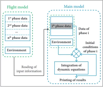
he creation of a light model in RTS comprises basically the selection of each model to be used, the deinition of a sequence of events, which establishes the several phases of the trajectory, and the deinition of the models that will be active in each phase. his process is illustrated in Fig. 3. Once the light model is ready, the integration of the trajectory equations can be performed by the main module, as shown in Fig. 4. he output results are the
several light parameters like position, velocity and acceleration of the vehicle, the forces and moments from propulsion and aerodynamics etc.
he architecture of RTS was deined to fulill the requirement for flexibility. During the integration of the trajectory, the successive calls to the models comprised in the light model obey a predeined sequential order, as shown in Fig. 5. his order follows a logical calculation sequence of the several light parameters of the simulation, in a way that the information needed by a model has already been calculated by the models executed previously.
The first executed models belong to the environment category and compute the gravitational, atmospheric and wind properties at the vehicle position. Next, the subsystems
Figure 3. Flight model creation in RTS.
Flight model Library
Enviroment model Vehicle/Trajectory model
Environment Environment 1 Environment 3 1st phase data
2nd phase data
Dynamics1 Subsystem 1 Subsystem 3 Auxiliary 2
... nth phase data
Event 1
Event 2 Event n–1 Dynamic models
– Dynamics 1 – Dynamics 2
Vehicle subsystems models – Subsystem 1
– Subsystem 2 – Subsystem 3
Auxiliary tools – Auxiliary 1 – Auxiliary 2
Environment models – Environment 1 – Environment 2 – Environment 3
Se
quen
ce o
f e
ven
ts
State variables at time t
State variables at time t+δt Earth
Atmosphere
Wind
Discrete control
Control
Mass properties
Propulsion
Aerodynamics
Auxiliary
Dynamics
∫
Main model
Flight model
Reading of input information
1st phase data
2nd phase data
...
nth phase data
Environment
Environment
Printing of results Integration of dynamic equations
Initial conditions
of phase i Data of phase i ith phase data
Figure 4. Trajectory integration in RTS.
models are called, and several vehicle properties are calculated, including control actions and eforts, like nozzle delection, mass properties, and also aerodynamic and propulsion parameters and eforts. Next, the auxiliary tools can be used to calculate the parameters not comprised by the previous models, like the vehicle position with respect to a radar, for instance. Finally, with all eforts that act on the vehicle, the dynamic model is executed, and the state variables that describe the vehicle motion are integrated. If a discrete control model is included, it is executed outside the integration loop. Except for the dynamic model, more than one model of a speciic category can be executed. his is useful when, for example, two kinds of controllers or propulsive systems are active at the same time.
he integration process of the state variables is performed
by a MATLAB® build-in function, the ode45. his is an initial
value problem solver based on an explicit Runge-Kutta (4,5) formula. It is a one-step solver, meaning that the solution at a time instant depends only on the solution at the immediately preceding instant. he time step, represented by δt in Fig. 5, varies according to the solver capability to find a solution that satisies the error tolerance criteria, and, for the present application, it generally lies between 10-3 and 100.
he architecture of RTS enables the light simulation of a variety of launch vehicles, since the appropriate models are present in the library. his lexibility is enhanced with the possibility of the user to add models to the library in a relatively easy way. A key-characteristic of RTS that enables the addition of new models is that all parameters computed during a time step of the integration are stored in a common structure where the access to the contents of the variables is made by their name. By using this structure as input and output arguments to all models, including those added by the user, it permits the models to access all the needed variables and also to store the information calculated so far, making this information available to all other models executed later. his characteristic is illustrated in Fig. 6, where a nozzle delection signal, βpitch , is calculated as a function of the vehicle attitude, θ, and angular speed, q, and
is stored in the same structure containing these parameters. In the igure, kθ and kq are constants of the controller.
RESULTS AND DISCUSSION
In order to verify the results of RTS, two diferent light scenarios were simulated. he results were compared with two diferent simulation tools available at IAE. he simulations were performed
in an Intel® Core 2 Quad 2.66 GHz, with 1.94 GB of RAM.
he irst scenario was the simulation of VSB-30, an unguided and aerodynamically stabilized Brazilian sounding rocket composed by two solid propellant stages and a payload. he vehicle is shown in Fig. 7. Launched from rail, it has the capacity of boosting a payload of around 350 kg to an altitude of 300 km (Garcia et al., 2011). he results of RTS were compared with those obtained with the tool Rocket Simulation (ROSI), a six degrees-of-freedom simulator used for light simulation of Brazilian rockets and already validated by actual light data. For this scenario, ROSI runtime was about 1 s and RTS runtime was about 59 s.
Figure 8 shows the altitude of the vehicle as a function of ground range. It can be seen the good agreement between the two simulators. he increasing diference that appears ater approximately 80 s of light is the result of a minor diference in the thrust correction method with altitude used in the two simulations. he results of light speed have also a good agreement, as it can be seen in Fig. 9. In this case, the diference that appears at the end of the trajectory is due to the fact that ROSI simulates the payload reentry considering the drag force, while RTS considers a free light during reentry. he diference in the results of altitude and speed can be better observed in Fig. 10, that shows this diference in relative terms.
One last result about VSB-30 concerns the roll speed. Figure 11 shows ROSI and RTS results, along with an actual light data. It can be seen that ROSI and RTS difer ater approximately 25 s of flight. This discrepancy is due to a simplification adopted in ROSI that does not consider the moment caused
Structure Structure
Control model
βpitch = kθθ + kqq
βpitch θ
θ q
q
Figure 8. Altitude versus ground range of VSB-30.
Figure 10. Altitude and light speed relative error between
RTS and ROSI.
Figure 9. Flight speed versus time of VSB-30.
Figure 11. Roll speed of VSB-30.
Figure 12. Comparison of roll moment due to aerodynamic
and inertia variation effects.
300
250
100
100 50
50 0
0 200
200 150
150
Ground range (km)
Al
ti
tu
d
e (
k
m)
ROSI RTS
5 0
1 0 0 2 0 0 3 0 0 4 0 0 5 0 0 6 0 0 0
0 -5 0 -1 0 0 -1 5 0
Time(s) 6 0
1 0 0 2 0 0 3 0 0 4 0 0 5 0 0 6 0 0 4 0
0 2 0
0 -2 0
Time(s)
A
ltit
u
d
e er
ro
r
(%)
Sp
ee
d
e
rr
or
(%)
2500
2000
1500
1000
500
0
0 100 200 300 400 500 600
F
lig
h
t s
p
ee
d (m/s)
Time (s)
ROSI RTS
Time (s)
ROSI RTS Actual
0 -200
200 -600 1000 1400
60 80
20 40
R
o
ll s
p
ee
d (d
eg/s)
Time (s)
Aerodynamic Inertia variation
R
o
ll mo
me
n
t (N
m)
0 0 20 40 60 80
10 20 30 40
by changes in the vehicle inertia. However, for rockets that
reach high roll speed, like VSB-30, this moment cannot be neglected, as conirmed by the actual light data presented in the igure. Is this case, this moment has the same order of magnitude than the aerodynamic moment, shown in Fig. 12.
he second scenario consisted of the VLM-1 simulation, the Brazilian microsatellite launcher, shown in Fig 13. VLM-1 is composed by three solid propellant stages (Agência Espacial Brasileira, 2012). he irst and second stages are controlled by gimbaled nozzles, while the third one has no control system. he results of RTS are compared with those obtained
with ASTOS®, a commercial simulation and optimization tool.
ASTOS® performs a simulation considering three
degrees-of-freedom of translation, while the vehicle rotation is considered
to happen ideally. For this scenario, ASTOS® runtime was
about 9 s and RTS runtime was about 180 s.
The trajectory of the mission SHEFEX III, a German suborbital mission, was simulated here. Figures 14 and 15 show the vehicle position and speed. It can be seen that the results
of RTS and ASTOS® are in good agreement. Figure 16 shows
the relative diference between the two simulations.
Despite the good agreement of the results just presented, the diference between a three and a six degrees-of-freedom simulation can be better observed when the parameters analyzed are directly related to the vehicle rotation dynamics.
Figure 14. Altitude versus ground range of VLM-1.
Figure 15. Flight speed of VLM-1.
Figure 17. Pitch angle of VLM-1.
Figure 16. Altitude and light speed relative error between
RTS and ASTOS®.
an ideal rotation dynamics, the vehicle attitude at each instant will be exactly equal to the provided reference attitude. In RTS, on the other hand, the vehicle control system is responsible to drive the attitude to the reference trajectory. Figure 17 shows the pitch angle of the vehicle during the light. Overall, both
ASTOS® and RTS pitch attitude are in good agreement, meaning
that the control system model used in RTS is adequate to follow the reference for the pitch angle. However, some diferences can be seen in speciic portions of the trajectory.
Figure 13. VLM-1 vehicle, adapted from Agência Espacial
Brasileira (2012).
250
200
150
100
50
0
0 200 400 600 800 1000 1200 1400 1600
Al
ti
tu
d
e (k
m)
Ground range (km)
A STOS RTS
7000
6000
5000
4000
3000
2000
1000
0
0 100 200 300 400 500 ASTOS RTS
F
li
g
h
t s
p
ee
d (m/
s)
Time (m/s)
0
- 2 0
- 4 0
- 6 0
- 8 0
- 1 0 0
- 1 2 0
0 1 0 0 2 0 0 3 0 0 4 0 0 5 0 0
Time (s)
P
it
ch a
n
g
le (d
eg)
ASTOS RTS Time(s)
0.2
100 200 300 400 500
0
0
100 200 300 400 500
0
-0.4 -0.2
-0.6 0.4 0.2
-0.2 0
-0.4
Time(s)
A
ltit
u
d
e er
ro
r
(%)
Sp
ee
d
e
rr
or
(%)
Figure 18. Pitch angle of VLM-1 at the beginning of light.
1 0
-1 -2 -3 -4 -5 -6 -7 -8
0 2 4 6 8 10 12
Time (s)
P
it
ch a
n
g
le (d
eg)
ASTOS RTS
Figure 18 shows the pitch angle at the beginning of light. Due
to its ideal rotation dynamics when simulated with ASTOS®,
CONCLUSION
his paper presented the development of RTS, a simulation tool suited to investigate the light dynamics of launch vehicles. he tool was implemented considering requirements of lexibility, following a trend observed in research institutes and companies around the world. To fulil this requirement, a modular programming strategy was used successfully. he models present in the library of RTS and also the tool’s architecture have shown to be adequate to simulate the light of diferent types of launch vehicles.
he test cases presented have shown a good agreement of RTS with other tools already used to simulate the light dynamics
of launch vehicles. he diferences observed in the results of
RTS with respect to ROSI and ASTOS® were explained by the
diferences in the used models. Notably, results concerning the roll speed indicated that the simpliication adopted in ROSI, where the moment caused by the inertia variation is neglected, could compromise the simulation results.
ACKNOWLEDGEMENTS
he authors are thankful to INPE and IAE for the opportunity to develop this study.
REFERENCES
Agência Espacial Brasileira, 2012, “Programa Nacional de Atividades Espaciais, PNAE: 2012-2021”, Ministério da Ciência, Tecnologia e Inovação, Agência Espacial Brasileira, Brasília, Brazil.
Albertson, C., Tartabini, P.V. and Pamadi, B.N., 2012, “End-to-End Simulation of Launch Vehicle Trajectories Including Stage Separation Dynamics”, Proceedings of AIAA Atmospheric Flight Mechanics Conference, Minneapolis, USA.
Baldesi, G. and Toso, M., 2012, “European Space Agency’s Launcher Multibody Dynamics Simulator Used for System and Subsystem Level Analyses”, CEAS Space Journal, Vol. 3, No. 1-2, pp. 27-48. doi: 10.1007/s12567-011-0023-9
Betts, K.M., Rutherford, R.C., McDufie, J., Johnson, M.D., Jackson, M. and Hall, C., 2007, “Time Domain Simulation of the NASA Crew Launch Vehicle”, Proceedings of AIAA Modeling and Simulation Technologies Conference and Exhibit, Hilton Head, USA.
Cornelisse, J., Schöyer, H. and Wakker, K., 1979, “Rocket Propulsion and Spacelight Dynamics”, Pitman, London, United Kingdom.
Cremaschi, F., Huertas, I., Wiegand, A., Jung, W. and Scheuerplug, F., 2010, “6-Dof Trajectory Simulation and Optimization for Sounding Rockets”, Proceedings of International Conference on Astrodynamics Tools and Techniques, Madrid, Spain.
Falck, R. and Gefert, L., 2007, “Crew Exploration Vehicle Ascent Abort Trajectory Analysis and Optimization”, Proceedings of AIAA Guidance, Navigation and Control Conference and Exhibit, Hilton Head, USA.
Garcia, A., Yamanaka, S.S.C., Barbosa, A.N., Bizarria, F.C.P., Jung, W. and Scheuerplug, F., 2011, “VSB-30 Sounding Rocket:
History of Flight Performance”, Journal of Aerospace Technology and Management, Vol. 3, No. 3, pp. 325-330. doi: 10.5028/ jatm.2011.03032211
Greensite, A., 1967, “Short Period Dynamics”, NASA, Marshall Space Flight Center, Huntsville, USA.
Hughes, P.C., 2004, “Spacecraft Attitude Dynamics”, Dover, Mineola, USA.
Ippolito, C.A. and Pritchett, A.R., 2000, “Software Architecture for a Reconigurable Flight Simulator”, Proceedings of AIAA Modeling and Simulation Technologies Conference, Denver, USA.
Lu, P. and Rao, P.P., 2004, “An Integrated Approach for Entry Mission Design and Flight Simulations”, Proceedings of AIAA Aerospace Sciences Meeting and Exhibit, Reno, USA.
Mooij, E., 1997, “The Motion of a Vehicle in a Planetary Atmosphere”, Delft University of Technology, Faculty of Aerospace Engineering, Delft, The Netherlands.
Sarma, I., Prasad, U. and Vathsal, S., 1978, “Computer Simulation Methods for Launch Vehicle Mission and Control Problems”, Proceedings of the Indian Academy of Sciences Section C: Engineering Sciences, Vol. 1, No. 4, p. 423-440. doi: 10.1007/ BF02842910
Steele, M.J., Mollaghasemi, M., Rabadi, G. and Cates, G., 2002, “Generic Simulation Models of Reusable Launch Vehicles”, Proceedings of Winter Simulation Conference, San Diego, USA.