ABSTRACT: Design and development of gas turbine components are a complex multidisciplinary process. At the beginning of the power class deinition and engine coniguration it is necessary to conduct a market study. The results obtained are used in gas turbine thermodynamic cycle calculations and analysis in order to deine the gas turbine design point. Several possible design points are evaluated during this procedure. After this step, the gas turbine components are designed, including: compressor, combustion chamber and turbine. For industrial gas turbine purposes, it is common to use a free turbine after the gas generator, also commonly named power turbine. In this work, a power turbine was initially designed by meanline techniques, considering internal loss mechanisms, to obtain the main dimensions. The geometries of the components were generated in a 3-D environment to make possible the mesh generation, process to discretize the physical domain into a computational domain and use a 3-D Computational Fluid Dynamics tool. The results from the meanline approach and from the 3-D turbulent low numerical simulations were compared to verify the turbine operational conditions and its predictions at design and off-design conditions. The gas turbine under study is a project, derived from a low thrust turbojet previously developed by Instituto de Aeronáutica e Espaço. The power turbine project uses the same turbojet gas generator, already designed and currently under tests.
KEYWORDS: Turbine, Design, Analysis, Gas Turbine.
One-Stage Power Turbine Preliminary
Design and Analysis
Cleverson Bringhenti1, Jesuíno Takachi Tomita1, Fernando de Araújo Silva2, Helder Fernando de
França Mendes Carneiro2
INTRODUCTION
he Instituto de Aeronáutica e Espaço (IAE) is one of the Brazilian government institutes responsible for conducting research and development related to aerospace engineering. IAE has been developing in conjunction with TGM industry and Instituto Tecnológico de Aeronáutica (ITA) a gas turbine project able to be used in two types of applications: a turbojet — in thrust class of 5 kN, and a turboshat — in a shat power class of 1.2 MW for power generation application.
he aim is to develop a gas turbine in which the economic feasibility can be justiied by its diferent usages, since its two classes employ the same gas generator. he irst version of the designed turbojet is installed in a test facility at IAE and its test protocol is under progress. he turboshat class was studied ater the design of the turbojet engine version. he power turbine preliminary design (Silva, 2012) was inished, but improvements in the aerothermodynamics, heat transfer, stress and strain calculations of the components are being performed.
his work presents the design of the power turbine, its aerothermodynamics, which was performed using a reduced-order numerical design tool and Computational Fluid Dynamics (CFD) simulations to verify the results from the preliminary design made by Silva (2012), providing the data needed for structural and heat transfer analysis, to be done aterwards. An in-house code written in FORTRAN language (Silva, 2012) was used to supply input data for commercial turbomachinery design sotware AxSTREAM® and to determine a preliminary design of a free power turbine. With the use of AxSTREAM® software the turbine Nozzle Guide Vane (NGV) and rotor
1.Departamento de Ciência e Tecnologia Aeroespacial – Instituto Tecnológico de Aeronáutica – Departamento de Turbomáquinas – São José dos Campos/SP – Brazil.
2.Departamento de Ciência e Tecnologia Aeroespacial – Instituto de Aeronáutica e Espaço – Divisão de Sistemas Aeronáuticos – São José dos Campos/SP – Brazil.
Author for correspondence: Cleverson Bringhenti | Instituto Tecnológico de Aeronáutica – Departamento de Turbomáquinas | Praça Marechal Eduardo Gomes, 50
Vila das Acácias | CEP: 12.228-900 – São José dos Campos/SP – Brazil | Email: [email protected]
blades were generated by an airfoil stacking procedure and the 3-D geometry was obtained. his 3-D geometry was carefully treated to start the mesh generation process using the sotware ANSYS TurboGrid®. he CFD solver used in this work was the ANSYS CFX® v.13.
POWER TURBINE DESIGN
he preliminary design process was performed using two diferent meanline numerical tools. he irst is an in-house tool developed by (Silva, 2012) and the second one is commercial software called AxStream®. Meanline means that all fluid properties including the turbomachinery dimensions are calculated at mean blade height. his technique neglects the viscous efects that are accounted using loss modelling. here are several loss models, each one adequate for each case; therefore, there is no general loss model. he average values of all luid properties from hub-to-tip are very close to the values obtained at mean radius. hereby, the use of meanline technique is very interesting to obtain fast results and solutions for a irst turbomachinery design process.
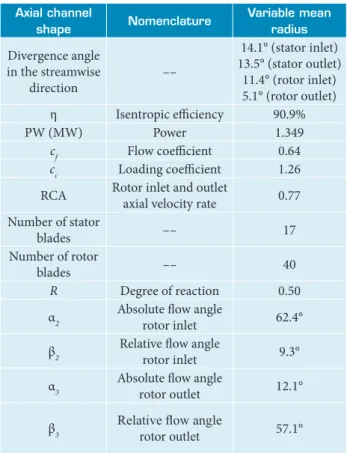
The main results from the meanline tool developed by (Silva, 2012) are presented in Table 1, in which the loss model developed by Kacker and Okapuu (1982) was used. he power turbine preliminary design was performed using AxSTREAM® sotware and it was conducted with the Craig and Cox (1970) loss model. Both loss models can be used at design and of-design conditions. For the power turbine studies, both loss models are adequate. For turbomachinery design several parameters must be varied and imposed by the designer during the preliminary sizing. Some design parameters and values were determined using an in-house code developed by Silva (2012) and the results used as an inlet data at the commercial sotware.
Along the years, several loss models were developed, for example: Ainley and Mathieson (1951), Denton (1978), Dunham and Smith (1968), Dunham and Came (1970), Dunham and Panton (1973), Rody et al. (1980) and Smith (1965). here are other models, but only the most commonly used were mentioned. In the present work, the loss models used are not described due to the high number of information, mainly about its calibrations, validation ranges, loss sources, constraints and so on. he reader that would like to understand the models in details it is highly recommended to search for the publication sources above mentioned.
he two-dimensional view of the power turbine stage, in the streamwise direction, calculated by AxSTREAM® making the use of the inlet data, calculated by the in-house code developed by Silva (2012), as presented in Table 1, is shown in Fig. 1a. he blue component is the stator row (or NGV) and the red component is the rotor row.
Axial channel
shape Nomenclature
Variable mean radius
Divergence angle in the streamwise
direction
––
14.1° (stator inlet) 13.5° (stator outlet)
11.4° (rotor inlet) 5.1° (rotor outlet)
η Isentropic eiciency 90.9%
PW (MW) Power 1.349
cf Flow coeicient 0.64
cc Loading coeicient 1.26
RCA Rotor inlet and outlet
axial velocity rate 0.77 Number of stator
blades –– 17
Number of rotor
blades –– 40
R Degree of reaction 0.50
α2 Absolute low angle
rotor inlet 62.4°
β2 Relative low angle
rotor inlet 9.3°
α3 Absolute low angle
rotor outlet 12.1°
β3 Relative low angle rotor outlet 57.1°
Table 1. Power turbine preliminary data.
Figure 1. Power turbine meridional view. (a) NGV row in blue and rotor row in red; (b) Different sections.
Section 2 Section 3 Section 1
(a)
THE 3-D TURBINE FLOW
CALCULATIONS
Since the aim of this study is to discuss the preliminary design results obtained previously Silva (2012), in this paper there are no discussions about numerical schemes, turbulence models, spatial and time marching methods, discretization issues and other topics around the CFD numerical implementations and its programming techniques. Certainly, all sotware and hardware used in numerical simulations demand high CPU time, currently called high performance computing (or HPC).
In this paper, the methods and models used are available in the open turbomachinery literature and additional details can be found in Craig and Cox (1970), Kacker and Okapuu (1982), Silva et al. (2011), Bringhenti et al. (2001), Tomita (2009), Silva and Tomita (2011) and Murari et al. (2011).
he turbine geometry calculated based on meanline technique was appropriately treated to generate its 3-D geometrical view making use of Computer-Aided Design (CAD) sotware. It is recognized that the CAD treatments, mesh generation processes and the low calculations using CFD technique are very time consuming processes.
he use of CFD techniques is very important during the turbomachinery design processes, because some low features cannot be visualized by the designer from meanline calculations, for example: boundary layer separation, high pressure gradients regions, shock wave position and expansion waves. hus, in order to calculate the 3-D low characteristics, the commercial CFD sotware ANSYS CFX® was used, with the calculations based on the Reynolds-Averaged Navier-Stokes equations (RANS). he turbulence efects were accounted using eddy viscosity turbulence model.
MESH GENERATION PROCESS
he mesh was generated using ANSYS TurboGrid® sotware. As this sotware is part of the environment, it also allows a direct link with other ANSYS® package sotware, such as CFX® for CFD calculation.
Different mesh configurations can be found in the TurboGrid® sotware. It is important to consider the control volume quality as its orthogonality, skew angles, aspect ratios, smoothing and others as presented in the references Silva et al. (2011), Silva and Tomita (2011) and Menter (1983).
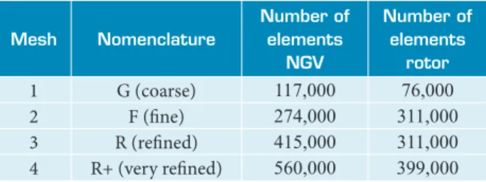
Four meshes with diferent reinements were generated to evaluate the mesh dependency for the particular turbine geometry studied. These meshes compromise hexahedral elements with the H/J/C/L conigurations to better accommodate the turbine geometry. At this point, it is important to mention that the y+ (position from blade surface at perpendicular direction) requirements must be considered, depending on the turbulence model that will be used to calculate the low eddy viscosity. he Reynolds number was deined relative to the chord, being 4.03 x 10⁵ at stator row and 2.68 x 10⁵ at rotor row.
The y+ value consists in determination of the distance between the irst centroid (or vertex) of the control volume at wall from the wall surface, ensuring that this distance is consistent with the turbulence model. he y+ is deined by the equation:
where:
ρ and μ: density and dynamic viscosity, respectively; Δy: y variation; τw: shear stress at wall.
Generally, for y+ ≤ 2, a very reined mesh must be generated. For y+ > 2, the CFD sotware determines the velocity ield using wall functions. It is recommended by CFD solver that the best practice to use the wall functions is for y+ values around 30 ≤ y+ ≤ 300. Diferent ranges can be found in the literature, but it is highly dependent on the wall functions implemented in each computational program.
Table 2 shows four mesh conigurations generated to perform the mesh dependency study. he meshes were generated and the luid mechanics equations were calculated until the point that there are no luid properties variation in the solution from CFD calculations. hese luid and low characteristics variations were considered in speciic streamwise locations (section 1, 2 and 3 as shown in Fig. 1b) and from blade hub-to-tip positions. For all cases, the numerical settings as spatial and time integration used in simulations are the same and the two-equation turbulence
Mesh Nomenclature
Number of elements
NGV
Number of elements
rotor
1 G (coarse) 117,000 76,000
2 F (ine) 274,000 311,000
3 R (reined) 415,000 311,000
4 R+ (very reined) 560,000 399,000
Table 2. Mesh conigurations data for each case considered.
(1)
y
+=
ρ
∆
y
μ
τ
wMesh G F R R+
η 89.0% 89.5% 90.2% 90.2%
m 7.182 7.704 7.684 7.677
TPR 1.98 1.97 1.97 1.97
y+ (ave.) 35 – 68 3 - 34 4 - 70 0.5 - 77
y+ (max.) 130 68 130 135
Time* 1,000 3,200 4,000 5,400
Table 3. CFD results for the four meshes.
*CPU time, in seconds per time integration iteration, in a computer with Microsoft Windows 7® 64bits operational system, 3.4 GHz i7 2600 processor with 8GB RAM memory available. m mass low rate; TPR: inlet and outlet total pressure rate.
.
.
model developed by Menter et al. (2004), called Shear-Stress Transport (SST), was used to calculate the low eddy viscosity. he details are described in the next section.
The Mach number, total pressure and static pressure were compared for all mesh configurations, and the values were calculated using mass averaging at each surface (section). Moreover, the isentropic efficiency, mass flow, expansion ratio and y+ values were monitored and analyzed for each mesh as shown in Table 3. The reference pressure value is 101,325 Pa.
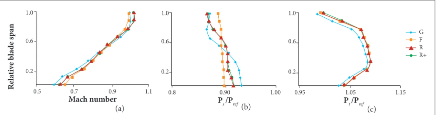
Figure 3. Distribution at section 2. (a) Mach number; (b) Static pressure (Ps); (c) Total pressure.
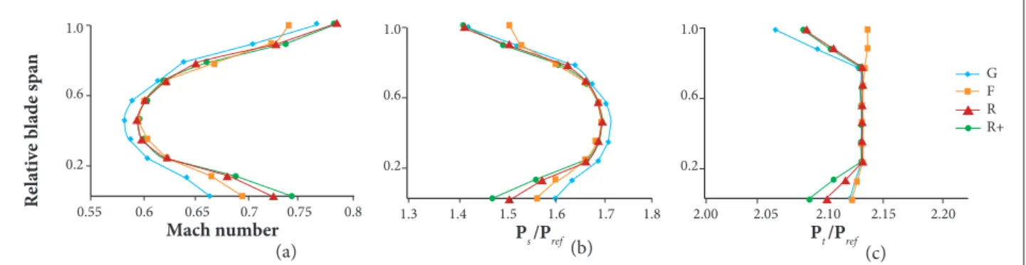
Figure 2. Distribution at section 1. (a) Mach number; (b) Static pressure (Ps); (c) Total pressure.
Figure 1b shows the stator and rotor section numbers used in this study, as well as the blade geometries.
Figures 2 to 4 show the low characteristics variations (Mach number, static and total pressures) for each mesh in diferent sections along the turbine blade span. he idea is to evaluate the CFD solutions for diferent mesh conigurations.
In Fig. 2, at section 1, it is possible to observe the impact of the velocity variations in diferent mesh conigurations and its inluence on Mach number and consequently on total pressure. he meshes R and R+ presented closely results. Note that, for 0 – 20% of blade span and for 80 – 100% of blade span, the results from diferent meshes present some interesting diferences. his is due to the inadequate mesh resolution close to the wall, where boundary-layer is very important and pronounced.
From Fig. 3, at section 2, the same behavior and explanation can be performed. he meshes R and R+ presented closely results including the mesh F. At this point, it is possible to mention that the mesh G is not recommended for the simulations like the ones used in this work.
In Fig. 4, at section 3, the mesh F presented small diferences in the solution when compared with the solutions from meshes R and R+. Again, the meshes R and R+ presented closely results including regions close to the turbine endwall and casing.
R
el
at
iv
e b
lad
e s
p
an
Mach number Ps /Pref Pt /Pref
1.0
0.6
0.2
0.55 0.6 0.65 0.7 0.75 0.8 1.3 1.4 1.5 1.6 1.7 1.8 2.00 2.05 2.10 2.15 2.20
1.0
0.6
0.2
1.0
0.6
0.2
G F R R+
R
el
at
iv
e b
lad
e s
p
an
Mach number Ps /Pref Pt /Pref
1.0
0.6
0.2
0.3 0.4 0.5 0.6 0.7 0.8 0.8 1.0 1.2 1.4 1.6 0.95 1.00 1.05 1.10 1.15
1.0
0.6
0.2
1.0
0.6
0.2
G F R R+
(a)
(a)
(b)
(b)
(c)
From these results it is possible to deine that the mesh R is more adequate for the numerical simulation of the turbine designed in this study. he mesh R+ is also an alternative, but it is more expensive (CPU time) than mesh R due to the high number of control volumes, becoming the mesh R the best compromise. Figure 5 shows the surface mesh characteristics at stator blade row. Regions close to the wall surfaces need more reinement, the smoothing at wall regions in the computational domain should be carefully built to ensure a good resolution of the boundary-layer and acceptable low characteristics resolution.
method for the mass terms, similar to the methodology proposed by Majumdar (1998).
For the discretization of convective terms from the Navier-Stokes equations, irst and second order upwind numerical schemes are available. he limiters proposed by Barth and Jesperson (1989) are used to control the numerical discretization order, mainly for discontinuously regions, and to avoid numerical instabilities in shock regions when upwind based methods are used. he difusion terms are discretized making the use of the shape functions. his methodology is usual in inite elements method (FEM) and has shown to be very robust for this purpose. he discretization model applied for the convective terms from Navier-Stokes equations was the second-order upwind scheme. To accelerate the numerical procedure, the anisotropic algebraic multigrid technique developed by Raw (1996) was used to avoid error propagation due to the irregular elements. Conservation requirements are imposed by the method during the coarsening process. CFX® has only implicit time-marching scheme for time integration. An automatic time-step calculation method was used to ensure good numerical stability during the simulation. Fast convergence with few numbers of iterations can be achieved using this implicit scheme. All simulations were done for steady-state regime.
To account the turbulence efects, the low eddy viscosity was calculated based on the two-equation Shear Stress Transport (SST) model Menter (1983). his model is adequate for the present analysis according to the recommendations and analysis from Menter et al. (2003, 2004), Denton (2010), and CFD Online (2011). he model uses the k-ω formulation at the internal region of the boundary layer and the k-ε model away from the wall. his control is determined using blending functions developed by Menter (1983).
he boundary-conditions were set at several surfaces as described:
Figure 5. Mesh at stator — pressure side surface.
Figure 4. Distribution at section 3.(a) Mach number; (b) Static pressure (Ps); (c) Total pressure.
NUMERICAL ISSUES AND
BOUNDARY CONDITIONS
he commercial sotware CFX® v.13 was used as a CFD solver to perform the low calculations based on the continuity, Navier-Stokes and energy equations. he compressible version of the solver was set-up. CFX® uses the coupling between the equations and the modiied Rhie and Chow (1982) discretization
R
el
at
iv
e b
lad
e s
p
an
Mach number Ps /Pref Pt /Pref
1.0
0.6
0.2
0.5 0.7 0.9 1.1 0.8 0.90 1.00 0.95 1.05 1.15
1.0
0.6
0.2
1.0
0.6
0.2
G F R R+
• At turbine NGV inlet: total pressure (Pt ) = 214,145 Pa, total temperature (Tt ) = 990.7 K, turbulent intensity = 5% and α = 19.18° (absolute low angle);
• At turbine rotor outlet: static pressure (Ps) = 89,891 Pa;
• Rotational speed = 27,920 rpm;
• Periodicity: blade-to-blade;
• At walls: no-slip condition;
• Inter-rows: mixing-plane approach.
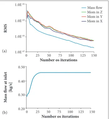
he solution from CFD solver was monitored by convergence criteria based on the residue decayment, number of iterations and mass-flow variations (if no changes in the mass-flow was detected, the solution can be considered achieved; this is common in the turbomachinery CFD applications).
Figure 6a shows the residual decayment of the continuity and momentum equations monitored during numerical iterations. he mass-low at turbine inlet was monitored during numerical iterations. Figure 6b shows the mass-low behavior during the numerical simulation. With 150 iterations the solution was considered achieved. An important numerical issue to mention is the very efective initial condition, also called initialization process used in the CFX® solver, in which, before the irst iteration, the solver estimates a good distribution of pressure, temperature and velocity ields along the turbine streamwise and blade span directions, to guarantee a good initial condition.
DESIGN-POINT ANALYSIS
At design-point condition, the turbine lowield was calculated using CFD technique and each blade row (NGV and rotor) was analysed separately. he low characteristics in important and/or critical regions were studied, as near to hub and tip zones, as well as the average values for some parameters at stage inlet and outlet sections. he static pressure distribution along each blade proile is plotted against its chord to evaluate the behavior of the low along the blade pressure and suction sides. he blade proile is a multi-circular arc (MCA).
he NGV Mach number and entropy contours for 20, 50 and 80% spanwise are shown in Figs. 7 to 9. It is important to mention that the scales considered in each igure are not held constant; this was done for better visualization.
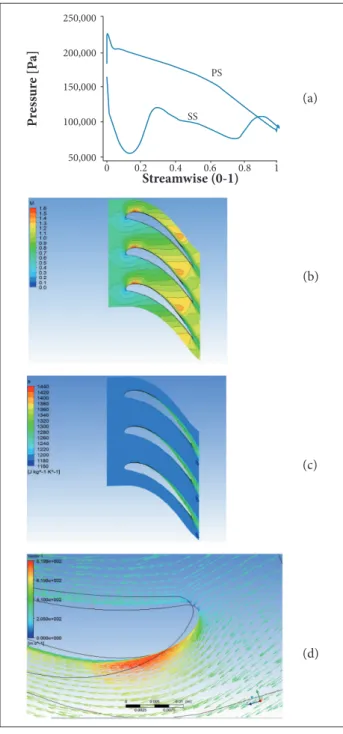
From Fig 7, it is possible to observe high low acceleration from NGV leading-to-trailing edge, but at 68% of the blade chord a sudden increase in static pressure is observed, causing low deceleration. he result is an increase in the entropy.
Figure 8 show the same analysis, but for 50% of the NGV blade span. Note that, at suction side, there are quite diferences in static pressure values when compared with the 20% of the NGV spanwise. his diference is because the low velocities are higher in regions close to the NGV hub. he degree of low deceleration at 50% of the NGV spanwise is lower when compared with 20% of the NGV spanwise. Hence, the internal losses are lower and, consequently, the entropy generation is decreased too.
Figure 9 show the results for 80% of NGV spanwise. Comparing the results of static pressure for diferent NGV blade span, it is possible to observe that the low acceleration region, close to the blade leading edge, at blade suction side, changes from around 12 to 18% of the blade chord. he blade angles and thickness chord ratio distributions are responsible for these variations.
Figure 9b shows small Mach number values when compared with Fig. 8b. his is a common low behavior along the NGV spanwise. he entropy generation are indications that some improvements in the blade design can be necessary to improve the low characteristics through the NGV channel.
For the blade pressure side, the results show a satisfactory pressure variation. At suction side, close to the hub, there is a supersonic bubble, covering the full low passage. Except for this bubble inluence, the results are in agreement with the prediction (Silva et al., 2012). Figure 10a provides a visualization of the velocity vectors related with the low acceleration at suction side at 20% of the NGV spanwise.
Figure 6. Numerical procedure. (a) History: continuity and momentum equations; (b) Turbine mass low variation.
RMS
M
ass fl
o
w a
t in
le
t
[kg/s]
Number os iterations Number os iterations
Mass flow Mom in Z Mom in Y Mom in X
0
0.20 0.30 0.40 0.50 1.0E-07 1.0E-05 1.0E-03 1.0E-01
25 50 75 100 125 150
0 25 50 75 100 125 150
(a)
Figure 7. NGV spanwise - 20%. (a) Static pressure variation along the blade chord; (b) Mach number contours; (c ) Entropy contours; (d) Velocity vector.
Figure 8. NGV spanwise - 50%. (a) Static pressure variation along the blade chord; (b) Mach number contours; (c ) Entropy contours.
he total pressure and Mach number distributions, in a midplane between blades of the same row, are shown in Figs. 10b and 10c. In these igures, it is possible to observe the radial variation of the low velocity and the high velocity region at NGV hub close to the trailing edge. he gas expansion is observed from the total pressure decreasing along the NGV blade chord.
he result also indicates that higher velocities at trailing edge, near to the hub, increase the internal losses due to the association with skin friction.
The total pressure distribution shows the influence of boundary-layer in the turbine hub and casing walls. he total pressure, Mach number and entropy distributions are shown at stator inlet and outlet sections (Figs. 11 to 13).
he inluence of boundary-layer should be carefully analyzed during the turbomachinery design process. Depending on the boundary-layer thickness, the inluence on the velocity ield is expressive, because an increase in velocity changes all low properties distributions and generates more internal losses, degrading the machine eiciency. he variation of the velocity along the streamwise direction is important due to the inluence on the gas expansion process related with the density variation.
Streamwise (0-1)
P
ress
ur
e [P
a]
250,000
200,000
150,000
100,000
50,000 0
PS
SS
0.2 0.4 0.6 0.8 1
Streamwise (0-1)
P
ress
ur
e [P
a] 200,000
150,000
100,000
0
PS
SS
0.2 0.4 0.6 0.8 1
(a)
(b)
(c) (b)
(a)
Figure 12. NGV outlet. (a) Total pressure contours; (b) Mach number contours.
Figure 10. NGV — blade-to-blade midplane. (a) Total pressure distribution contours; (b) Mach number contours.
Figure 11. NGV inlet. (a) Total pressure contours; (b) Mach number contours.
Figure 13. Entropy contours. (a) Stator inlet; (b) Stator inlet.
Figure 9. NGV spanwise - 80%. (a) Static pressure variation along the blade chord; (b) Mach number contours; (c ) Entropy contours.
Streamwise (0-1)
P
ress
ur
e [P
a] 200,000
150,000
100,000
0
PS
SS
0.2 0.4 0.6 0.8 1
(a)
(a) (b) (c)
(a) (a)
(a)
(b) (b)
Entropy generation sources are generated at walls, due to the low viscous efects and high velocities that are found in the blade-to-blade passage area; the velocity increases because the blade passage area is a convergent nozzle and high low delections are needed to improve the energy transfer. Moreover, diferent outlet blade angles and blade thickness distributions have strong inluence on the energy transfer process. he losses are associated with the low velocities and their growth is proportional to the velocity magnitude squared. As aforementioned, at the NGV domain, the low has higher velocities close to the hub regions and its losses can be observed in Fig. 13b, in which high entropy generation can be observed.
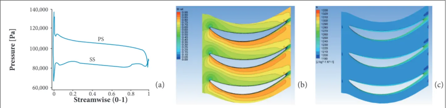
he same analysis was performed for rotor blade row as presented in the Figs. 14 to 16. he static pressure distribution along the blade chord at suction and pressure sides, Mach number and entropy contours are presented. he same spanwise percentages were used: 20, 50 and 80%. Figure 14a shows a good variation of static pressure at blade surfaces for 20% of the rotor spanwise.
It is possible to observe that the Mach number is lower than unity and the turbine is unchoked at the design-point. his is a preliminary design strategy to maintain a certain design lexibility during the preliminary analysis. Sometimes,
to obtain more power or pressure ratio, it is necessary to handle some possibilities. Hence, it is recommended that the design parameters not start with the limit values. Unlike NGV, at rotor hub, the velocity magnitude is lower than rotor tip values due to the tip speed. Figure 14b shows a good Mach number behavior of the low along the rotor passage. Figure 14c shows good characteristics around the entropy evaluation. here is no separation or serious problems close to the rotor trailing edge at 20% of rotor spanwise.
Figure 15 present the results for 50% of rotor spanwise. he low velocity across the rotor passage for this position is greater than 20% of rotor spanwise. Mach number reaches the unity. At this position the low is choked and a high energy transfer from luid to rotor is achieved.
hough the value of Mach number for 50% of rotor spanwise reaches the unity, the behavior of the low for this blade position is acceptable. he entropy increases only at rotor trailing edge. his is normal condition due to the low mixture in this region. he characteristic of the static pressure at 80% of the rotor spanwise is also acceptable, as shown in Fig. 16a. High Mach number can be observed at 80% of the rotor spanwise; this is due to the high tip speed values at this position, and supersonic
Figure 14. (a) Static pressure variation at 20% of the rotor spanwise; (b) Mach number contours at 20% of the rotor spanwise; (c) Entropy contours at 20% of rotor blade span.
Figure 15. (a) Static pressure variation at 50% of the rotor spanwise; (b) Mach number contours at 50% of the rotor spanwise; (c) Entropy contours at 50% of rotor blade span.
Streamwise (0-1)
P
ress
ur
e [P
a] 120,000
140,000
100,000
60,000 0
PS
SS
0.2 0.4 0.6 0.8 1
80,000
Streamwise (0-1)
P
ress
ur
e [P
a]
120,000 160,000
100,000
0
PS
SS
0.2 0.4 0.6 0.8 1
140,000
80,000
(a)
(a)
(b)
(b)
(c)
low can be reached as presented in Fig. 16b. In the present work, the tip Mach number reached the value of 1.2.
Some geometrical modiications at rotor blade in the suction side, around at 80% of rotor spanwise, can be necessary to improve the low characteristics in this region. he wake formation can be minimized changing the blade outlet angle and its thickness.
he entropy contours veriied in Fig. 16c is due to the mixing region. In general, the results from CFD simulations at 80% of the rotor spanwise are acceptable.
For the suction side, as at stator, the results show satisfactory behavior for the low property distributions. At rotor, there is a larger diference in low behavior between the three radial positions, as shown in Figs. 14 to 16. Near the hub, the low is almost subsonic and the parameter variations are sotly and small. his is a consequence of the use of low degree of reaction at this region.
Considering the analysis at hub, the low properties increase along the surface, becoming very smooth until approximately 60% of the chord, where it starts to sufer inluence from the suction side, as also occurs at NGV row. However, for the rotor, this variation increases until the trailing edge, what is a consequence of the smaller blade-to-blade passage due to the higher number of blades. he highest Mach number value, approximately 1.0, is obtained close to the tip. All these results are in agreement with the prediction described by Silva (2012).
At blade suction side, mainly close to the tip, low properties present great variation until the throat region (approximately 60% of the chord). At this point, the low properties start to oscillate, with a sequence of deceleration, acceleration and deceleration again, as can be seen in Figs. 16a and 16b. he maximum Mach number found in both accelerations does not exceed 1.2. hese results are also in agreement with the predictions made by Silva (2012).
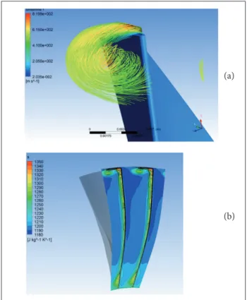
In Fig. 17a it is possible to see the influence of the tip clearance on the rotor flowfield. The radial variation of the pressure and the velocity in this location are high. The
clearance must be evaluated with a very careful process due to the high machine degradation related with the leakage flow. This leakage flow creates a secondary flow that interacts with the main flow. This mixing process generates high entropy and energy dissipation. Figure 17a shows the streamlines in this region. It is very common the structures formation, as scrapping vortex, that generally causes the drop in turbine efficiency.
Figure 17b shows the entropy contours at rotor row outlet with interesting vertical formations at rotor tip clearance region. In the same igure it is possible to observe the secondary low
Figure 16. (a) Static pressure variation at 80% of the rotor spanwise; (b) Mach number contours at 80% of the rotor spanwise; (c) Entropy contours at 80% of rotor blade span.
Figure 17. (a) Streamlines due to the rotor tip clearance; (b) Entropy contours at rotor outlet.
Streamwise (0-1)
P
ress
ur
e [P
a] 140,000
180,000
100,000
0
PS
SS
0.2 0.4 0.6 0.8 1
160,000
120,000
80,000
60,000
(c) (b)
(b)
(a)
Expansion rate Expansion rate
C
o
rr
ec
te
d mass fl
o
w [kg/s]
Is
en
tr
o
p
ic e
ffi
ci
enc
y [%]
P
o
w
er [MW
]
Expansion rate
Design point Design point CFD study
Preliminary study 1.21
7.2
6.4 6.8
6.0
1.43 1.65 1.87 2.09 2.31 1.21
92 2.0
1.6
1.2
0.8
0.4
0.0 90
88
86
84
1.43 1.65 1.87 2.09 2.31 1.21 1.43 1.65 1.87 2.09 2.31
Figure 18. (a)Correctedmass low; (b) Isentropic eficiency; (c) Power versus expansion rate. growing and acting in the main low, close to the hub, and
creating at rotor leading edge horseshoe vortex. he efects of tip clearance in axial low turbines that operate with high pressure ratios are severe for efficiency and gas expansion process. Several studies have been conducted to improve turbine performance decreasing the efects of tip clearance (Silva and Tomita, 2013; Ameri et al., 1998; Tallman, 2004; Lee and Choi, 2010; Tallman and Lakshminarayana, 2001; Azad et al., 2000; Bunker, 2014; Thulin et al., 1982; Sang and Byoung, 2008; Krishnababu et al., 2009).
he results shown in the previous igures present a satisfactory lowield within the axial low turbine domain. he power turbine stage performance can be evaluated through the parameters calculated from the CFD techniques, as shown in Table 4. For efficiency, power and mass flow rate in parenthesis, the AxSTREAM® predicted diferent values and are also shown the error.
Generally, 1-D methods use loss modeling developed for reduced-order design tools, as meanline. hese models should be calibrated for each design purpose. Some three-dimensional effects are not possible to account using 1-D tools, but, in general, the results agree for both techniques.
OFF-DESIGN POINT ANALYSIS
he of-design performance analysis was conducted only at the nominal speed of 27,920 rpm for comparison with the predicted results, varying the expansion ratio during the simulations. he results are presented in Fig 18 together with the preliminary study and its respective values.
Figure 18a shows the variation of mass-low with expansion ratio, in which the results from meanline and 3-D CFD are quite diferent. he CFD results show that the turbine choke condition is close to 6.85 kg/s of mass low. his value is lower than that the choke condition determined in the meanline tool. his is due to the boundary-layer growth along the turbine streamwise direction that is, generally, underestimated by reduced-order tools. With high boundary-layer thickness, the velocity in the main flow increases, causing choking conditions. Meanline tool generally uses very simple models to account the blockage along the streamwise directions and in some tools this value is estimated by the designer. he expansion ratio for both tools at design-point presented slightly values with a diference around 0.11. Based on the CFD results, the turbine is choked at design-point conditions. his is normal and is in agreement with turbine design methodology and means that high energy transfer occurs in the gas expansion process.
It is clear that a calibration of some coeicients used in the loss modeling should be adjusted to improve the turbine prediction for performance calculations. his is a very common action into the turbomachines design, in which, for several reasons, these
Parameter Value
η (%) 90.1 (90.9 – 0.8%)
PW (MW) 1.238 (1.349 – 8.2%)
m (kg/s) 7.717 (7.918 – 2.5%)
Inlet Outlet
Tt (K) 990 852
Ts (K) 923 815
Pt (Pa) 214,784 108,760
Ps (Pa) 162,619 90,724
Mrel –– 0.85
V (m/s) –– 482
β (°) –– 51.9
M 0.66 0.51
C (m/s) 390 273
α (°) 19.1 1.1
V: relative velocity; C: absolute velocity; M: Mach number.
Table 4. Turbine stage performance parameters.
(c) (b)
calibration issues are considered as proprietary information for each industry.
Figure 18b shows that the peak eiciency at design-point operation condition is slightly diferent for both tools with a diference of 0.6, in which the eiciency from CFD solution is lower. his is because the loss mechanisms determined by meanline are underpredicted. Generally, 3-D CFD considering viscous lows presents more accurate results due to the better representation of boundary-layers and luid friction. he eiciency determined by CFD tool is calculated based on mass-averaging process.
Figure 18c shows a good agreement between both numerical tools until the expansion rate of 1.98. he power determined by CFD tool is lower at design-point (around 160 kW lower than meanline tool). his can be explained due to the internal losses underpredicted by meanline tool. In general, all obtained results were well represented using the meanline tools, that are very fast to perform the calculations, comparing CPU time to calculate the 3-D turbulent low by CFD and simple correlations.
CONCLUSION
In this study an in-house code written in FORTRAN language Silva (2012) was used to supply input data for commercial turbomachinery design sotware AxSTREAM® and to determine a preliminary design of a free power turbine. With the use of AxSTREAM® sotware the turbine NGV and rotor blades were generated by an airfoil stacking procedure and the 3-D geometry was obtained. his 3-D geometry was carefully treated to start the mesh generation process using the sotware ANSYS TurboGrid®. Four meshes with different number of control volumes were generated to study the mesh dependence from CFD solver. he
CFD solver used in this work was the ANSYS CFX® v.13. Based on the mesh dependence study the mesh R was chosen to perform all other simulations of the turbine design-point and of-design point operational conditions.
he 3-D turbulent low within the turbine computational domain was performed using RANS method applied on the luid mechanics equations (continuity, momentum and energy). he numerical issues and boundary conditions were described in details. he simulation results from meanline and CFD tools were compared at design and of-design conditions. For both, the results are physically correct and are in agreement with the behavior of turbine lowield.
Improvements in blade proile can be performed to increase the turbine eiciency decreasing the internal losses as shown from CFD results. Future work can be developed to calibrate the loss model to be applied in this free power turbine design. he CFD tool can be used aiming at improvements in the loss modelling calibration process.
The numerical tools and the methodology used in the present work can be used for axial flow turbine design purposes.
ACKNOWLEDGEMENTS
Márcio Teixeira de Mendonça, TGM Turbinas, Fundação de Amparo à Pesquisa do Estado de São Paulo (FAPESP), Conselho Nacional de Desenvolvimento Cientíico e Tecnológico (CNPq), and Coordenação de Aperfeiçoamento de Pessoal de Nível Superior (CAPES) are acknowledged for their support to the research carried out at IAE and the Center for Reference on Gas Turbines of ITA.
REFERENCES
Ainley, D.G. and Mathieson, G.C.R., 1951, “A Method of Performance Estimation for Axial Flow Turbines”, British ARC, R&M 2974, Retrieved in May 7, 2015, from http://naca.central.cranield. ac.uk/reports/arc/rm/2974.pdf
Ameri, A.A., Steinthorsson, E., Rigby, D.L., 1998, “Effect of Squealer Tip on Rotor Heat Transfer and Eficiency”, ASME Journal of Turbomachinery, Vol. 120, No. 4, pp. 753-759. doi: 10.1115/1.2841786
Azad, G.S., Hart, J.-C., Teng, S., Boyle, R.J., 2000, “Heat Transfer and Pressure Distributions on a Gas Turbine Blade Tip”, Proceedings of the ASME Turbo Expo, Munich, Germany, GT2000-0194.
Barth, T.J. and Jesperson, D.C., 1989, “The Design and Application of Upwind Schemes on Unstructured Meshes”, AIAA Paper 89-0366.
Bringhenti, C., Barbosa, J.R. and Carneiro, H.F.F.M., 2001, “Variable Geometry Turbine Performance Maps for the Variable Geometry Gas Turbine”, Proceedings of the 16th Brazilian Congress of Mechanical Engineering, COBEM, Uberlândia, Brazil.
Bunker, R.S., 2014, “Turbine Heat Transfer and Cooling: an Overview”, Proceedings of the ASME Turbo Expo, San Antonio, USA, GT2013-94174.
Craig, H.R.M. and Cox, H.J.A., 1970, “Performance Estimation of Axial Flow Turbines”, Proceedings of the Institution of Mechanical Engineers, Vol. 185, No. 1, pp. 407-424. doi: 10.1243/PIME_ PROC_1970_185_048_02
Denton, J.D., 1978, “Throughlow Calculations for Transonic Axial Flow Turbines”, ASME, Journal of Engineering for Gas Turbines and Power, Vol. 100, No. 2, pp. 212-218. doi: 10.1115/1.3446336
Denton, J.D., 2010, “Some Limitations of Turbomachinery CFD”, Proceedings of the ASME Turbo Expo 2010, Glasgow, Scotland, GT2010-22540.
Dunham, J. and Came, P.M., 1970, “Improvement to the Ainley/ Mathieson Method of Turbine Performance Prediction”, ASME, Journal of Engineering for Gas Turbines and Power, Vol. 92, No. 3, pp. 252-256. doi:10.1115/1.3445349
Dunham, J. and Panton, J., 1973, “Experiments on the Design of a Small Axial Turbine”, IMEch Conference Publication, No. 3, pp. 56-65.
Dunham, J. and Smith, D.J.L., 1968, “Some Aerodynamic Aspect of Turbine Design”, Proceedings of AGARD Conference, Advanced Components for Turbojet Engines, AGARD CP 34, Part 2, pp. 21.1 – 21.15.
Kacker, S.C. and Okapuu U., 1982, “A Mean Line Prediction Method for Axial Flow Turbine Eficiency”, ASME, Journal of Engineering for Gas Turbines and Power, Vol. 104, No. 1, pp. 111-119. doi: 10.1115/1.3227240
Krishnababu, S.K., Newton, P.J., Dawes, W.N., Lock, G.D., Hodson, H.P., Hannis, J. and Whitney, C., 2009, “Aerothermal Investigations of Tip Leakage Flow in Axial Flow Turbines - Part I: Effect of Tip Geometry and Tip Clearance Gap”, Journal of Turbomachinery, Vol. 131, No. 1, pp. 011006-1-011006-14. doi: 10.1115/1.2950068
Lee, S.W. and Choi, M.Y., 2010, “Tip Gap Height Effects on the Aerodynamic Performance of a Cavity Squealer Tip in a Turbine Cascade in Comparison with Plane Tip Results: Part 2 - Aerodynamic Losses”, Experiments in Fluids, Vol. 49, No. 3, pp. 713-723. doi: 10.1007/s00348-010-0849-5
Majumdar, S.R., 1998, “Under Relaxation on Momentum Interpolation for Calculation of Flow with Nonstagarred Grids”, Numerical Heat Transfer, Vol. 13, pp. 125-132.
Menter, F.R., 1983, “Zonal Two-Equation k-ω Turbulence Model for Aerodynamic Flows”, AIAA Paper, Washington, USA.
Menter F.R., Kuntz, M. and Langtry, R., 2003, “Ten Years of Industrial Experience with the SST Turbulence Model”, Proceedings of the 4th International Symposium on Turbulence, Heat and Mass Transfer, Antalya, Turkey.
Menter, F.R., Langtry, R. and Hansen, T., 2004, “CFD Simulation of Turbomachinery Flows - Veriication, Validation and Modeling”, Proceedings of the European Congress of Computational Methods in Applied Sciences and Engineering, Jyvaskyla, Finland.
Murari, S., Sathish, S., Shraman, G. and Liu, J.S., 2011, “CFD Aerodynamic Performance Validation of a Two-Stage High Pressure Turbine”, Proceedings of the ASME Turbo Expo 2011, Vancouver, Canada, GT2011-45569.
Raw, M.J., 1996, “Robustness of Coupled Algebric Multigrid for the Navier-Stokes Equations”, AIAA Paper 96-0297.
Rhie, C.M. and Chow, W.L., 1982, “A Numerical Study of the Turbulent Flow Past an Isolated Airfoil with the Trailing Edge Separation”, AIAA Paper 82-0998.
Rody, F., Varetti, M. and Tomat, R., 1980, “Low Pressure Turbine Testing”, AGARD CP 293, pp. 30.1-30.13.
Sang, W.L. and Byoung, J.C., 2008, “Effects of Squealer Rim Height on Aerodynamic Losses Downstream of a High-Turning Turbine Rotor Blade”, Experimental Thermal and Fluid Science, Vol. 32, No. 8, pp. 1440-1447.
Silva F. A., 2012, “Preliminary Design and Analysis of a Axial Turbine Stage for Conversion of a Turbojet to Turboshaft” (in Portuguese), Master Thesis, Instituto Tecnológico de Aeronáutica, São José dos Campos, Brazil, 183p.
Silva, F.A., Bringhenti, C., Carneiro, H.F.F.M., 2012, “Power Turbine Preliminary Design Used to Convert a Small Turbojet to Turboshaft”, Proceedings of the CONEM 2012, VII Congresso Nacional de Engenharia Mecânica, São Luís, Brazil.
Silva, D.T. and Tomita, J.T., 2011, “Axial Turbomachinery Flow Simulations with Different Turbulence Models”, Proceedings of the 21st Brazilian Congress of Mechanical Engineering, Natal, Brazil.
Silva, L.M. and Tomita, J.T., 2013, “A Study of the Heat Transfer in a Winglet and Squealer Rotor Tip Conigurations for a Non-Cooled HPT Blade Based on CFD Calculations”, ASME TurboExpo, GT2013-95164.
Silva, L.M., Tomita, J.T. and Barbosa, J.R., 2011, “A Study of the Inluence of the Tip-Clearance of an Axial Turbine on the Tip-Leakage Flow using CFD Techniques”, Proceedings of the 21st Brazilian Congress of Mechanical Engineering, Natal, Brazil.
Smith, S.F., 1965, “A Simple Correlation of Turbine Eficiency”, Journal of Royal Aeronautical Society, Vol. 69, pp. 467-470.
Tallman, J.A.A., 2004, “Computational Study of Tip Desensitization in Axial Flow Turbines Part 2: Turbine Rotor Simulations with Modiied Tip Shapes”, Proceedings of the ASME Turbo Expo, Vienna, Austria, GT2004-53919.
Tallman, J.A.A. and Lakshminarayana, B., 2001, “Methods for Desensitizing Tip Clearance Effects in Turbines”, Proceedings of the ASME Turbo Expo, New Orleans, USA, GT2001-0486.
Thulin, R.D., Howe, D.C. and Singer, I.D., 1982, “Energy Eficient Engine - High-Pressure Turbine Detailed Design Report” (NASA CR-165608), Cleveland, USA.