ABSTRACT: The inluence of variable-sweep wing on the aircraft’s radar cross section (RCS) characteristics has been studied to reduce the aircraft’s RCS as well as its detection probability by the hostile radar. With the help of CATIA, a 3-D digital model of the variable-sweep wing aircraft is built to generate a series of digital grids. Using MATLAB, a numerical simulation on the RCS of variable-sweep wing aircraft is conducted based on physical optics (PO) method and equivalent currents method (ECM). The results of mathematical statistics and comparative analysis show that: (i) the RCS peak value in the head direction of the aircraft decreases non-linearly with the sweep angle of the wing’s leading edge; (ii) the azimuth angle corresponding to one of the peak values of the aircraft’s RCS is equal to the leading edge’s sweep angle; (iii) when the leading edge’s sweep angle is 33°, the arithmetic average value of the RCS values in the head direction of the aircraft is 0.644% of the average value when the sweep angle is 0°; (iv) the larger the sweep angle is, the lower the probability that the aircraft is detected.
KEYWORDS: Aircraft conceptual design, Radar cross section, Variable-sweep wing, Stealth performance, Numerical simulation.
Numerical Simulation on the Radar Cross
Section of Variable-Sweep Wing Aircraft
Shichun Chen1, Kuizhi Yue1,2, Bing Hu1, Rui Guo1
INTRODUCTION
Stealth aircraft or low-observability aircraft is a very important developing direction for modern combat aircrat. In view of this trend, the main military powers all over the world are conducting studies on the stealth aircrat’s designing, manufacturing, arming and application. Typical stealth aircrat developed by the U.S. include F-22, B-2, F-35, X-45 and X-47 (Nangia and Palmer, 2005; Vogel, 2005). hese aircrat have become or will become the backbone elements of the U.S. Air Force and U.S. Navy. Russia is also developing its Su-47, MG-1.44, T-50, and other stealth combat aircrat, which are likely to become the future main force of the Russia Air Force. China’s aviation industry has also taken part in this competition and has achieved considerable success in developing its stealth combat aircrat. Variable-sweep wing aircrat have a glorious history. Classical aircrat such as the U.S. F-14, F-111, have participated in many wars. hey are once the real backbone elements of the U.S. Navy and Air Force. In Russia, MG-23, Su-24, Tu-160, and other aircrat are still performing a variety of combat missions. his paper conducts feasibility studies on the stealth design of the variable-sweep wing aircrat. The RCS features are explored to provide reference and theoretical support for the aircrat’s conceptual design and stealth optimization and thus provide technical reserves for the development of new stealth aircrat.
Researchers have performed lots of work on designing stealth aircraft for many years and have achieved quite many results. The different shapes of the stealth aircraft, including the aircraft’s head, fuselage, wings, inlets and other strong scattering parts of electromagnetic waves, have been studied(Wood and Bauer, 2001). Stealth materials are
1.Beijing University of Aeronautics and Astronautics – School of Aeronautic Science and Engineering – Beijing 100191 – China. 2.Naval Aeronautical and Astronautical
University – Department of Airborne Vehicle Engineering – Yantai 264001 – China.
Author for correspondence: Yue Kuizhi | Beijing University of Aeronautics and Astronautics – School of Aeronautic Science and Engineering | Beijing 100191 – China Email: [email protected]
analyzed and the key technologies of radar stealth, infrared stealth, visible and acoustic stealth are explored as well. Moreover, multidisciplinary optimization algorithms on pneumaticity, stealth and structure are investigated. Bai and Liu (2007) have studied the parametric modeling approach for fuselage sections. Taking into account the aircraft’s stealth performance, their approach generates the body shape by adjusting the body parameters. Tom and Alfred (2010) have studied the relationship between the aircraft’s configuration and its stealth performance when the resistance is the lowest. In Bao and Wang (2012), the characteristic parameters of flying wing’s stealth performance and aerodynamic performance are investigated, and a wind tunnel test of the flying wing is conducted. Ji et al. (2009) have studied the impact of the relative bending of the vertically- and horizontally-bended inlet on the inlet’s microwave scattering characteristics. Huang and Liu (2008) have studied the microwave scattering characteristics of the aircraft’s surface cracks by RCS measuring. He et al. (2010) have studied the influence of inhomogeneous plasma on the attenuation of planar electromagnetic waves. Sun and Zhang (2008) have summarized the characteristics of F/A-22 and F-35 stealth fighter jets and have proposed a conceptual solution to reduce the antenna aperture size along with the antenna aperture characteristic signal, adopting the technology of low intercept probability. Lu and Wang (2009) have studied the infrared radiation model of the aircraft’s surface, analyzed the aircraft’s infrared characteristics, and summarized the infrared stealth reduction strategies. Hu and Yu (2011) have studied the applications of multidisciplinary optimization to aircraft’s conceptual design, where the aircraft’s aerodynamic performance, stealth performance, structure design, general layout and weight constraints are all taken into consideration. Generally speaking, a series of issues about the stealth aircrat have been studied deeply; however, there are few research reports about the inluence of angle changes of the variable-sweep wing aircrat on its stealth characteristics. he qualitative and quantitative relationship between the wing’s leading edge sweep angle of the variable-sweep wing aircrat and the aircrat’s stealth performance still remains unclear. his paper focuses on the stealth characteristics of the variable-sweep wing aircrat. Physical Optics (PO) method and the Equivalent Currents Method (ECM) are used. A numerical simulation is conducted to obtain an analytical report of the RCS characteristics, so as to provide reference for the designing of stealth aircrat.
THEORETICAL BASIS
he theoretical basis of this study consists of two parts: RCS prediction methods and radar detection probability model.
RCS PREDICTION METHODS
A series of numerical simulations of RCS characteristics of variable-sweep wing aircrat are conducted in this paper. Scattering surface elements are calculated using PO method. Edge difraction is calculated by ECM. In PO method, it is assumed that the surface current on the incident point of the wave is equal to the surface current when the incident wave is just on the tangency plane of the incident point.
he formula of PO method is as follows (Yue et al., 2014b):
where:
√σpo: RCS of a single surface element, in m2; n: outward
normal unit vector of the surface element; er: direction of electric field on the receiving antenna; hi: direction of the incident wave’s magnetic ield; “ . ” is the dot product and “×” is the cross product; j: imaginary unit, and j2 = 1; λ: incident wavelength, in m; r0 : reference point on the surface element; s: scattering wave’s direction; i : incident wave’s direction; p = n × (s – i); A: area of the surface element, in m2; L
m: magnitude and direction of the mth edge; k: wave number, 2π/λ; r
m: vector from the reference
point r0 to the midpoint of the mth edge.
he formula of ECM is as follows:
where:
t: mandatory edge unit vector’s direction; i: incident wave; E0i: strength of the incident electric ield; f and g: Yoie Roussef
(1)
(2)
(3)
ˆ
ˆ
ˆ
ˆ
ˆ
ˆ
difraction coeicients; s: scattering wave’s direction; Z0: wave impedance in vacuum; H0i: strength of the incident magnetic ield; rt: position vector of the middle of the edge; l: vector of the edge; θ: angle between i and t. Other symbols’ deinition can be found in Yue et al. (2014a, 2014c, 2014d, 2015).
he superposition formula of the RCS of variable-sweep wing aircrat is as follows:
coeicient in the receiver, in dB; L: total system losses, in dB; R: detection distance, in m; σφγβ: RCS of the aircrat when the azimuth angle is φ, the rolling angle is γ, and the pitching angle is β, in m2.
In order to demonstrate the inluence of the varying sweep angle on the detection probability, we choose a typical ground-to-air searching situation for simplicity. In this situation, the aircrat is assumed to ly right towards the searching radar, and only the pitching angle varies with the detection distance. he pitching angle of the incident wave relative to the aircrat can be calculated as follows:
he arithmetic average RCS of the aircrat is shown as follows:
he unit-conversion formula of the aircrat’s RCS is shown as follows:
where:
σ: RCS of the variable-sweep wing aircrat, in m2; σ
φ: RCS in m2 when the pitching angle of the incident wave is β and
the azimuth angle of the aircrat is φ; σn~N: average value of RCS when the pitching angle of the incident wave is β and the azimuth angle φ ranges from n to N; σdBm : RCS of the variable-sweep wing aircrat, in dBm2.
RADAR DETECTION PROBABILITY MODEL
he probability that the aircrat is detected by a pulse Doppler radar can be estimated as follows Yue et al. (2010):
where:
PDk: detection probability of the target; Δθα: horizontal width of the radar lobe, in degrees; fr: radar’s pulse repetition frequency (PRF), inHz; Ω: radar’s scanning angular velocity, indegrees/s; Pt: radar transmitting power, in Watts (W); G: antenna gain, in dB; E: pulse compression ratio of the pulse compression radar; kb: Boltzmann constant, and its value is 1.38x10⁻²³Ws/K; T
0: standard room temperature, and its value
is 290K; Bn: noise bandwidth in the receiver, in Hz; Fn: noise
where:
β: pitching angle of the incident wave relative to the aircrat, in degrees. β is negative when the incident wave is below the aircrat; βf: pitching angle of the aircrat relative to the ground, in degrees. It is negative when the aircrat’s nose is upward; hd: vertical distance between the aircrat and the sea level, in km; hm: vertical distance between the radar and the sea level, in km; Rd: radius of the Earth and it is 6,371 km in general.
ALGORITHM VERIFICATION IN MICROWAVE ANECHOIC CHAMBER
In order to verify the effectiveness of the numerical simulation method that combines the PO method and the ECM, we have conducted a verification experiment in a microwave anechoic chamber.
he experiment procedure is as follows:
• Use CATIA to build a 3-D digital model of the aircrat, as shown in Fig. 1a.
• Use a 3-D printer to make a 1:36 scaled wax model, as shown in Fig. 1b.
• Transform the wax model into a sand model cavity and caste aluminum in the sand mold cavity to get a 3-D model in the state of cast-aluminum model, as shown in Fig. 1c.
• Conduct the RCS measurement experiment on the cast-aluminum model in the microwave anechoic chamber, as shown in Fig. 1d.
(4)
(5)
(8)
(9)
(6)
(7)
σ
dBm2=
101
g
σ
2
β
Figure 3. CATIA model of variable-sweep wing aircraft.
Figure 4. Schematic diagram of wing leading edge’s sweep angle.
The initial conditions of numerical simulation are: the incident wave is at X band and of horizontal polarization. he pitching angle of the incident wave is 0°. he azimuth angle of the aircrat is between 0° ~ 180°. Use PO method and ECM to do the numerical simulation on the 3-D digital prototype shown in Fig. 1a, and the RCS characteristics curve can be obtained as shown in Fig. 2.
According to the similarity principle, the incident wavelength should be 0.83 mm when conducting the RCS measurement experiment in the microwave anechoic chamber. And the incident wave should also be of horizontal polarization. he measurement results are shown in Fig. 2.
From the comparison between the numerical simulation and experimental results, we can see that the two RCS characteristic curves basically match each other. Ater verifying the scientiic character and accuracy of the numerical simulation method, we can use this method to analyze the RCS characteristics of the aircrat.
NUMERICAL SIMULATION OF
AIRCRAFT’S RCS
Numerical simulation of aircrat’s RCS consists of four components: CATIA modeling of the variable-sweep wing aircrat, numerical simulation of the aircrat’s RCS, analysis of the impact of wing leading edge’s sweep angle on aircrat’s RCS, and the probability of being detected by a searching radar.
CATIA MODELING OF THE VARIABLE-SWEEP WING AIRCRAFT
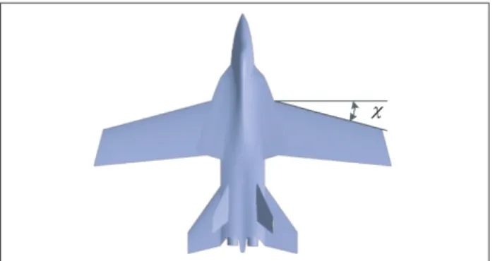
he variable-sweep wing aircrat scheme in this paper has adopted features as follows: single-seat, twin-engine, twin vertical tails extraversion, variable-sweep wing aerodynamic layout, the band edge of the wing and blended wing body. Double S-shaped bend inlets are adopted on both sides of the fuselage, and three bomb bays are buried into the fuselage. Figure 3 shows the layout of the aircrat.
The CATIA model of the variable-sweep wing aircraft uses parametric designing method to design the wing leading edge’s sweep angle, which is deined as χ (Fig. 4). Other basic parameters of the aircrat remain unchanged, in which the length of the aircrat is 22 m.
σ
/dB
m
2
φ/o
Electromagnetic testing Numerical simulation 30
20
10
-10
-20 0
0 40 80 120 160
Figure 2. Comparison of the aircraft’s RCS between
numerical simulation and experiment results.
Figure 1. Microwave chamber experiment. (a) 3-D digital model;
(b) Wax model; (c) Cast-aluminum model; (d) Microwave chamber. (a)
(c)
(b)
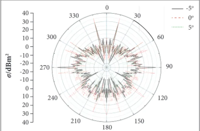
Figure 5. 3-D grids of aircraft when χ = 15°.
Figure 6. RCS characteristics of the aircraft when χ = 15°.
NUMERICAL SIMULATION OF THE AIRCRAFT’S RCS
CATIA is used in this study to establish a 3-D digital model for the variable-sweep wing aircrat. Analysis manager module is used to generate the 3-D grids (Fig. 5). Based on PO method and ECM, we import the aircrat 3-D grids to the RCS calculating program written in Matlab language. Under the conditions that the radar incident wave is at X band and of horizontal polarization, the pitching angle of the incident wave is –5°, 0° and +5°, and the azimuth angle of the aircrat is between 0° ~ 360°. In this section, we conduct a numerical simulation of the RCS of the variable-sweep wing aircrat and then obtain the RCS characteristic curve of the variable-sweep wing aircrat when χ = 15° (Fig. 6).
In the polar coordinates of the aircrat’s RCS characteristic, the azimuth angle 0° corresponds to the head direction of the aircrat and the azimuth angle 180° corresponds to the tail direction of the aircrat. And when the azimuth angle is 90°, it corresponds to the right side of the aircrat.
From the data shown in Fig. 6, we can obtain some conclusions here: when χ = 15° and the pitching angle of the incident wave is 0°, the arithmetic average value of the aircrat’s RCS between
± 10° is 3.59 dBm2, the arithmetic average value of the aircrat’s
RCS between ± 30° is 20.43 dBm2, and the RCS peak value in
the head direction of the aircrat appears symmetrically and its value is 35.29 dBm2, appearing at the azimuth angles of
+15° and –15°.
When the pitching angle of the incident wave is –5°, the arithmetic average value of the aircrat’s RCS between ± 10° is 4.50 dBm2, the arithmetic average value of the aircrat’s RCS
between ± 30° is 14.51 dBm2, and the RCS peak value in the head
direction of the aircrat appears symmetrically and its value is 29.07 dBm2, appearing at the azimuth angles of +15° and –15°.
When the pitching angle of the incident wave is +5°, the arithmetic average value of the aircrat’s RCS between ± 10° is 1.58 dBm2, the arithmetic average value of the aircrat’s RCS
between ± 30° is 13.89 dBm2, and the RCS peak value in the head
direction of the aircrat appears symmetrically and its value is 28.56 dBm2, appearing at the azimuth angles of +15° and –15°.
We can thus draw a qualitative conclusion that the azimuth angle of the RCS peak value of the variable-sweep wing aircrat is equal to the sweep angle χ.
ANALYSIS OF THE IMPACT OF THE AIRCRAFT’S SWEEP ANGLE ON ITS RCS CHARACTERISTICS
his section is an in-depth study of the qualitative conclusions obtained from the previous section. A series of numerical simulations of the RCS of the variable-sweep wing aircrat is conducted and the equivalence between the aircrat RCS peak azimuth angle and χ is then analyzed.
he purpose of calculating the average value of the aircrat’s RCS is to analyze the inluence of the variation of the sweep angle on the aircrat’s RCS characteristics, from the perspective of mathematical statistics and the perspective of aircrat conceptual design and stealth design.
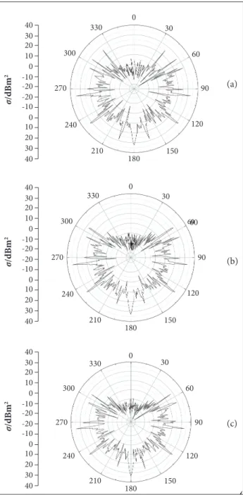
he leading edge’s sweep angle χ varies from 0° to 66°, at an interval of 3°, and consequently 23 kinds of 3-D digital prototypes of the variable-sweep wing aircrat can be obtained. When calculating each aircrat prototype’s RCS, the grids covering the whole aircrat are irstly generated, the radar incident wave is set to be at X band and of the horizontal polarization, and the pitching angle is 0°; 23 diferent characteristic curves of the aircrat’s RCS can then be obtained. In this series of numerical simulations, the variable-sweep wing aircrat’s grids are shown in Fig. 7, where χ is equal to39°, 54° and 66°, respectively, and the RCS characteristic curves for these three diferent variable-sweep wing aircrat are shown in Fig. 8.
σ
/dB
m
2
40 30 20 100 -10 -20 -20 -10 0 10 20 30
40 -5o
0o
5o
0
30
60
90
120
150 180
210 240 270
Figure 8. RCS characteristics in the type for χ of aircraft. (a) χ = 39°; (b) χ = 54°; χ = 66°.
Figure 7. Trellis diagram in the type for χ of aircraft.
(a) χ = 39°; (b) χ = 54°; (c) χ = 66°.
σ /dB m 2 40 30 20 100 -10 -20 -20 -10 0 10 20 30 40 σ /dB m 2 40 30 20 100 -10 -20 -20 -10 0 10 20 30 40 σ /dB m 2 40 30 20 100 -10 -20 -20 -10 0 10 20 30 40 0 30 60 90 120 150 180 210 240 270 300 330 0 30 60 90 120 150 180 210 240 270 300 330 0 30 60 90 120 150 180 210 240 270 300 330
From the data shown in Figs. 8a to 8c, we can obtain some conclusions here: (1) when the wing leading edge’s sweep angle is 39°, the RCS arithmetic average value between ± 10° of the aircrat is –1.02 dBm2, and the RCS arithmetic average value
between ± 30° of the aircrat is –1.61 dBm2. he RCS peak value,
appearing symmetrically in the aircrat’s head direction, is 24.85 dBm2 and appears at both +39° and –39° azimuth angles.
his proves that, in the head direction of the aircrat, the azimuth angle corresponding to the RCS peak value is equal to the wing leading edge’s sweep angle; (2) when the wing leading edge’s sweep angle is 54°, the RCS arithmetic average value between ± 10° of the aircrat is –5.901 dBm2, and the RCS arithmetic average
value between ± 30° of the aircrat is –5.59 dBm2. he RCS peak,
appearing symmetrically in the head direction of the aircrat, is 26.21 dBm2 and appears at both +54° and –54° azimuth angles.
his proves that, in the head direction of the aircrat, the azimuth angle corresponding to the RCS peak value is equal to the wing leading edge’s sweep angle; (3) when the wing leading edge’s sweep angle is 66°, the RCS arithmetic average value between ± 10° of the aircrat is –4.68 dBm2, and the RCS arithmetic average
value between ± 30° of the aircrat is –6.198 dBm2. he RCS
peak value appears twice symmetrically in the head direction of the aircrat, and the peak values are 27.72 and 25.1 dBm2, appearing
at both ± 55° and ± 66° azimuth angles. his proves that, in the head direction of the aircrat, the azimuth angle corresponding to the RCS peak value is equal to the wing leading edge’s sweep angle. For another RCS peak, the aircrat forward azimuth is equal to the horizontal tail leading edge sweep angle, which is ± 55°.
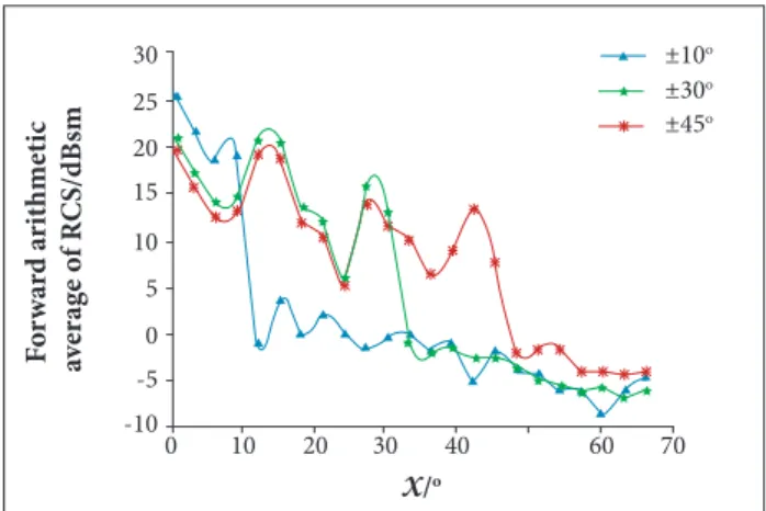
Based on the mathematical statistics and comparative analysis of all the 23 aircrat RCS characteristic curves obtained from the simulations, the relationship curve between the RCS peak value and the sweep angle χ is shown in Fig. 9, and the relationship curve between the corresponding azimuth angle of the aircrat RCS forward peak value and the sweep angle χ is shown in Fig. 10, the relationship curves between the aircrat RCS forward arithmetic average value and sweep angle χ are shown in Fig. 11. It can be seen from Fig. 9 that, when the wing leading edge’s sweep angle χ is 0°, its aircrat’s RCS forward peak value is 36.08 dBm2. When χ = 18°, its aircrat’s RCS peak value is
28.19 dBm2, and, ater unit conversion, we know that the
aircraft’s RCS peak value when χ = 18° is 16.25% of that when χ = 0°. When χ = 33°, its aircrat’s RCS peak value is 26.19 dBm2, and the converting results show that the aircrat
RCS peak value when χ = 33° is 10.25% of that when χ = 0°. When χ = 42°, its aircrat’s RCS peak value is 29.85 dBm2, and
Figure 9. Relation between aircraft’s RCS forward peak
value and χ.
Figure 11. Relation between aircraft’s RCS forward
arithmetic average value and χ.
Figure 10. Relation between the corresponding azimuth
angle of aircraft’s RCS forward peak value and χ.
X/o
F o rwa rd a ri thme ti c a ve rage o f R CS/dBs m 30 20 15 10 5 0 -5 -10
0 10 20 30 40
±10o ±30o ±45o 60 70 25 X / o
Azimuth of forward peak value for RCS/o 70 60 50 40 30 20 10 0
0 10 20 30 40 50 60 70
F o rwa rd p ea k va lu e o f R CS/dB m 2
X/o 38 34 30 26 22 18
0 10 20 30 40 50 60 70
the converting results show that, when χ = 42°, the aircrat’s RCS peak value is 23.82% of that when χ = 0°. When χ = 54°, its aircrat’s RCS peak value is 26.21 dBm2, and the converting
results show that the aircrat’s RCS peak value for χ = 54° is 10.30% of that when χ = 0°. When χ = 66°, its aircrat’s RCS peak value is 25.10 dBm2, and the converting results show
that the aircrat’s RCS peak value when χ = 66° is 7.97% of that when χ = 0°. It can be seen that, when the sweep angle of the aircrat increases, the peak value of the RCS decreases non-linearly.
Figure 10 shows that the azimuth angle corresponding to one of the RCS peak value is equal to the aircrat’s sweep angle.
From Fig. 11, we can see that:
• The arithmetic average value of the aircraft’s RCS between ± 10° is and, when χ = 0°, = 25.67 dBm2;
when χ = 33°, = 0 dBm2 and, ater unit conversion,
we know that when χ = 33°, is 0.271% of that when χ = 0°. When χ = 42°, = -4.97 dBm2, and when χ = 42°,
is 0.087% of that when χ = 0°.
• The arithmetic average value of the aircraft’s RCS between ± 30° is and, when χ = 0°, = 21.21 dBm2;
when χ = 33°, = -0.7 dBm2 and, ater unit conversion,
we know that, when χ = 33°, is 0.644% of that when χ = 0°; when χ = 42°, = -2.67 dBm2 and, when χ = 42°,
is 0.409% of that when χ = 0°.
• The arithmetic average value of the aircraft’s RCS between ± 45° is and, when χ = 0°, = 19.53 dBm2;
when χ = 33°, = 10.07 dBm2 and, when χ = 33°,
is 11.324% of that when χ = 0°. When χ = 42°, = 13.39 dBm2 and, when χ
= 42°, is 24.32% of that when χ = 0°.
CALCULATING THE RADAR DETECTION PROBABILITY
he purpose of studying the RCS characteristics of the variable-sweep wing aircrat is to reduce the detection probability by the hostile radar. In this section, we study the relationship between the detection probability and the characteristics of the target’s RCS and the detection distance.
In a typical ground-to-air searching situation, as mentioned in section Radar Detection Probability Model, the rolling and azimuth angles of the incident wave relative to the aircrat are both 0°, and βf, hd, hm of Eqs. 8 and 9 are set to be –2.5°, 8 km, and 3 km, respectively. Figure 12 shows the relationship between the pitching angle of the incident wave and the detection distance. As shown in Fig. 12, β decreases from –5° to below –30° when the detection distance decreases from 200 to 0 km. The corresponding RCS values of the aircraft under these attitudes can then be calculated using the PO method and
±10o σt ±10o σt ±10o σt ±10o σt ±10o σt ±10o σt ±30o σt ±30o σt ±30o σt ±30o σt ±30o σt ±30o σt ±45o
σt ±45o
Figure 14. Detection probability of the aircraft when it is lying from 200 km away.
Figure 12. The pitching angle of the incident wave against
the detection distance.
0.0
0 50 100 160 200
0.2 0.4 0.6 0.8 1.0
R/km
PDk
X = 15o
X = 39o
X = 54o
0 -35 -30 -25 -20 -15 -10 -5 0
50 100 150 200
R/km
β
/
o
40 -40 -30 -20 -10 0 10 20
80 120 160 200
R/km
σ
/dB
m
2
X = 15o
X = 39o
X = 54o
Figure 13. The RCS of variable-sweep wing aircraft against
detection distance.
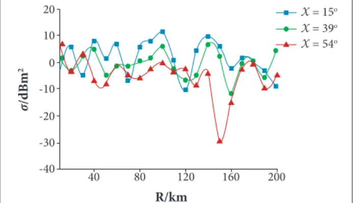
ECM. he incident wave is at X band and of horizontal polarization. Figure 13 shows the varying RCS value of the aircrat when it is lying towards the searching radar from 200 km away. hree types of lines indicate three diferent sweep angles, which are χ = 15°, 39° and 54°, respectively.
Figure 13 shows that, when the aircrat is lying towards the radar from 200 km away, its RCS value varies between about –20 and 10 dBm2.
According to the RCS values shown in Fig. 13, the detection probability can be calculated using Eq. 7. The initial parameters of the pulse Doppler radar are set as follows: Δθα = 7°, fr = 300 Hz, Ω = 30°/s, Pt = 10 MW, G = 36 dB, λ = 0.03 m, E = 900, Bn = 0.077 MHz, Fn = 55 dB, L = 20 dB. RCS values of Fig. 13 are expressed in dBm2, when
applied to Eq. 7, they should be converted to m2, with
the help of Eq. 6. Figure 14 shows the calculation results of the aircraft’s detection probability.
As shown in Fig. 14, when the aircrat is lying right towards the radar from 200 km away, the detection probabilities are very low when R is beyond about 120 km, for all 3
types of variable-sweep wing aircrats. When the distance decreases to within 100 km, the aircrat with a sweep angle of χ = 54° performs best and the aircrat with a sweep angle of χ = 15° performs worst. When the distance decreases to within 40 km, all 3 types of variable-sweep wing aircrats perform almost the same.
CONCLUSION
his paper utilizes the physical optics and the equivalent currents methods to study the RCS characteristics of the variable-sweep wing aircrat. Based on the numerical simulations of the aircrat, the following conclusions can be obtained:
he aircrat’s RCS forward peak value decreases non-linearly with the sweep angle χ.
he sweep angle of the variable-sweep wing aircrat and the azimuth angle corresponding to one of the RCS peak values are identical.
When χ = 33°, = –0.7 dBm2. Ater unit conversion,
of the aircrat when χ = 33° is 0.644% of that when χ = 0°. he larger the sweep angle of the variable-sweep wing aircrat is, the lower the aircrat’s detection probability will be. We hope that the conclusions of this paper provide some reference and technical support for stealth aircrat’s demonstration and designing.
ACKNOWLEDGEMENT
his work was supported by the Natural Science Foundation of China (51375490).
±30o
σt
±30o
REFERENCES
Bai, Z.D. and Liu, H., 2007, “Parametric Modeling and Optimization of Observability Fuselage in Aircraft Conceptual Design”, Journal of Beijing University of Aeronautics and Astronautics, Vol. 33, No. 12, pp. 1391-1394.
Bao, J.B. and Wang, G.L., 2012, “Optimization and Experimental Veriication for Aerodynamic Scheme of Flying-Wing”, Journal of Beijing University of Aeronautics and Astronautics, Vol. 38, No. 2, pp. 180-184.
He, X., Chen, J.P. and Ni, X.W., 2010, “Attenuation of Planar Electromagnetic Waves by Inhomogeneous Plasma”, High Power Laser and Particle Beams, Vol. 22, No. 9, pp. 2115-2118.
Hu, T.Y. and Yu, X.Q., 2011, “Preliminary Design of Unconventional Coniguration Aircraft Using Multidisciplinary Design Optimization”, Acta Aeronautica et Astronautica Sinica, Vol. 32, No. 1, pp. 117-127.
Huang, P.L. and Liu, Z.H., 2008, “Research on Electromagnetic Scattering Characteristics of Slits on Aircraft”, Acta Aeronautica et Astronautica Sinica, Vol. 29, No. 3, pp. 675-680.
Ji, J.Z., Wu, Z. and Liu, Z.H., 2009, “Research on the Curvature Parameter in the S-Shaped Inlet’s Stealth Design”, Journal of Xidian University, Vol. 36, No. 4, pp. 746-750.
Lu, J.W. and Wang, Qi., 2009, “Aircraft-Skin Infrared Radiation Characteristics Modeling and Analysis”, Chinese Journal of Aeronautics, Vol. 22, No. 5, pp. 493-497.
Nangia, R.K. and Palmer, M.E., 2005, “A Comparative Study of UCAV Type Wing Planforms--Aero Performance and Stability Considerations”, AIAA-2005-5078.
Sun, C. and Zhang, P., 2008, “LO Requirements and Solutions of Avionics/RF System for Advanced Aircraft”, Acta Aeronautica et Astronautica Sinica, Vol. 29, No. 6, pp. 1472-1481.
Tom, R.B. and Alfred, G.S., 2010, “Optimization of Aircraft Coniguration for Minimum Drag”, AIAA-2010-3000.
Vogel, B.S., 2005, “Boeing X-45 UCAVs Complete Simulated Mission”, Janes Defence Industry, UK.
Wood, R.M. and Bauer, S.X.S., 2001, “Flying Wings/Flying Fuselage”, AIAA-2001-0311.
Yue, K.Z., Hou, Z.Q. and Yang, Y.K., 2010, “Markov Model of Eficiency of Volleying Anti-Ship Missiles Piercing into Ship-Bone Antiaircraft Missiles”, Journal of System Simulation, Vol. 22, No. 6, pp. 1472-1475.
Yue, K.Z., Liu W.L., Li G.X., Ji J.Z. and Yu D.Z., 2015, “Numerical Simulation of RCS for Carrier Electronic Warfare Airplanes”, Chinese Journal of Aeronautics, Vol. 28, No. 2, pp. 545-555.
Yue, K.Z., Gao, Y., Li, G.X. and Yu, D.Z., 2014a, “Conceptual Design and RCS Performance Research of Shipborne Early Warning Aircraft”, Journal of Systems Engineering and Electronics, Vol. 25, No. 6, pp. 968-976.
Yue, K.Z., Sun, C. and Ji, J.Z., 2014b, “Numerical Simulation on the Stealth Characteristics of Twin-Vertical-Tails for Fighter”, Journal of Beijing University of Aeronautics and Astronautics, Vol. 40, No. 2, pp. 160-165.
Yue, K.Z., Sun, C., Liu, H. and Su, M., 2014c, “Numerical Simulation on the RCS of Combat Aircraft for Mounted Missile”, Systems Engineering and Electronics, Vol. 36, No. 1, pp. 62-67.