Ediguer E. Franco
[email protected] Universidad Autónoma de Occidente Departamento de Energética y Mecánica Cll 25 #115-85 Cali, Valle del Cauca, ColombiaMarco A. B. Andrade
[email protected]Julio C. Adamowski
[email protected]Flávio Buiochi
[email protected] Escola Politécnica da Universidade de São Paulo Departamento de Engenharia Mecatrônica e de Sistemas Mecânicos 05508-030 São Paulo, SP, BrazilAcoustic Beam Modeling of
Ultrasonic Transducers and Arrays
Using the Impulse Response and the
Discrete Representation Methods
The impulse response of the velocity potential and the discrete representation methods were used in order to model the acoustic field radiated by ultrasonic transducers and arrays. The first method deals with the calculation of the exact impulse response, in which solutions are possible only for simple geometries, such as the circular piston. The second method is an approximated solution based on the discretization of the acoustic aperture in small elementary areas, each of them radiating a spherical wave. By using circular transducers, which can be considered circular pistons, many simulations comparing the methods were carried out. The relation between the computational cost and the precision was analyzed, thus establishing the time and space discretization levels. The simulations were made using the Matlab software and the results were compared to experimental measurements showing good agreement. The experimental results were obtained using a scanning system. The acoustic field radiated from a 1 MHz circular transducer was measured as well as a 3.5 MHz array of 16 elements both immersed in water. The acoustic field radiated by the array was simulated and measured with focalization on a radius of 30 mm with deflections of 0° and 20°.
Keywords: acoustic field, ultrasonic transducer, array, impulse response, discrete representation method
Introduction1
Acoustic beam modeling of ultrasonic transducers consists of the determination of the acoustic pressure at a point or a region in front of the radiating surface. By the study and implementation of mathematical models, wave propagation is analyzed in nondestructive testing in order to optimize design parameters, such as geometry, focus depth, acoustic beam width and directivity. The acoustic beam generated is mainly dependent on the transducer geometry, the properties of the propagating medium and the excitation pulse form.
The acoustic beam generated by an ultrasonic transducer can be modeled using the Rayleigh and Rayleigh-Sommerfeld equations (Goodman, 2004), which describe the acoustic propagation phenomenon in an integral form. From the Rayleigh-Sommerfeld equations, two methods for calculating the acoustic beam were developed. The first method is an exact solution for apertures with a simple geometrical shape and the second one is a numerical approximation that allows the analysis of arbitrarily shaped apertures.
The most used method to calculate the exact solution is based on the temporal impulse response of the velocity potential. This method permits to calculate, in the time domain, the acoustic pressure induced in the medium by the transducer in an arbitrary spatial point. The method was initially proposed in acoustics by Stephanishen (Stephanishen, 1971) and, in order to obtain the exact solution of the impulse response, it is necessary to calculate complex integrals, only possible in the simplest geometry cases: circular pistons (Lockwood and Willette, 1973; Djelouah and Baboux, 1992), rectangular transducers (San Emeterio and Gómez-Ullate, 1992), triangular apertures (Jensen, 1996) and ring segments (Martínez et al., 2001).
In the complex geometry cases, a relevant method is the discrete representation proposed by Piwakowski and Delannoy (1989), which consists in dividing the irradiating surface into small area elements, each of them irradiating a semi-spherical wave (Huygens principle). The superposition of all semi-spherical waves approaches the exact solution when the area elements become smaller. The
Paper received 20 May 2009. Paper accepted 10 August 2011. Technical Editor: Domingos Rade
discrete method permits to analyze different transducer geometries (Jensen and Svendsen, 1992) and inherent problems of the acoustic beam generation (Piwakowski and Sbai, 1999). Moreover, the method can be used to investigate acoustic beams when transmission and reflection phenomena are involved (Buiochi et al., 2004; Belgroune et al., 2008).
The acoustic beam generated depends on the emitted wave type (Weight, 1984). Excitation can be in continuous mode by using an electrical sine signal or in transient mode by means of an electrical pulse of short duration. Both excitation modes can be applied in the simulations of the acoustic beam by using the impulse response and discrete representation methods. However, in this work, only the transient excitation was used due to its important applications in nondestructive testing by ultrasound.
Ultrasonic transducers can be either mono-element or multi-element. The mono-element transducers have only one active element generally made of a piezoelectric material. The mono-element transducer is widely used in nondestructive testing and characterization of solids and liquids. That transducer has a fixed focus that has to be translated to generate an image. The plane piston transducer has a natural focus in a spatial point that is a function of its operation frequency and its radius. That natural focus can be modified by acoustic lens. The multi-element transducer is an array of active elements working independently. The main advantage of the ultrasonic arrays consists in the generation of an image avoiding the transducer translation. This is possible due to the capability of deflecting the acoustic beam and the dynamic modification of the focus. It is thus possible to avoid the complex mechatronic system required for controlling the transducer position.
Nomenclature
a = plane piston radius, m
aj = impulse response of the velocity potential generated by each elementary surface
A = apodization function, dimensionless c = propagation velocity, m/s
e = root mean square error factor f = frequency, Hz
h = impulse response of the velocity potential
h = temporal mean of the discrete impulse response p = pressure, Pa
r = distance between the point P and a specific point on the aperture surface, m
R = distance from the center of the array to the focus, m S = total acoustic aperture area, m2
t = time, s
T = delay function, s v = particle velocity, m/s
xn = distance from the center of the array to the element, m Greek Symbols
α = boundary conditions coefficient
δ = Dirac’s delta function
φ = deflection angle, degree
Φ = velocity potentia, l
λ = wave length, m
ρ = density, kg/m3
θ = angle between the vector and the normal vector to the emitter surface, degree
Ω = angles of the arcs on the piston surface, degree Subscripts
a,P = spatial points
d = discrete representation
Theoretical Background
Rayleigh and Rayleigh-Sommerfeld equations
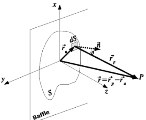
Figure 1. Geometry and notation used in the Rayleigh and Rayleigh-Sommerfeld equations.
By considering the acoustic wave propagation in an adiabatic medium and supposing small particle displacements, the linear equation of the instantaneous pressure (p) in an isotropic, non-viscous, homogeneous and perfectly elastic medium is (Stephanishen, 1971):
( )
( )
t t , r Φ ρ = t , r p P P ∂ ∂ r r (1)where rp r
is the position vector of the point P where the pressure is
calculated, as shown in Fig. 1, ρ is the medium density and Φ
( )
rP,tr
is the velocity potential defined as:
( )
r ,t = Φ( )
r ,t vr rP rP−∇ (2)
where v
( )
rP,t r ris the particle velocity.
When the acoustic aperture is surrounded by a rigid baffle, the space-time dependence of the acoustic beam can be modeled by the Rayleigh integral (Stephanishen, 1971). That integral represents the velocity potential in a point of the acoustic beam as the sum of the infinite contributions of individual acoustic sources of area dS, each of them irradiating a semi-spherical wave into the medium (Huygens’ principle):
( )
∫
(
−)
S a n P dS r c r t , r v π = t , r Φ / 2 1 r r (3)where r is the distance between point P in the acoustic beam and the elementary area dS (
r
ar
), c is the wave propagation velocity in the
medium, S is the active area of the transducer and vn
( )
ra,t ris the normal component of the velocity at each point on the transducer surface. The particle velocity is zero at all points on the rigid baffle; in this case, by using Eq. (1), the acoustic pressure at the point P is:
( )
∂∂∫
(
−)
S a n P dS r c r t , r v t π ρ = t , r p / 2 r r (4)When the acoustic aperture is surrounded by a soft baffle, pressure is zero at all surrounding points, the pressure at each point into the acoustic beam can be represented by the Rayleigh-Sommerfeld integral:
( )
p(
r ,t r c)
dSt r θ πc = t , r p S a
P
∫
−∂ ∂ / cos 2 1 r r (5)
where θ is the angle of vector rr
with respect to the normal vector (n
r
) of the irradiating area element, and p
( )
ra,tr
is the pressure at each point on the acoustic aperture. It can be seen that the acoustic beam is a result of the superposition of waves.
Impulse response method
The impulse response method separates the effect induced by the geometry from the effect induced by the time-dependent excitation. This permits to obtain the exact solution of the Rayleigh integral (Stephanishen, 1971). By considering an acoustic aperture (Fig. 1) surrounded by a rigid baffle, irradiating into an isotropic lossless medium and supposing in-phase motion at all points on the acoustic aperture, the normal velocity in the point ra
r
can be represented by:
( ) ( ) ( )
r,t =Ar vt vnr
ar
awhere A
( )
ra ris the apodization factor that determines the distribution of the vibration amplitudes on the emitter surface and
( )
tv is the time-dependent excitation. Then, the Rayleigh integral can be reduced by expressing the velocity potential as a convolution of two functions:
( ) ( ) ( )
r ,t =vt h r ,tΦ P P
r r
∗ (7)
where h
( )
rP,tr
is the impulse response of the velocity potential given by:
( )
∫
( ) (
−)
S a a P dS r c r t , r δ r A π = t , r h / 2 1 r r r (8)where δ
( )
is the Dirac’s delta function. The acoustic pressure at point P can be obtained by associating (1), (7) and (8).Exact solution in the plane circular piston case
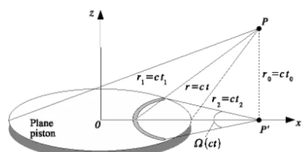
Figure 2. Geometry and notation used in the exact solution of the circular piston.
For a uniformly excited circular piston radiating into a lossless medium, the Rayleigh integral can be reduced from a surface integral to a simple integral by using cylindrical coordinates and variable substitution (Robinson et al., 1974). Then, the analytic exact solution of the velocity potential impulse response at point P in front of the acoustic aperture is obtained, according to:
( )
( )
otherwise 0 if 2 2 1<t<tt ct Ω π c = t , r h rP
(9)
where c is the propagation velocity of the wave and Ω
( )
ct is the angle of the arcs centered at point P’ (the projection of point P on plane z = 0) limited by the piston edge, as shown in Fig. 2. The concentric arcs are formed by the impulsive excitation of points on the piston surface that reach point P at the time t=r/
c, where r is the distance between point P and the points of the arc. It can be noted that r1 and r2 denote, respectively, the larger and smaller distances between point P and the piston surface. Then, t1=r1/cand t2=r2/c are the times that limit the transient field and the
duration of the impulse response is t2−t1.
In the case of a circular piston of radius a, the expressions for the angles of the arcs on the piston surface (Ω
( )
ct ) are shown inTable 1 (Robinson et al., 1974). The piston is divided into three regions: inside, on the edge and outside the piston surface, where x, y and z are the Cartesian coordinates of point P and the times t0, t1 and t2 are defined as:
c z
t0
=
/c z x a t 2 2 1 ) ( − + = (10) c z x a t 2 2 2 ) ( + + =
Table 1. Expressions for the angles of the arcs on the piston surface.
Region on the piston surface
( )
ctΩ Time interval
Inside 0 t<t0 or t>t2
(x < a) 2 π
1 0 t t
t ≤ ≤
− − − − 2 2 2 2 2 2 2 2 1 2 2cos z t c x a x + z t
c t1<t≤t2
On the edge
0
2 0 or t>t
t < t
(x = a) π
1 0 or t=t
t = t − − a z t c 2 2cos 2 2 2
1 t1<t≤t2
Outside 0
2 1 or t>t
t t≤
(x > a)
− − − − 2 2 2 2 2 2 2 2 1 2 2cos z t c x a x + z t
c t1<t≤t2
Discrete representation method
The discrete representation is an approximated method suitable for both mono-element apertures (Piwakowski and Delannoy, 1989) and arrays (Piwakowski and Sbai, 1999). The accuracy of the results depends strongly on the temporal and spatial resolutions used in the model. By considering the three contour cases: rigid baffle, soft baffle and free field, the impulse response function presented by Piwakowski and Delannoy (1989) and based on the work of Lasota et al. (1984) is:
( )
∫
( ) ( )
[
−
−
( )
]
S a a PdS
r
r
T
c
r
t
δ
θ
α
r
A
π
=
t
,
r
h
r
r
r
/
2
1
(11)where
A
( )
r
a ris the apodization function that represents the amplitude of the semi-spherical wave generated by each elementary area dS, T
( )
rar
is the excitation delay function defined at each point
on the emitter surface, θ is the angle between the vector
r
ra and the( )
( )
( )
[
]
field Free 2 / cos 1
bafle Soft cos
baffle Rigid 1
θ
+
θ
=
θ α
(12)
Equation (11) is more general than Eq. (8), where the factor that takes into account the different cases of boundary was included, as well as the delay function used in the focalization of arrays.
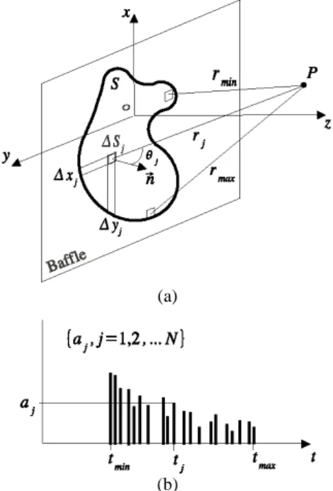
As shown in Fig. 3a, the emitter surface can be discretized in N elementary areas ∆Sj=∆xj∆yj, j = 1,2...N, where
j j
S
∆
=
S
∑
.Then, the integral in Eq. (11) can be replaced with the sum of the contributions of each elementary area. Those contributions are computed as the velocity potential generated by each elementary area that reaches point P at instant t, according to:
( )
[
]
jj j j j N
j j P
d ∆S
r T c r t
δ α
A
π
= t , r
h
∑
− / −2 1 r
(13)
where
h
d( )
r
P,
t
r
is the discrete representation of the impulse
response at each instant t = rj/c+Tj,
r
j is the distance between point P and each elementary area∆S
j,A
j andT
j are the discretevalues of the functions A
( )
ra rand T
( )
ra r, respectively, and αj is the boundary conditions coefficient.
(a)
(b)
Figure 3. a) Notation used in Eq. (13) and b) graphic representation for aj.
The discrete impulse response becomes a sequence of Dirac pulses, as shown in Fig. 3b. It can be seen that tmin and tmax are,
respectively, the smallest and largest propagation times between the elementary area and point P. The amplitude factor aj represents the impulse response of the velocity potential generated by each elementary surface ∆Sj:
j j j j j
πr
∆S α
A = a
2 (14)
Then, if time is discretized using intervals with duration ∆t and the temporal mean of all amplitudes a that reach the point P into a j
temporal window
[
ts−∆t/2,ts+∆t/2]
is calculated, the mean impulse response at the time ts is:( )
1
for
/
2
/
2
1
∆
t
+
t
<
t
<
∆
t
t
a
∆
t
=
t
,
r
h
s j sN
= j
j s
P
d
∑
−
r
(15)
In Fig. 4, series aj, the temporal mean of the discrete impulse response hd and the exact impulse response h at the time ts are graphically shown. hd approaches the exact analytic solution h for the frequency spectrum f<fmax, where fmax<<1/∆t, when the size of the elementary areas becomes smaller (Piwakowski and Sbai, 1999), in such a way that:
(
)
d(
P s)
∆S s
P,t = h r ,t
r
h r r
lim 0
→ (16)
Figure 4. Graphic representation of hd.
The temporal mean of the impulse response
h
d is the computational approximated solution used in this work, the temporal and spatial samplings are ∆t and∆
x
j=
∆
y
j, respectively. Then, by using Eqs. (1) and (7), the pressure at the point P can be calculated by:( )
( ) ( )
h r ,tt t v
ρ
= t , r
p rP d rP
∗ ∂ ∂
(17)
Linear array focalization
intensities are smaller and even null at certain points due to destructive interference (Parrilla, 2004).
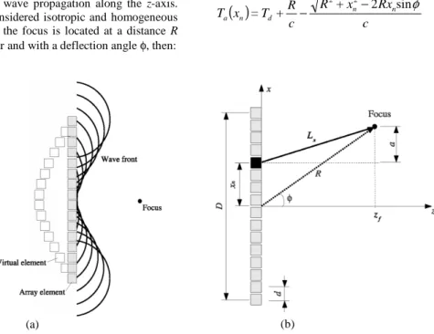
In practice, focalization is obtained by adjusting the propagation times between each element and the focus. This principle is shown in Fig. 5a, where the virtual elements represent the delays in the propagation time. Then, the wavefront advances as generated by a transducer with acoustic lens and all the semi-spherical waves reach the focus simultaneously.
The geometry and the axis coordinate system used to obtain the delay times are represented in Fig. 5b. The transducer is placed throughout the x-axis, and the wave propagation along the z-axis. The propagation medium is considered isotropic and homogeneous with propagation velocity c. If the focus is located at a distance R from the center of the transducer and with a deflection angle φ, then:
φ
sin 2 2 2n n
x= R +x Rx
L − (18)
The excitation of each element is delayed so that all waves reach the focus at the same time t=R/c+Td, where T is a positive d arbitrary constant introduced to avoid negative delay times. Thus, the function that supplies the delays can be obtained from Eq. (18):
( )
c Rx x + R c R + T = x
T n n
d n a
φ
sin 2 22 −
−
(19)
(a) (b)
Figure 5. Array focalization: (a) principle and (b) geometry used in order to obtain Eq. (19).
Experimental and Theoretical Results
Plane piston
Simulations of the waveform and the acoustic beam generated by a 19-mm diameter circular plane piston were carried out by using the Matlab software. Results obtained using the exact solution and the discrete representation method were compared by considering 6 different cases. The propagating medium is water (ρ = 1000 kg/m, c = 1480 m/s) and the excitation signal corresponds to a 1 MHz (λ = 1.5 mm) sine burst of 5 cycles. Rigid baffle was the boundary condition used in the models.
In order to analyze the relative error between the exact and discrete solutions, a root mean square factor of the signals (pressure response) was calculated, as follows:
( )
( )
[
]
∑
N −= i
D
E i S i
S N = e
1
2 1
(20)
where SE
( )
i and SD( )
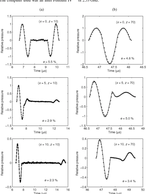
i are the signals calculated by the exact solution and the discrete representation method, respectively, and N is the number of temporal points used (sampling). As both signals are normalized to their maximum value, the error can be represented in percentage.Figure 6 compares the pressure response obtained using the exact solution (continuous line) and the discrete representation
method (dashed line) at six points in plane y = 0. The origin of the coordinate system is in the piston center and the positive z-axis is the direction of the acoustic propagation, as depicted in Fig. 3. The pressure responses were obtained in the two different regions of the acoustic beam: near field and far field. Near field is the region straight ahead of the ultrasonic transducer and it is characterized by many constructive and destructive interferences. These interferences lead to many fluctuations in the acoustic pressure near the ultrasound transducer. Far field occurs in the region beyond the near field, and it is characterized by small fluctuations of the sound pressure. Figure 6a shows the results corresponding to three points in the near field (z = 10 mm): on the acoustic axis (x = 0 mm) and off the acoustic axis (x = 5 and x = 10 mm). Figure 6b shows the results in the far field (z = 70 mm) for the same positions. Moreover, the relative error between both solutions, calculated by Eq. (20), is plotted in the figure. In the discrete representation method a space discretization of ∆x=∆y=λ/8 and a time discretization of
30 / λ
= ∆t
c were used.
transducer was found. The computer used was an Intel Pentium IV of 2.53 GHz.
(a) (b)
Figure 6. Pressure response comparison for the exact solution (solid line) and the discrete representation method (dashed line) in the regions: (a) near field (z = 10 mm) and (b) far field (z = 70 mm).
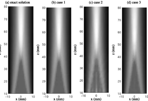
Table 2. Spatial and temporal discretization used and the CPU time required to calculate the fields shown in Fig. 7.
Case ∆x=∆y (mm) c∆t (mm) CPU Time (s)
Exact - λ/120 2
1 λ/16 λ/120 1240
2 λ/2 λ/120 21
Figure 7. Comparison between the pressure fields obtained using the exact solution and the discrete representation for the three different cases shown in Table 2. (The clearest areas represent the maximum peak-to-peak pressure).
Figure 8. Acoustic field (a) experimental, (b) calculated by the discrete representation method and (c) calculated by the exact solution. (The clearest areas represent the maximum peak-to-peak pressure).
The acoustic beam irradiated in water by a circular 19-mm 1 MHz ultrasonic transducer was experimentally measured. A 0.4-mm diameter hydrophone was used as the receiver. A computerized system automatically scanned the field and saved the data in a suitable format for further processing. The pressure amplitude, measured and simulated, at each point in the field was taken as the peak-to-peak value of the obtained wave.
Figure 8 compares the experimental field measured to the theoretical ones obtained with the exact and discrete solutions. The amplitude values of each field were normalized to its maximum value. The exact solution was calculated with a temporal discretization of c∆t=
λ
/30 and the approximated solution with the same temporal discretization and a spatial discretization of8 / λ
=
∆y
=
∆x . Figure 9 shows the pressure amplitude profiles of the acoustic experimental, exact and approximated fields calculated in the near field (z = 10 mm) and in the far field (z = 70 mm).
As it can be seen, the computational methods show a good fit when compared to the experimental field. Some differences can be explained by the excitation wave, which was measured by the hydrophone at 5 mm from the transducer surface, where only the component of the plane wave was used. Nevertheless, those models are appropriate to determine the acoustic field generated by a plane piston transducer.
Transducer arrays
become greater when the deflection angle grows. Thus, for a frequency f0 = 3.5 MHz and propagation velocity of 1480 m/s in water, the wavelength is λ = 0.423 mm and the array element width is of the same order (d≈λ/2).
Figure 9. Comparison of the experimental, exact solution and discrete representation pressure amplitudes in (a) z = 10 mm and (b) z = 70 mm for
| |
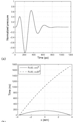
x≤10 mm.Figure 10(a) shows the waveform used in the simulation as the excitation input. It is an asymmetric ultrasonic pulse of 3.5 MHz with normalized amplitude.
The surface of each element was discretized by square elementary areas of ∆S = 0.01 mm. The temporal discretization was 1/18 times the period of the excitation waveform; therefore, the sampling frequency was fs=18f0=63 MHz, which is sufficient to embrace
all the excitation waveform spectra. The choice of ∆S and fs is an important task because coarse discretizations can lead to poor results and fine discretizations lead to excessive processing time. In addition, the selection of the number of points of the calculated field is also important. In order to obtain a good resolution in the acoustic field, 8000 points were used, 80 points being in the x direction and 100 in the propagation direction (z). Experimental fields were measured with smaller resolution: 30 points in the x direction and 133 in the z direction, totalizing 3990 points.
(a)
(b)
Figure 10. (a) Waveform and (b) time delays used in the simulations.
Figure 10(b) shows the delay times used in the simulation. The values were calculated from Eq. (19). Two cases were considered: focalization in R = 30 mm without deflection (φ = 0°) and focalization in R = 30 mm with deflection of 20 degrees (φ = 20°). The maximum delay time in the case with deflection is ten times higher than the other case.
The experimental field was measured at the Instituto de Automática Industrial–CSIC, in Spain. A 0.2-mm diameter hydrophone, an automated system for the hydrophone positioning and an acquisition data system were used.
Figure 11. Irradiated pressure field with focalization in R = 30 mm without deflection: (a) experimental and (b) simulated. (The clearest areas represent the maximum peak-to-peak pressure).
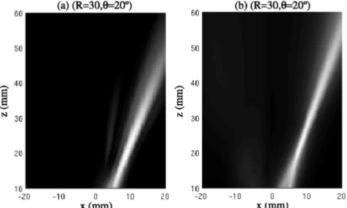
distribution in the real transducers surface, that is, all the points in the surface do not vibrate in phase or with the same amplitude. On the other hand, time delays must be calculated with high precision and frequently that is not possible due to hardware limitations. The difference in the discretization used in the simulated and experimental cases also cause problems in the obtained fields. Figure 12 presents the results obtained for focalization at the point (R = 30 mm, φ = 20°), showing good agreement.
Figure 12. Irradiated pressure field with focalization on R = 30 mm and deflection of 20°: (a) experimental and (b) simulat ed. (The clearest areas represent the maximum peak-to-peak pressure).
Conclusions
Rayleigh and Rayleigh-Sommerfeld integral equations are effective for modeling the acoustic beam radiated by ultrasonic transducers. Exact solutions for some simple geometry are possible and a discrete method, based on the same equations, allows the computations for complex geometries.
The exact solution for the plane piston was used in order to analyze the computational cost involved in the discrete solution. The time required by different discretization cases was compared to that obtained with the exact solution. As expected, high temporal and spatial discretizations increase the CPU time. A test is necessary to select the appropriate discretization; nevertheless, the discretization used in order to generate the pressure responses shown in Fig. 6 should be sufficient for most cases with a moderate increase in the CPU time.
The acoustic beam generated by a circular plane piston was measured and compared to the results obtained by the exact and discrete solutions. Both exact and discrete solutions provide a good reproduction of the experimental beam measured, although some slight differences can occur due to non-ideal effects, as discussed below.
Array focalization is a simple concept that can be easily simulated by the discrete representation method. This method is important because it allows analyzing the incidence of the deflection angle and the focus depth on the acoustic beam generated. Moreover, the effect of geometrical parameters, bandwidth, excitation and some non-ideal effects can be analyzed. The simulations reproduced the beams measured with good accuracy.
In both cases, plane piston and arrays, the differences between the simulated and measured cases are explained by non-ideal
effects. The most important is the presence of other vibration modes (such as surface and radial modes) in the real transducers, causing an out-of-phase motion of the points on the transducer surface. Other non-ideal effects are the fact that the surrounding baffle is not perfectly rigid, as assumed in the model, and the presence of matching layers on the irradiating surface. All these effects distort the acoustic beam.
Acknowledgments
The authors thank the Brazilian government institutions Capes, Fapesp and CNPq for the financial support that made this work possible, and the “Instituto de Automática Industrial – CSIC”, Spain, for the measurement of the acoustic beams with arrays.
References
Belgroune, D., Belleval, J.F., and Djelouah, H., 2008, “A theoretical study of ultrasonic wave transmission through a fluid-solid interface”,
Ultrasonics, 48, Issue 3, pp. 220-230.
Buiochi, F., Martínez, O., Gómez-Ullate , L., and Montero de Espinoza, F., 2004, “A computational method to calculate the longitudinal wave evolution caused by interfaces between isotropic media”, IEEE Trans.
Ultrason., Ferroelect., Freq. Contr., Vol. 51, No. 2, pp. 181-192.
Djelouah, H. and Baboux, J.C., 1992, “Transient ultrasonic field radiated by a circular transducer in a solid medium”, J. Acoust. Soc. Amer, Vol. 92, Issue 5, pp. 2932-2941.
Goodman, J.W., 2004, “Introduction to Fourier Optics”, third edition, Ed. Roberts & Company, 491 p.
Jensen, J.A., 1996, “Ultrasound field from triangular apertures”, J. Acoust.
Soc. Amer., Vol. 100, Issue 4, pp. 2049-2056.
Jensen, J.A. and Svendsen, N.B., 1992, “Calculation of pressure fields from arbitrarily shaped, apodized and excited ultrasound transducers”, IEEE
Trans. Ultrason., Ferroelect., Freq. Contr., Vol. 39, No. 2, pp. 262-267.
Lasota, H., Salamon, R., and Delannoy, B., 1984, “Acoustic diffraction analysis by the impulse method: A line impulse response approach”, J.
Acoust. Soc. Amer., Vol. 76, Issue 1, pp. 280-290.
Lockwood, J.C. and Willette, J.G., 1973, “High-speed method for computing the exact solution for the pressure variations in the nearfield of a baffled piston”, J. Acoust. Soc. Amer., Vol. 53, Issue 3, pp. 735-741.
Martínez, O., Gómez-Ullate, L. and Montero de Espinosa, F.R., 2001, “Computation of the ultrasonic field radiated by segmented-annular arrays”,
Journal of Computational Acoustics, Vol. 9, No. 3, pp. 757-772.
Parrilla, M.R., 2004, “Conformación de haces ultrasónicos mediante muestreo selectivo con codificación delta”, PhD thesis, Universidad Politécnica de Madrid, Madrid, Spain, 245 p.
Piwakowski, B. and Delannoy, B., 1989, “Method for computing special pulse response: Time domain approach”, J. Acoust. Soc. Amer., Vol. 86, Issue 6, pp. 2422-2432.
Piwakowski, B. and Sbai, K., 1999, “A new approach to calculate the field radiated from arbitrarily structured transducer arrays”, IEEE Trans.
Ultrason., Ferroelect., Freq. Contr., Vol. 46, No. 2, pp. 422-439.
Robinson, D.E., Less, S. and Bess, L., 1974, “Near field transient radiation patterns for circular pistons”, IEEE Transansactions on Acoustics,
Speech and Signal Processing, Vol. 22, No. 6, pp. 39-403.
San Emeterio, J.L. and Gómez-Ullate, L., 1992, “Diffraction impulse response of rectangular transducers”, J. Acoust. Soc. Amer., Vol. 92, Issue 2, pp. 651-662.
Stephanishen, P.R., 1971, “Transient radiation from pistons in an infinite planar baffle”, J. Acoust. Soc. Amer., Vol. 49, Issue 5B, pp. 1629-1638.
Weight, J.P., 1984, “Ultrasonic beam structures in fluid media”, J. Acoust.