Detection of determinant genes and diagnostic via Item Response Theory
Héliton Ribeiro Tavares
1, Dalton Francisco de Andrade
2and Carlos Alberto de Bragança Pereira
3 1Universidade Federal do Pará, Departamento de Estatística, Belém, PA, Brazil.
2
Universidade Federal de Santa Catarina, Departamento de Informática e Estatística,
Florianópolis, SC, Brazil.
3
Universidade de São Paulo, Departamento de Estatística, São Paulo, SP, Brazil.
Abstract
This work presents a method to analyze characteristics of a set of genes that can have an influence in a certain anomaly, such as a particular type of cancer. A measure is proposed with the objective of diagnosing individuals regarding the anomaly under study and some characteristics of the genes are analyzed. Maximum likelihood equations for general and particular cases are presented.
Key words:Item Response Theory (IRT), predisposition, propensity, logistic model.
Received: September 22, 2003; Accepted: May 12, 2004.
Introduction
In many practical situations, decisions have to be taken based upon individual quantities that cannot be ob-served directly. These quantities are referred to by latent variables that are given different names according to the ar-eas in which they are applied:abilityorproficiencyin edu-cational and psychological areas; purchasing power in marketing;life qualityorpredispositionto a certain disease in the biological and medical areas (see Andradeet al., (2000), Paas (1998), for example). These types of analysis are, in general, based upon the responses of a set of vari-ables often referred to asitemsthat comprise the measuring tool. In educational evaluations, for example, items are rep-resented by questions in a test that might have their answers categorized as right/wrong, A/B/C/D/E with only one cor-rect alternative or in a way where A is the least corcor-rect, and E is the most correct alternative. Other extensions are avail-able, such as for each item a weight like 1 (right) or 0 (wrong) is attached. These types of study were, for some-time, based upon scores for each individual, that is, upon the number of items with weight one. However, this type of approach has many drawbacks mainly because it does not make a difference among the items which lead to the devel-opment of a theory based upon the items themselves and not upon the overall results, named Item Response Theory. In such a theory each item has a set of well defined charac-teristics that are estimated. The estimation procedure of the
latent variable of an individual takes into account each one of the items of the test and reveals, for example, the level of knowledge of that individual in a certain area or his pur-chasing power as related to a certain product.
Some times there is more than one population being studied. For instance, in the educational area the interest can be the estimation of the average proficiencies regarding sex or geographical location.
In a similar situation, a set of genes is studied in order to appraise the predisposition of an individual related to a certain illness. A set of items (genes) are taken into account and their answers can be activated or deactivated or in the categorized form as A/B/C/D/E representing different lev-els of activity of the genes. Genes have peculiar characteris-tics that need to be incorporated into a model so that they can be evaluated. Suggestions have been advanced on the way to pinpoint genetic influences (Vanyukov and Tarder, 2000), but with some shortcomings. For example, the con-clusions reached depend upon the sample chosen.
Models for Response Functions
The Item Response Theory is based upon models that represent the probability of response to an item as function of the parameters of the item and of the individual predispo-sition. These functions are treated asItem Response
Func-tions (IRF) or Item Charasteristic Curve (ICC). The
different models proposed in the literature depend basically upon the type of item.
For explanatory reasons we will consider that there areKpopulations in study and each of them has the samen
www.sbg.org.br
Send correspondence to Heliton R. Tavares. Universidade Federal do Pará, Departamento de Estatística, 66075-900 Belém, Pará, Brazil. E-mail: [email protected].
genes being analyzed. The sample related to the population
kis composed byNkindividuals,k= 1,...,K. Following, the
model used in this paper is the unidimensional logistic model of 4 parameters for each item of two categories (of the type activated/deactivated). Its expression is given by
P U c c
e
ijk jk i i i i Da b
i jk i
( , ) ( )
( )
= = + −
+ − −
1 1
1
θ ς γ θ (1)
withζi= (ai,bi,ci,γi)’,i= 1,...,n,j= 1,...,Nkandk= 1, 2,...,
K, where
Uijkis a dichotomous variable that takes on the values
1,when the individualjof the populationkhas genei acti-vated, or 0 when the gene is deactivated.
θjkrepresents a predisposition of thejth individual of
the populationk.
biis the inactivity (or position) parameter of the gene
i, measured at the same scale of the predisposition
aiis the discrimination (or of inclination) parameter
of the genei
ciis the probability of geneibeing active for
individu-als with low predisposition,
γiis the probability of geneibeing deactivated for
in-dividuals with high predisposition,
Dis a scale factor, constant and equal to 1. The 1.7 value is used when it is desired that the logistic function yield results similar to that of the normal function.
Nis the number of individuals involved in the study.
Defining the Parameters of the Genes
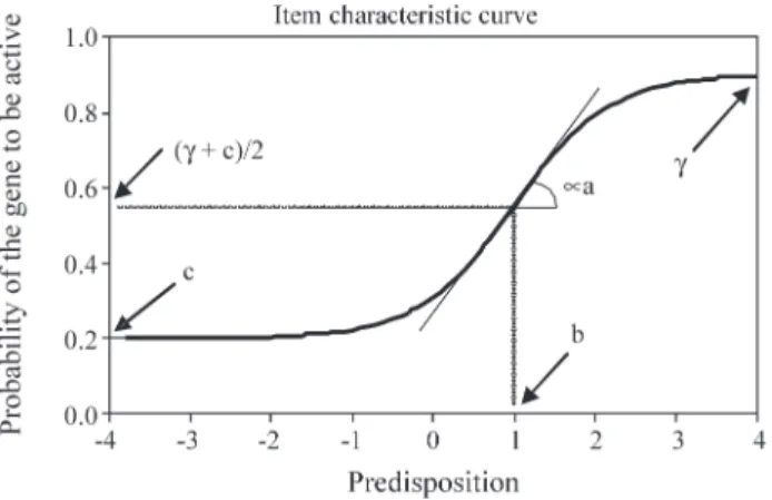
In a general way, the proposed model is based upon the fact that predisposed individuals are more likely to have the geneiactivated, and that this relation is not linear. As a matter of fact, it can be perceived from Figure 1 that the IRF has the form of “S” with inclination and displacement de-fined by the gene parameters. However, only a subset of genes has to satisfy this situation that occurs only when
ai> 0. Chances are that some genes are deactivated in high
propensity individuals, and therefore the IRF curve should
have an inverted form, expressing that individuals with high propensity are less likely to get the gene activated, and this is expressed byai < 0. When ai= 0, we have that
P U( ijk=1θ ζ, i) (= ci +γi) /2, constant for allθ, indicating
that the geneidoes not interfere in the occurrence of the anomaly.
Parameterbiis, perhaps, the most important of the
four. The greater this parameter is, less likely it is that a given individual has the geneiactivated. This is a valid conclusion only forai> 0, and the opposite is true forai< 0.
It is safe to say that individuals with low predisposi-tion are prone to have the geneiactive, and this information is conveyed by the parameterci. On the other hand, high
predisposition individuals can also have the geneiinactive, and this information is conveyed by 1 -γi. These
conclu-sions are valid only forai> 0, and the opposite is valid for
ai< 0.
Scale of Measurement/Indetermination
Predisposition can theoretically take any real value between -∞e +∞. Thus, it is necessary to establish an origin and a unit of measurement for defining the scale. When only one population is under study the scale of measure-ment can be defined in such a way as to represent the mean value and the standard deviation of the individual predispo-sitions of the population under study. For the graphs shown earlier the scale used had a mean of 0 and a standard devia-tion of 1, that will be referred from now on as scale (0,1). In practice, it does not make any difference to set these or any other values. What is paramount are the existent order rela-tions between scale points. For example, in the scale used above an individual with a predisposition of 1.2 in fact is 1.2 standard deviations above the predisposition mean. This same individual would have a predisposition of 92, and therefore would also be 1,2 standard deviations above the predisposition mean, if the scale used for this popula-tion would have been the scale (80,10).
When various populations are present, one of them can be adopted as aReference Population, and only the scale for this population will have to be refereed. The ob-tained predisposition values for other populations will have to be directly compared with those of the Reference Popu-lation. One such example consists of taking healthy indi-viduals in the Reference Population and the population with a certain anomaly as the other. Other populations can be taken into account.
Local Independence
this fashion it does not mean that the quantitiesUkjieUkjl,i≠
l, are independent, but given the individual predisposition
θjk they will be considered conditionally independent.
However, there are models for the case when conditional independence is not met, but we have to model this possible dependence.
Parameter Estimation of the Genes and
Predispositions
One of the most important stages of the IRT is the pa-rameter estimation of the genes and/or of the individual predispositions. In some cases we can consider that the pa-rameters of the genes are already known and what is wanted is to estimate the predispositions; in other, less common, predispositions of the individuals are known and what is wanted is the estimation of the parameter of the genes. However,the most common cases are those in which not only the parameters of the genes are to be estimated but
also the individual predisposition simultaneously. In all
these cases, the proposed model is assumed as true, and from the set of responses obtained for a certain number of individuals from one or more populations, parameters and/or predispositions are estimated using either likelihood or Bayesian methods. Both methods require iterative proce-dures involving very complex calculations and, therefore, specific computer codes. It is important to point out that, in any of these cases, the predisposition values and those of the gene parameters will all be in the same scale of mea-surement and therefore they can be compared.
Before outlining some points about the estimation process, some arrangements are in order. The set of genes involved in the analysis will be ordered in a fashion such that they will be represented by ζ = (ζ1,..., ζn). Let
Ukj. = (Ukj1, Ukj2,..., Ukjn) be a random vector of answers
from individualjfrom groupk;Uk..= (Uk1.,Uk2.,...,Ukn.) the
random vector of answers from group kand U... = (U1..,
U2..,...,Uk..) the whole vector of answers. In a similar
fash-ion, observed answers will be represented byukji,ukj.,uk.. andu.... This notation and local independence allow us to write the probability associated with the vector of answers
Ukjas
P ukj kj P u
i l
kji kj
k
( .θ ζ, )= ( θ ζ, ι) ∈
∏
(2)Generally, it is considered that the predispositions of the individuals of populationk,θjk,j= 1,...,Nk, are
accom-plishments of a random variableθk, with continuous
distri-bution and probability density function g(θ ηk), twice
differentiable, with the components ofηkfinite. In the case
whereθkhas a Normal distribution, we haveηk =(µ σk, k)
2
, whereµkis the mean andσk
2
the variance of the predisposi-tions of the individuals of the populationk,k= 1,...,K. This hypothesis carries a great advantage: only the parameters of
the genes have to be estimated, as the likelihood will not de-pend on the individuals’ predispositions. Therefore, the es-timation is a two-stage process, where in the first only the parameters of the genes are estimated, after which these pa-rameters are considered as known for the estimation of the predispositions.
Estimation of Gene Parameters
With the above defined notations we have determined that the marginal probability ofUkjis given by
P u P u g d
P u g
kj k kj k k
kj
( , ) ( , , ) ( )
( , ) (
. .
.
ς η θ ς η θη θ θ ζ
= =
ℜ
ℜ
∫
∫
θηk)dθwhere in the last inequality we use that the distribution of
Ukj.is not a function of parametersηk.
Utilizing the independence between answers of dif-ferent individuals, we can see that the associated probabili-ties to the vector of answersU...as
P u k P u
j N
k K
kj k
k
( ...ζ η, )= ( .ζ η, ) =
=
∏
∏
1 1
Even though the likelihood can be written as (2), the approach has often been used ofResponse Patterns. As we havengenes, with two possible answers for each item (0 or 1), there areS= 2npossible response vectors (response pat-terns). Letrkjbe the number of distinct occurrences of the
answer patternjin groupk, and yetSk≤min(Nk,S) the
num-ber of response patterns withrkj> 0. It follows that
rkj Nk j
Sk =
=
∑
1
By the independence between the answers of differ-ent individuals, we have that the data follows a
Product-Multinomialdistribution, that is,
(
)
[
]
L N
r
P u k
jk j
S kj k
j
S r
k k
k jk
( , ) !
!
,
.
ζ η = ζ η
= =
=
∏
∏
1 1
1
K
∏
And, therefore, the log-likelihood is
log ( , ) log !
!
log
L N
r
r
k
jk j S k
K
jk j
k ζ η =
+
= =
=
∏
∑
1 1
(
)
1 1
S
k K
kj k
k
P u
∑
∑
=
.ζ η,
(3)
The estimation equations for the item parameters are given by
∂ ζ η ∂ζ
log ( , )L
i
=0, i= 1,...,n,
(
)
∂ ζ η ∂ζ
∂
∂ζ ζ η
log ( , )
log . ,
L
r P u
i i jk j S k K kj k k = = =
∑
∑
1 1(
)
(
)
= = − = =∑
∑
r P u P ur u P
jk kj k kj k i j S k K jk kji i k 1 1 1 . . , , ( ζ η
∂ ζ η ∂ζ ) ( ) , * P Q P g d
i i i
j S k K kj k ∂
∂ζ θ θ ℜ = =
∑
∫
∑
1 1 whereg g u P u g
P u
kj kj k
kj k kj k * . . . ( ) ( , , ) ( , ) ( ) ( , )
θ θ ζ η θ ζ θη ζ η
≡ =
andPirepresents the IRF adopted. The specific equations
for each parameter of the vectorζi= (ai,bi,ci,γi)’ can thus
be obtained from above.
Application to the 4-parameter Logistic Model
For convenience, let
W P Q
P Q i i i i i = * * (4)
wherePi
{
e}
Dai bi
* = + − ( − ) −
1 θ 1andQi*= 1 -Pi*.
In sum, the estimation equations forai,bi,ciand γi
are, respectively,
D ci rkj ukji Pi b W gi i d
j S k K kj k
(1 ) ( )( ) * ( )
1 1 − − − = ℜ = =
∑
∫
∑
θ θ θ 01 0 1 1 , ( ) ( ) * ( ) − − − = ℜ = =
∑
∫
∑
Dai ci rkj ukji P W gi i d
j S k K kj k
θ θ ,
( ) ( ) ,
(
* *
r u P W
P g d
r u
kj kji i
i i j S k K kj kj kj k − = ℜ = =
∑
∫
∑
1 1 0 θ θ i i i i j S k K kj P WQ g d
k − = ℜ = =
∑
∫
∑
) * * ( ) , 1 1 0 θ θwhich do not have explicit solutions. Therefore, such esti-mations are arrived at by iterative processes, such as New-ton-Raphson, BFGS, Fisher’s Scoring or EM algorithm.
Estimation of the Population Parameters
Considering the log-likelihood obtained in (3), the es-timation equations for the mean predispositions and popu-lation variances are obtained by
∂ ζ η ∂µ
log ( , )L
k
=0
and
∂ ζ η ∂σ
log ( , )L
k
2 =0
k= 1,...,K. However,
∂ ζ η ∂η
∂ θη
∂η θ θ
log ( , ) log ( )
( )
*
L
r g g d
k kj k k kj j = ℜ
∫
=∑
1 Sk .If we use the distributionN(µk,σk2) forθk, we have
∂ θη ∂µ
θ µ σ
log (g k)
k
k
k
= −2
and
∂ θη ∂σ
σ θ µ σ
log (g k) ( )
k k k k 2 2 2 4 2 = − −
Thus, the final forms of the estimation equations for
µkandσk2are, respectively,
( )
(
)
( )
(
)
σ θ µ θ θ
σ σ θ µ
k kj k kj
j S
k kj k k
r g d
r
k
2 1
1
4 1 2
0 2 − ℜ = − − = − − −
∫
∑
* ( ) ,[
2]
1
0
gkj d
j Sk
*
( )θ θ . ℜ
=
∫
∑
=Estimation of the Predispositions
Once the parameters of the genes are set, individual predispositions can be estimated. In addition, such predis-positions can also be estimated for individuals whose data were not considered in the item parameters estimation. The usual methods for estimating the predispositions are the maximum likelihood (ML) as well as Bayesian methods such asmaximum a posteriori (MAP)and theexpected a
posteriori (EAP).
Estimation by ML
In this case, the estimation of the predispositions is done iteratively by the Newton-Raphson algorithm maxi-mizing the likelihood in (2), or of the equivalent form, the function
(
)
{
}
log ( )L ukjilogPkji ukji logQkji i n j S k K k
θ = + −
= = =
∑
∑
∑
1 1 1 1The Maximum Likelihood Estimator (MLE) ofθkjis
that which maximizes the likelihood, or equivalently, is the solution of the equation
∂ θ ∂θ
log ( )L
kj
=0,j= 1,...,Nk,k= 1,...,K. (5)
∂ θ ∂θ
∂ ∂θ
∂
log ( ) (log )
( ) (log )
L
u P u Q
kj kji kji kj kji kji
= + −1
∂θ ∂ kj i n kji kji kji kji kji u
P u Q
P = − − =
∑
1 1 1 1 ( ) ∂θ ∂ ∂θ kj i n kji kji kji kji kji kj u P P Q P = − =∑
1 = − =∑
i n kji kji kji kji kji kji kju P W
P Q P 1 ( ) * * ∂ ∂θ =
∑
i n 1 (6)where the last equality follows by (4), and when plugged in the respective quantities. As
∂ ∂θ
P
Da c P Q
kji
kj
i i kji kji
= ( − ) * * , 1
it is obtained
h kj L D a c u P W
kj
i i kji kji kji
i n
(θ ) ∂log ( )θ ( )( )
∂θ
≡ = − −
=
∑
11
It follows then that the estimation Eq. (5) for θkj,
j= 1,...,Nk, is
D ai ci ukji Pkji Wkji
i n
(1 )( ) 0.
1
− − =
=
∑
Again, this equation does not have an explicit solu-tion forθkjand, for this reason it is necessary for some
itera-tive method in order to obtain the desired estimation. Following, the necessary expressions are obtained for ap-plications of the Newton-Raphson iterative processes.
Consideringθ$( )
kj t
an estimation of θkj in iteration t,
then, in iterationt+ 1 we have
( )
[
]
( )
$( ) $( ) $( ) $( ) ,
θkj θ θ θ
t kj t kj t kj t H h
+1 = − −1
where
( )
[
]
H kj ukji P Wkji kji Hkji ukji P W hkji kji kji
i n
θ = − × − −
=
( ) ( ) 2
1
∑
with
(
)
hkji P Qkji kji Pkji Da c
kj i i = = − −
* * 1 ∂ (1 )
∂θ (7)
and
(
)
Hkji P Qkji kji Pkji D a c P
kj i i = = − − −
* * 1 ( )(
2
2
2 2 1 1
∂
∂θ kji
*) (8)
Estimation by MAP
Such as in the marginal likelihood estimation, the Bayesian estimation of the predispositions is done on the second stage, considering the fixed parameters of the genes. Through the hypothesis of independence between
the predispositions of different individuals, estimations can be done separately for each individual.
Let us assume that the prior distribution for θkj,
j= 1,...,Nk, is Normal with known vectorηk =(µ σk, k)
2
of parameters. The posterior distribution for the ability of the individualjof the populationkcan be written as
gkj kj g kjukj P ukj kj g kj k
*
. .
(θ )≡ (θ , , )ς η ∝ ( θ ς, ) (θ η ) (9) Some characteristic of gkj kj
*
(θ )can be adopted as es-timator ofθkj, where the most frequently adopted are the
mean and the mode. Following, we deal with how to obtain each of these characteristics.
Estimation of the mode of the posterior distribution -MAP
The Bayesian modal estimation consists in obtaining the maximum of (9). For easiness, we work with the loga-rithm of the posteriori
logg*kj(θkj)= +C logP u( kj.θ ςkj, ) log (+ g θ ηkj k), whereCis a constant. It follows that the estimation equa-tion forθkjis
log ( ) log ( , )
log ( )
*
.
g P u
g kj kj kj kj kj kj kj k θ ∂θ
∂ θ ς ∂θ ∂ θ η
= +
∂θkj
=0
(10)
By local independence, we have that
log ( , ) log ( )
log (
.
P u P u
P u
kj kj kji i kj
i n
θ ς = ς , θ = =
∏
1kji i kj i
n
ς , θ ). =
∑
1
Therefore,
∂ θ ς ∂θ
∂ ς , θ ∂θ ∂
logP u( . , ) logP u( )
P kj kj
kj
kji i kj
kj i n = = =
∑
1 ( ) ( ). u P ukji i kj
kji i kj i
n ς , θ
ς , θ
=
∑
1
Keeping in mind thatP ukji i kj Pkji Q u
kji u
kji kji
( ς θ, )= 1− and
using the development under (5), we have that
∂ θ ς ∂θ
log ( , )
( )( )
.
P u
D a c u P W
kj kj
kj
i i kji kji kji
i n = − − =
∑
1 1 (11)As we have adopted the prior distribution Normal (µk,
∂ θ η ∂θ
θ µ σ
log (g kj k) ( )
kj
kj k
k
= − −2
By (11) and (12), we have that the estimation equa-tion forθkjis
D ai ci ukji Pkji Wkji
kj k
k
(1− )( − ) −( −2 )=0.
∑
θ σ µAs this equation does not have an explicit solution, some iterative method can be used to solve it. To do that it is necessary the second derivative of log * ( )
gkj θkj with
rela-tion toθkj, whose expression is
( )
H u P W
H u P W h
kj kji kji kji
i n
kji kji kji kji kji
θ = − ×
− −
=
∑
( )( )
1
[
2]
2
1
− σk
,
wherehkji andHkjiare given by (7) and (8), respectively.
Estimation by EAP
The Bayes expected a posteriori (EAP) consists in ob-taining the expectation of the posterior distribution, that can be written as
g u P u g
P u
kj k
kj k
kj k
( ) ( , ) ( )
( )
.
.
.
θ , ς, η θ ς θη ς,η =
It follows that the estimator is given by
[
]
$ ( ) ( )
( ) (
.
.
.
θ θ , ς, η θ θη θ, ς θ θη
kj kj k
k kj
k kj
E u g P u d
g P u
≡ =
∫
ℜθ, ς θ)d
ℜ
∫
This form of estimation has the advantage of being calculated directly, not being necessary the application of iterative methods.
Simulation Results
In this section we present one application of the pro-posed methodology in simulated data. The data were gener-ated based on N = 5000 individuals and ton= 5 genes. The total simulation consisted of 1000 replications. The known gene parameters are presented below. All the calculations were done via a computer program developed by the au-thors using the computer languageOx(see Doornik, 1998) using the BFGS routine for maximization.
The Genes Parameters
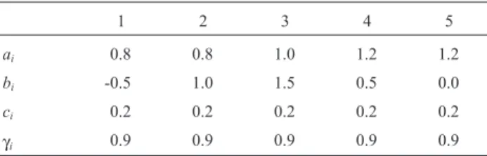
In order to generate the data it was assumed that the genes parameters are those presented in Table 1. It was adopted the 4 parameter logistic model with D = 1.7. The values for parameter a (discrimination) varied from 0.8 (low discrimination) to 1.2 (high discrimination) and the values for parametersb(predisposition) varied from -0.5 to
3.0. For the parameterscit was considered only one value (0.20) and for theγ, only 0.9. It was adopted the 4 parameter logistic model withD= 1.7.
From Table 2 we see that the average estimates ob-tained from 1000 replicates are very accurate for all genes. We see that the estimations procedure works very well, still when we have a relatively small number of genes. Results were obtained with a larger number of genes and the results were still very good. However, we hope that estimation problems just appear when the number of genes is too small.
The Table 3 presents the standard deviations obtained from 1000 estimates. The largest values are associated with the parametersaandb. With exception of the gene 2, the values associated with parameteraare larger than those as-sociated tob.
Concluding remarks
We have introduced a new proposal for genes and person diagnostic via Item Response Models. From a simu-lation study, it was shown that the models provide good es-timates for several genes configurations. However, other studies and models should be proposed to allow, for exam-ple, different levels of activities of the genes. Longitudinal models, following the lines of Tavares and Andrade (2004) and Andrade and Tavares (2004), should also be consid-ered.
Table 2- Deviations from the average estimates with relation to the true gene parameters.
1 2 3 4 5
ai 0.0193 0.0333 0.0233 0.0254 0.0117
bi 0.0021 -0.0103 0.0472 -0.0062 0.0038
ci -0.0038 -0.0038 -0.0036 0.0001 -0.0006
γi 0.0042 0.0031 0.0195 -0.0031 0.0020
Table 1- Genes parameters.
1 2 3 4 5
ai 0.8 0.8 1.0 1.2 1.2
bi -0.5 1.0 1.5 0.5 0.0
ci 0.2 0.2 0.2 0.2 0.2
γi 0.9 0.9 0.9 0.9 0.9
Table 3- Standard deviations for the 1000 estimates.
1 2 3 4 5
ai 0.1576 0.1738 0.2562 0.1293 0.1164
bi 0.1080 0.2055 0.2019 0.0934 0.0804
ci 0.0346 0.0377 0.0244 0.0242 0.0232
Acknowledgments
This work was partially supported by grants from Conselho Nacional de Desenvolvimento Científico e Tec-nológico (CNPq), Coordenadoria para o Aperfeiçoamento de Pessoal de Nível Superior (CAPES), National Program of Excellency (PRONEX) contract No 76.97.1081.00, The-matic Project of Fundação de Amparo à Pesquisa do Estado de São Paulo (FAPESP) contract No 96/01741-7, Inte-grated Program for Teaching, Research and Extension (PROINT) of the UFPA, and PARD. It was partially devel-oped when the first author was a doctoral student at the De-partment of Statistics of the University of São Paulo.
References
Andrade DF and Tavares HR (2004) Item response theory for lon-gitudinal data: Population parameter estimation. To appear in Journal of Multivariate Analysis.
Andrade DF, Tavares HR and Valle RC (2000) Item Response Theory: Concepts and applications. Associação Brasileira de Estatística, São Paulo (in Portuguese).
Bock RD and Zimowski MF (1997) Multiple Group IRT. In: van der Linder WJ and Hambleton RK (eds) Handbook of Mod-ern Item Response Theory. Spring-Verlag, New York. Chow YS and Teicher H (1978) Probability Theory:
Independ-ence, Interchangeability, Martingales. Springer-Verlag, New York.
Doornik JA (1998) Object-Oriented Matrix Programming using Ox 2.0. Timberlake Consultants Ltd and Oxford, London. www.nuff.ox.ac.uk/Users/Doornik.
Hambleton RK, Swaminathan H and Rogers HJ (1991) Funda-mentals of Item Response Theory. Sage Publications, New-burg Park.
Lord FM (1980) Applications of Item Response Theory to Practi-cal Testing Problems. Lawrence Erlbaum Associates, Inc., Hillsdale.
Paas LJ (1998) Mokken scaling characteristic sets and acquisition patterns of durable and financial products. Journal of Eco-nomic Psychology 19:353-376.
Tavares HR and Andrade DF (2004) Item response theory for lon-gitudinal data: Item and population ability parameters esti-mation (to appear in Test).