A Work Project, presented as part of the requirements for the Award of a Masters Degree in Finance from the Faculdade de Economia da Universidade Nova de Lisboa.
THE HIDDEN VALUE BEHIND CAPITAL STRUCTURE DECISIONS
CARLOS AFONSO BI FRANÇA E SILVA
Nr. 175
A Project carried out on the financial area, with the supervision of:
Professor Pedro Santa-Clara
2009, June
2
ABSTRACT
I estimate the optimal capital structure for a growth company, for which market value is
dictated by its highly volatile nature. I study the welfare impact of corporate taxes,
analyzing their economic effect of inducing higher bankruptcy levels. Assuming that
management always seeks to optimize the market value of company’s assets, I find a
significant loss of value that varies negatively with volatility. Flow and stock insolvency are
important for the maximization of capital structure, and I compare both, modeling the
value of the company as an option on its revenues. These are not only highly significant for
R&D and startup companies but also have significant welfare consequences. I compare the
options of liquidation and re-financing and find a clearly important role of early liquidation
for R&D frameworks. I complement the study with a comparative statics analysis
estimating the impact of risk to the value of the firm and the optimal capital structure
decision, for a cross-section of firms. The results present quantitative evidence that
reinforce the literature of trade-off and capital structure applied to growth companies.
Keywords: Capital Structure, Real Options, R&D valuation, Simulation.
INTRODUCTION
We know a lot about what conditions capital structure decisions, but not much about either
how to estimate accurately the real value-maximizing level of debt for a specific firm, or
how to estimate the impact of these decisions for the whole economy. While there is an
3 balancing tax advantages against bankruptcy costs is consensually accepted in the
profession as a significant aspect to be taken into account. Decisions based upon this
premise may nevertheless lead to a perverse social effect. Corporate taxes impose a
distortion on economy by giving managers the incentive to choose higher leverage
structures. I will show that as a direct consequence of this, the number of bankruptcies
increase leading to a market inefficiency, as part of the firm’s value can be appropriated by
neither government, nor debt/stock-holders and is therefore lost. This paper explores
these two concepts. I propose a valuation framework1 for the estimation of optimal debt
levels and use the results to deduce the impact of taxes on social welfare resulting from
bankruptcy levels.
The capital structure decision, key to every company, assumes a particularly interesting role
for R&D or startup companies exhibiting high operational volatility. There is empirical
evidence of R&D managerial preference for conservative levels of debt (Long and Malitz
(1985), Long and Malitz (1983), Myers (1977), etc.). A proposed explanation2 for this
conservativism is the presence of costs3 other than bankruptcy, varying positively with debt
ratios, impacting such firms to a wider extent than they do for value stocks. Amongst other
contributions that extend the bankruptcy costs, under-investment is of most importance to
R&D (for instance Myers4 (1977)). Growth companies that by definition have their value
linked to cash-flows deferred to the future are heavily dependent on ensuring the
1 I explore the extensive empirical research on capital structure in appendix I, and find that most tests focus on proving a relation between debt ratios and a multitude of factors (volatility, growth options, size, etc), but there are not as many contributions towards measuring these relationships.
2 Other explanations include the need to control agency costs of debt, that can only be done through limiting debt outstanding, since the effectiveness of bond covenants is reduced if a firm’s value is strongly based on intangible growth options (Long and Malitz (1983)); (O’Brien (2003)) points out both the necessity to keep a steady flow of cash for R&D windows of opportunity and product market introduction (financial slack).
3 The cost of under-investment is described for example in Myers (1977).
4 availability of funds to carry-out their growth and investment options. Myers builds on this
notion to include the cost of under-investment, for which management will rationally
follow a different decision path than they would for an unlevered investment (or riskless
debt) and will tend to pass up positive opportunities, investing only when the expected gain
is higher than the promised payment to bond-holders.
To fully capture the impact of these intrinsic R&D costs and the value of management
decisions5 for highly volatile investments, different valuation techniques besides the
traditional discounted cash-flow approach must be used. Traditional techniques value
investments in one step accounting neither the importance of flexibility on investment
decisions nor the possibility of risk changing over the course of the project. I believe that
the study of R&D companies is pointless if such features are not captured6.
I propose the use of a framework that allows the liquidation of the company based on its
market value (stock distress), at each period, long before the project takes a negative turn
with debt-holders taking possession of company’s assets (flow distress). I do this by
modeling the firm’s value as an American call option on the firm’s revenue (that in turn
follow a stochastic process with time-varying volatility).
Research is vast in models for company valuation and capital structure (nevertheless,
contributions to the latter, model mostly flow distress, choosing to invest until firm’s assets
reach zero, regardless of its economic value). Previous studies in this area that have
developed concepts relevant to this paper include Schwartz and Moon(2001) and Schwartz
and Gorostiza (2000b) that take into account stock distress utilizing an option theory
framework similar to the one I apply; Strebulaev (2007) estimates the optimal capital
structure maximizing the value of the company at time zero, allowing for costly
5 financing in liquidity stress which is also included in my contribution; Goldstein, Ju and
Leland (2001) model the cash flows as a geometric Brownian motion and solve for the
optimal coupon and bankruptcy level allowing for debt levels to change through time; Miao
(2005) models the level of technology idiosyncratic shocks (innovation level) and chooses
to invest while above a certain threshold7, but does so using an equilibrium model not
suitable for an individual firm calculation and therefore difficult to apply in this case.
I adapt the model derived by Schwartz and Moon (2000)8 in which risk takes the central
role, adding capital structure features such as in Strebulaev (2007). Schwartz and Moon
developed this model to value Internet companies and make sense of the irrational
exuberance of stock prices9 prior to the dot.com crisis. They model stochastic revenues
highlighting volatility in its several forms10 to a much larger extent than other authors,
which is important if we expect the option value to hold a significant share of the firm’s
value.
There is a multitude of factors influencing capital structure decisions, but the most decisive
can be classified into two main families11: the Trade-Off between taxes and several costs
(bankruptcy, agency, under/over-investment, etc.) or the Information Asymmetry theories
(market timing, pecking order and signaling). The Trade-Off concept is the basis of this
paper as it not only has an important economic reasoning when applied to R&D valuation
but is also easy to model in simulation.
7 He chose this setup up to capture the under-investment problem in Myers (1977).
8 The original model is disregards capital structure; I introduce it and include the cost of re-financing under liquidity stress.
9 A reference to Shiller’s book that forecasted the dot.com crash. A lot of literature was developed in the late 90’s by researchers and practitioners making use of real options to explain the difference in valuation found by DCF approaches and observed market prices.
10 They model high (stochastic) time-varying expected rates of growth and unanticipated time-varying shocks to the expected rate of growth.
6 Based on the results of the simulation framework that models the company operations as
an American real option on the revenues, with capital structure decisions, I will measure
the perverse social welfare impact of taxes and perform a comparative statics analysis to
capture the impact of risk to financing decisions for a cross-section of firms in order to
demonstrate the impact of capital structure decisions both from the viewpoint of rational
management and governmental taxation policy makers.
The rest of the paper is organized as follows, section 2 presents details of the model, data,
simulation methods and assumptions. Section 3 analyses the findings and valuation, using
amazon.com to calibrate the model. Here are included sub-sections for flow and
economical distress, comparative statics and welfare analysis. Section 4 analyses the results
and summarizes the conclusions. Lastly the appendix reviews the capital structure
literature, classifying the vast contributions (from 1958 to 2008) to capital structure
including empirical evidences into a survey that I very modestly attempt at.
THE MODEL
To value a company that holds significant growth options, some stylized facts are of crucial
importance. First, volatility is what drives value. Therefore, revenues are modeled using a
geometric brownian motion but accounting not only the volatility in revenues but also
making the drift stochastic (and time-varying) and bringing unanticipated changes of the
drift into the equation12. Second, startup companies exhibit extremely high volatility and
growth rates when they initiate operations, but converge after a period to average industry
values. In the model, these processes are made mean-reverting to capture this feature.
7 Lastly, the model is developed assuming a limited liability company and for simplicity, a
time horizon after which the company terminates operations and distributes the remaining
cash-flow to share-holders.
To solve for the optimal capital structure I maximize the company value at time zero by
simulation, for several debt levels13. According to the trade-off theory, the total value will
be given by the sum of the equity-holder value, debt-holder value and taxes.
(1)
While the total value will remain constant14, management will rationally choose to increase
the share available to investors at the expense of taxes. Specifically, managers will choose to
optimize the first two components on the right side of equation (1).
The value of the equity is the present value15 of the assets ( ) remaining at the end of the
firm’s life (time T). The dynamics of the assets evolve, by accumulating net income, as all
earnings are retained in the company until the horizon to avoid complicating the model
with a dividend policy.
(2)
(3)
The value of debt in time zero is the sum of the present value of all debt payments (DP).
As DP is constant, the value depends only on the liquidation or bankruptcy of the
company.
(4)
13 To find an accurate debt level I developed a maximization algorithm that iteratively decides for a direction of search and divides value-debt_level curve in half towards a neighbor known point.
14 The value remains constant for the same amount of bankruptcies. Increasing debt levels will increase the number of bankruptcies and therefore will reduce the total value.
8 The present value of taxes (TX) is given by equation (5). T can be either the horizon or the
period when bankruptcy (flow or stock) happen.
(5)
The net income ( ) is calculated from equation (6)-(11), where DP is the debt payment
and the tax expense in period t. Taxes are only paid if the loss carry forward ( )
equals zero. Its dynamics are given by equation (8).
(6)
(7)
(8)
is the revenue at time t, COGS the cost of goods sold and SGA the selling, general and
administrative expenses. COGS is proportional16 to the revenues and SGA has both a
proportional part of variable costs and a fixed cost FC constant in time. These parameters
were estimated in Schwartz and Moon (2000) and are shown in table 3 in the appendix.
(9)
(10)
(11)
There are two sources of uncertainty in this model both incorporated in the revenues
which follow the geometric Brownian motion of equation (12).
(12)
The stochastic equation captures the high uncertainty of an R&D or startup company.
Both the drift and the volatility are time-varying. The drift has been adjusted downwards
9 with the market price of risk ( ) so that valuation in equations (2), (4) and (5) can be done
using the risk-free rate using the adjusted expectation operator.
The drift is given by equation (13). It is a mean reverting process, also risk adjusted by ( ),
modeling an initial high expected rate of return that with time falls to a more conservative
level. The unanticipated change in the growth rate of revenues is given deterministically by
the zero-reverting equation (14).
(13)
(14)
The volatility in the revenues is given by the deterministic mean reverting equation (15).
(15)
Both volatility parameters start high but volatility in revenues converges to a lower value
while shocks to the rate of growth of revenues disappear as the company matures.
Cash varies with each period’s net income17, until either it is exhausted and reaches zero or
a decision of liquidation is made, based on the market value of the company. When assets
are exhausted bankruptcy happens and is accounted to the calculation of default
probability. At each period the value of future cash-flows is forecasted using the Longstaff
and Schwartz18 (2001) method. Forecasting the market value models the management
decision to liquidate or continue in operation. The case when the company continues to
operate and cash is below zero, models a creditors protection in which the company can
negotiate and eventually leave the troubled situation, evolving towards positive grounds. To
avoid that the model allows the company to stay in operation despite very negative results,
17 To make share-holders indifferent to when they receive the company cash-flows and therefore avoid defining a dividend policy, assets compound each period at the risk-free rate.
10 I introduce a parameter to emulate the increased difficulty in raising new financing
(therefore forcing stock distress sooner than would otherwise occur).
Some simplifications are obvious from the equations. First, the model has no investment
decisions and no CAPEX. An investment policy would be interesting to add to the
framework, especially accounting the role of innovation. Several studies that use Poisson
draws to model the discovery of ideas would be easily adapted to bring more realism into
the setup of real options (Schwartz and Gorostiza (2000a), Schwartz and Gorostiza
(2000b), Schwartz (2004), etc.).
Second, depreciation tax shield was not included in the model, even though it would also
be easy to do. Depreciation would nevertheless complicate the analysis of the tax effects to
debt level (contributions that could be used are Schwartz and Moon (2001)).
Third, costs: variable costs are a constant percentage of revenues, imposing a deterministic
effect in EBIT in each period. This feature does not account for a learning curve that is
part of every company. More importantly, fixed costs stay constant throughout time,
eventually leading to an underestimation of bankruptcies in the model. Catastrophic events
are also important for the value of these companies (e.g. competition and technology
shocks). There is a significant amount of contributions that make use of Poisson variables
to include negative value-destroying jumps ((Pyndick (1993), etc.).
Fourth, interactions with other companies would be interesting to model in order to
capture a company much dependant on a single product, and thus largely impacted by
competitor’s actions. A recent area, that mixes real options with game theory to value R&D
companies has given interesting contributions for a case such as this one (e.g. Miltersen and
Schwartz (2004)).
Lastly, debt payments are kept constant throughout the lifetime of the firm. The most
11 target debt ratios (Leary and Roberts (2005) and Hovakimian and Opler and Titman
(2001)).
The reason not to model all these features was the trade-off between realism and simplicity.
While the inclusion of some of those would not be difficult to achieve, it would complicate
the analysis and deviate the attention from the debt-equity choice focus.
Data used to calibrate the model is reported in appendix III. All values, including some that
are used to compare simulation results are based on published financial information from
Bloomberg and amazon.com’s financial statements reported until the 3rd
quarter of 1999
(the same data utilized in the Schwartz and Moon (2000)). Amazon.com is an iconic
example of the .com era. Heavily biased towards growth, amazon exhibits a p/e ratio of 78
and is heavily dependent on its innovation capabilities (it invests 9.9% of its total sales in
R&D expenditures). What may appear at first a simple business model is in fact a
multi-level e-commerce platform based on state-of-art patented algorithms for recommendation
and customer tracking.
RESULTS
I. Basic Results
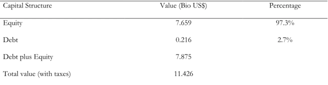
The optimal estimated capital structure for amazon.com is reported in table 1 along with
the corresponding debt-to-value and equity-to-value ratios. The model estimates
significantly conservative levels of debt, in line with the empirical evidence for growth
companies. (Myers (2001)) reports debt levels for different industries, examplifying the case
of pharmaceutical companies typycally operating at negative debt ratios19, besides the
12 overly quoted case of Microsoft. Notice that amazon exhibits a large default probability of
35.7% (stock distress is 36.6%) after optimizing the debt level, from an already high
starting all-equity probability of 30.5% (33.4% stock distress). It is not surprising that
amazon was already near its debt capacity before the optimization.
The value of amazon for each level of fixed debt payment is reported in figure 1. The
optimal debt has an expected value of 0.216 billion US$ and implies fixed responsibilities
of 6 million US$/quarter20.
Figure 1: Optimal Debt Values. The debt payment levels that maximize debt, from the perspective of Debt plus Equity.
20 Amazon has at time zero revenues of 906 million US$ per quarter and variable costs that amount to 94% of sales, leaving a profit margin of 6%.
Capital Structure Value (Bio US$) Percentage
Equity 7.659 97.3%
Debt 0.216 2.7%
Debt plus Equity 7.875
Total value (with taxes) 11.426
13
II. Flow Distress, Probability of bankruptcy
Valuation under different capital structures has to account the increasing probability of
default (either flow or stock) that offsets the increase in value by means of tax shield. As
the probability of default increases, the expected cost of bankruptcy21 also increases thus
reducing the overall expected value of the firm. This might prove unberable to most
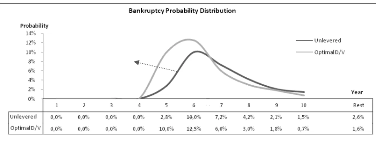
investors holding claims on the company cashflows. The bankruptcy distribution is
reported in figure 2 for the unlevered and optimal structures of capital.
For all simulated scenarios, default occurs in the first years of operation when the initial
cash balances are exausted. Increasing debt levels shifts default towards the beginning of
the operations at the same time as it increases overall probability. In the not reported cases
of extremelly high debt, bankruptcy happens 100% of the times in the first period. If the
company survives the first years of operation, bankruptcy probability falls to insignificant
values (after year 10 is less than 3%).
Figure 2: Bankruptcy Probability Distribution.
This feature models the extremely high uncertainty of a venture such as amazon in its initial
years, as it goes trhough an affirmation period. During this period its revenues are highly
14 volatile and its fixed costs play a crucial role for its survival. After the first initial years, if
cash balances are not exhausted by strongly negative results, the fixed costs that push
bankruptcy scenarios in the first years will become less significant22. In the long run the rate
of growth of sales will diminish, its volatility will tend to zero, as the company reaches
maturity and solidifies its position in the market.
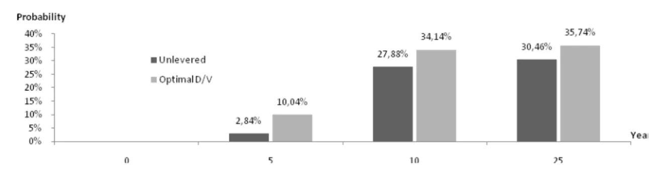
Figure 3 depicts another perspective of the bankruptcy probability, reporting accumulated
figures, where total results are easier to see. For the optimal scenario, default occurs
35.74% of the times.
Allowing the liquidation of the company before it falls in distress, even though augmenting
the number of bankruptcies, significantly increases the value for equity-holders as they do
not have to wait until cash is exhausted and debt-holders take posession of the company23.
This model always forces optimal bankruptcies, therefore solving the Management
Entrenchment problem24 that is found on numerous times in real cases. Management in
this scenario always acts in the best interest of share-holders.
If we allow in the model for the company to recover after failing to match payments
(entering a flow distress situation), introducing increased costs of re-financing, we reach
exactly the same conclusions. The value of this (waiting-for-a-recovery) option proved
insignificant in simulation. R&D companies are strongly affected by timing: failing the
window of opportunity to introduce a product in the market leads to severe loss of
competitiveness25 and devalue of the growth opportunities. While forecasting earlier the
22 This is modeled by the drift in the geometric brownian motion, making sales grow in the long run.
23 The value of the company is strongly dependant on the option value, which is to say that the value of ownership decision plays a significant role in the model.
24 Debt is issued in its optimal level (maximizing value), disregarding other considerations.
15 lack of economic viability increases significanty the value of the firm, letting the venture
continue, waiting for a recovery along the path is of much less interest for an R&D
company. Having small cash balances and lacking sellable assets, it typically enters a stage
in which death is innevitable.
Figure 3: Bankruptcy Probability Distribution Accumulated.
II. Welfare Analysis
Debt tax shield introduces an incentive for management to rationally increase debt levels.
This has the perverse effect of inducing a larger number of bankruptcies with consequent
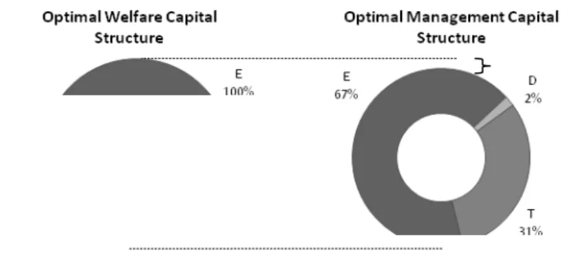
loss of value. This inefficiency is reported in figure 1, where the total value26 of amazon for
its optimal estimated debt level is compared to its estimated value under a no-tax setup
(thus with no incentive to have debt). The size of the charts captures the loss of value in
the scenario of 0.35 tax rate (the rightmost plot).
The estimated optimal value of the company would be 11.485 billion US$ for the no-tax
scenario and 11.426 billion (less 59 million) induced by a higher level of bankruptcies, from
33.4% (default probability) to 36.6% after debt-equity optimization. The introduction of
taxes leads to a destruction of 0.51% of total company value.
16
Figure 4: Optimal Capture Structure from the point of view of management, destroys value by inducing a higher number of bankruptcies.
Even for this conservative estimate of capital structure there is a significant effect of the
tax shield when looking from the perspective of the overall value for society. There is a
non negligible social loss to be considered by taxation policy makers. This value would
even be more extreme for companies exhibiting state variables less extreme as those of
amazon. For a company that started operations with less significant probability of default,
the effect of optimizing its capital structure by means of tax shield, would lead to a higher
change in default probability and thus to a more extreme destruction of value.
17 Figure 6 reports the comparative statics effect of tax shocks to the total value of amazon
and for its bankruptcy probability.
Figure 6: The effect of taxes for total value and default probability.
The right chart reports the value under each tax rate as a percentage of the value under the
no-tax scenario. There is a loss of 0.51% for the normal US tax rate and 0.67% when taxes
increase by 5%. In extreme (unreported) scenarios the drop becomes steeper and
eventually taxes alone become unbearable for a company to operate.
In the leftmost chart, bankruptcy levels increase positively and significantly with taxes,
explaining the loss of total value in the first chart.
III Comparative Statics
I analyze the effect of shocks in the parameters of the model, reporting the ones that
proved to be more significant in the simulation (variable costs and volatility). Their effect
on value (debt and equity), probability of bankruptcy and change in the optimal
debt-to-value ratio is discussed below.
18 The first and most obvious parameters that significantly influence the company are variable
costs. As the OLS-estimated variable costs ( and ) are assumed to remain constant
throughout the lifetime of the company, they have a stronger importance than their fixed
counterpart, as the latter while having the power of bankrupting the company in the first
years, soon becomes less relevant27. As would be expected, even a conservative change of
1% upwards or downwards, exerts a significant effect on the three analyzed aspects.
Optimizing the capital structure of the company for the new cost figures, the overall value
moves from 7.875 billion US$ to [6.364; 9.177]. Overall this represents a variation of -19%
in value when costs increase and 16% when costs drop. Debt-to-value varies between [2%;
4%], increasing the debt capacity of the company when costs drop. Bankruptcy also varies
positively with costs from 37% to [33%, 44%].
Figure 7: Comparative Statics, change in volatility and variable cost parameters.
19 Valuing any company is an exercise in which costs have to be carefully estimated. It
becomes apparent the role of management in driving costs down, trough a learning curve
as it may be the difference between success and bankruptcy (notice the high variation in
distress probability) as a 1% increase in costs lead to 19.5% increase in the probability of
default.
Volatility parameters
I test the effect of change in both the volatility of revenues (from 0.1 to 0.05 and 0.15) and
rate of growth of revenues (from 0.03 to 0.01 and 0.05). Their behavior is identical, but the
change in the rate of growth is far more extreme. Value changes from 7.875 billion US$ to
[7.813; 7.948] for the parameter and [4.040; 24.146] for . The volatility in the rate of
growth has the capacity of increasing value in 200% or decreasing it to 50% of its value.
Debt ratios vary from 2,7% to [1%; 6%] ] for and [2.6%; 3.3%] for . Bankruptcy
varies from [35%; 40%] for and [21%; 43%] for .
There is an important difference between the behavior of the two parameters. Volatility in
the revenue drives the value slightly down as it increases default in 3%, while the shock in
the rate of growth has the opposite effect (it doubles value). This is a finding in line with
the observation performed in Schwart and Moon (2000). While volatility in revenues drives
bankruptcy and therefore predicts lower debt-ratios28, less volatility lead to stable revenues
allowing for a higher debt capacity.
Volatility in the rate of growth has the opposite effect. It allows for extremely high (or low)
rates of growth and therefore it captures the value of the option (as positive paths lead to
large cash-flows and negative paths are liquidated early in the simulation). These are the
20 scenarios where the option exerts its value, and what would be expected from the intuition
of real options: the more volatility amazon has, the more valuable it will be. Volatility
parameters evolve according to: increases, so does distress, but value and D/V decrease;
increases, so does distress and value, but D/V decreases.
D U N
σ 3,3% 2,6% 2,7%
η 5,5% 0,8%
Cost 4,9% 2,0%
Table 2: Optimal Debt ratios for the perturbed parameters (U: upward change; D: downward change).
Welfare values can be directly inferred from the estimated bankruptcy values. For the
perturbed parameters, the value lost varies significantly solely for the shock on the volatility
in the rate of growth of revenues. In this case the loss varies between [0.18%; 1%]. Being
that the highest loss (1%) happens when drops in value. A conclusion can be drawn,
that the less volatile a company is (and the less valuable is the option) the higher will the
social loss be. This is explained by the bankruptcy values. For the increase in volatility there
is a probability of default of 43% for the optimized case compared to 40% for the no-tax.
In negative shock, the values are 21% compared to 17%. As the value for the no-tax
incorporates a very extreme probability driven by the high volatility values (not the debt
level), the change introduced by taxation is less extreme. When volatility is high, the effect
of taxes therefore is less extreme, as bankruptcies are already at a high level. Therefore the
loss of welfare is higher for more stable industries, for which debt capacity is higher and
21
CONCLUSIONS
The analysis of a growth company under a target static debt ratio, modeling the trade-off
between taxes and bankruptcy leads to important conclusions, for investors doing R&D
valuation, managers and governmental policy makers.
Social welfare is significantly affected by the way taxes are constructed. There is a
significant loss of 0.5% of company value, which is predicted to be more extreme for less
volatile cases (comparative statics proves that conclusion, estimating a 1% loss). Not always
what is best for managers (and share-holders) is optimal for society.
There are also important conclusions to be drawn for R&D valuation, managers and
investors. Estimating correctly (and managing) variable costs, together with the volatility in
the expected rate of growth are the single most important factors for valuation. They exert
a significant effect on bankruptcy levels and therefore have a strong relevance for the
optimal structures of capital. Being able to forecast earlier the lack of economic viability
increases significanty the value of the firm. Letting the venture continue, waiting for a
recovery along the path is of much less interest for an R&D company. These findings
pinpoint the role of management for the value of R&D ventures.
Lastly, I find clear evidence of the trade-off in the framework under analysis. This theory
has been criticized as bankruptcy costs do not seem to explain why debt levels are observed
at levels lower than would be expected. One has to take into account not only the cost of
bankruptcy, but also its probability. Considering a high probability of default, the trade-off
is observable, and it in fact predicts a very small debt capacity. These results reinforce the
literature on capital structure for growth companies. Debt capacity is strongly dependant
22
REFERENCES
Capital Structure
Harris, Milton. Raviv, Artur. 1991. “The Theory of Capital Structure”. The Journal of Finance, Vol. 46, N. 1. Miller. 1977. “Debt and Taxes”. The Journal of Finance. Volume 32. pp 261-275.
Modigliani and Miller. 1958. “The Cost of Capital, Corporation Finance and the Theory of Investment”. American Economic Review. Volume 48, Number 3. pp 261-297.
Modigliani and Miller. 1963. “Corporate Income Taxes and the Cost of Capital: a Correction”. American Economic Review. Volume 53, Number 3. pp 433-443.
Myers. 1984. “The Capital Structure Puzzle”. The Journal of Finance. Volume 39, Number 3
Myers. 2001. “Capital Structure”. Journal of Economic Perspectives. Volume 15, Number 2. Pages 81-102.
Capital Structure Models
Goldstein, Ju, Leland. 2001. “An EBIT-Based Model of Dynamic Capital Structure”. The Journal of Business, Volume 74 Number 4.
Miao, Jianjun. 2005. “Optimal Capital Structure and Industry Dynamics”. Journal of Finance. Vol. 60, no. 6. Strebulaev, Ilya. (2007). “Do tests of capital structure mean what they say?”. The Journal of Finance 62 pp. 1747–1787.
Empirical Literature of Capital Structure
Almazan, Molina. 2002. “Intra-Industry Capital Structure Dispersion”. McCombs Research Paper Series No. FIN-11-02.
Barclay, Michael. Smith, Clifford. 1999. “The Capital Structure Puzzle: The Evidence Revisited”. Journal of Applied Corporate Finance. Volume 17, Number 1.
Barclay, Smith. 2005. “The capital structure Puzzle the evidence revisited”. Journal of Applied Corporate Finance, Volume 17 Number 1.
Barclay, Smith. 2006 “On the debt capacity of Growth Options”. Journal of Business, Volume 79 Number 1. Bradley, Michael. Jarrel, Greg. Han, Kim. 1984. “The existance of an Optimal Capital Structure: Theory and Evidence.”. Journal of Finance, Volume 39, Number 3.
Filbeck, Gorman, Preece. 1996. “Behavioral Aspects of the intra-industry capital structure decision”. Journal Of Financial And Strategic Decisions, Volume 9 Number 2.
Friend, I. Lang, H.P. 1988. "An empirical test of the impact of managerial self interest on corporate capital structure". The Journal of Finance. Vol. 43 pp.271-81.
Graham, John. 2000. “how big are the tax benefits to debt”. The Journal of Finance. Volume 55, Number 5. pp 1901-1940.
Hovakimian, Armen. Opler, Tim. Titman, Sheridan. 2001. “The Debt-Equity Choice”. Journal of Financial and Quantitative Analysis, Vol 36, no 1.
Leary, Roberts. 2005. “Do Firms Rebalance Their Capital Structures?”. The Journal of Finance, Volume 60 Number 6.
Leary, Mark. Roberts, Michael. 2005. “Do Firms Rebalance Their Capital Structures?”. The Journal of Finance, Volume 60, Number 6.
23
Long, Malitz 1985. “Investment Patterns and Financial Leverage”. Chicago: The university of chicago Press, pp.325-51
O’Brien, Jonathan. 2003. “The Capital Structure Implications of Pursuing a Strategy of Innovation”. Strategic Management Journal, 24, 415-431.
Opler. Titman. 1994. “Financial Distress and Corporate Performance”. The Journal of Finance 49. pp 1015-1040.
Smith, Clifford Jr. Watts, Ross. 1992. "The investment opportunity set and corporate financing, dividend, and compensation policies". Journal of Financial Economics, Vol. 32, pp 263-292
Schwartz, Eli. Aronson, Richard. 1967. “Some Surrogate Evidence in Support of Optimal Financial Structure.”. Journal of Finance, Volume 22, Number 1.
Titman, Sheridan. Wessels, Roberto. 1988. "The Determinants of Capital Structure". The Journal of Finance, Vol. 43, No. 1, pp 1-19
Agency Costs
Andrade, Kaplan. 1998. “How Costly is Financial (not economical) Distress? Evidence From Highly Transactions That Became Distressed.”. Journal of Finance, Volume 53. 1443-1493.
Diamond. 1989. “Reputation Acquisition in Debt Markets”. Journal of Political Economy 97. pp 828-862. Decamps, Jean-Paul. Mariotti, Thomas. Rochet, Jean-Charles. Villeneuve, Stephane. 2006. “Free Cash-Flow, Issuance Costs and Stock Volatility.”. Working paper. emlab.berkeley.edu / users / webfac/ malmendier/ e235_f07/ Decamp07.pdf
Harris, Milton. Raviv, Artur. 1990. “Capital Structure and the Informational Role of Debt.”. Journal of Finance, 45, 321-349.
Jensen, Meckling. 1976. “Theory of the Firm: Managerial Behavior, Agency Costs and Ownership Structure”. Journal of Financial Economics, Volume 3 Number 4 pp.305-360
Jensen. 1986. “Agency Costs of Free Cash Flow, Corporate Finance, and Takeovers”. AEA Papers and Proceedings, Volume 76 Number 2.
Jensen. 2005. “Agency Costs of Overvalued Equity”. Financial Management, pages 5-19.
Myers. 1977. “Determinants of Corporate Borowring”. Journal of Financial Economics. Volume 5, Issue 2. pp 147-175.
Stulz. 1988. “Managerial Control of Voting Rights: Financing Policies and the market for corporate control.”. The Journal of Financial Economics, Volume 20. pp 25-54.
Ross, Westerfield and Jaffe. 2003. “Corporate Finance” 6th edition. United States of America: The McGraw−Hill Companies.
Warner. 1977. “Bankruptcy Costs: Some Evidence.”. Journal of Finance, Volume 32. pp 337-347.
Weiss. 1990. “Bankruptcy Resolution: Direct Costs and Violation of Priority Claims.”. Journal of Financial Economics 27. pp285-314.
Asymetric Information
Myers. 1984. “The Capital Structure Puzzle”. The Journal of Finance, Volume 39, Number 3.
Myers, Majluf. 1984. “corporate financing and investment decisions when firms have information that investors do not have”. Journal of Financial Economics 13, 187-221.
24
Market Timing
Alti, Aydogan. 2006. “How Persistant is the Impact of Market Timing on Capital Structure?”. The Journal of Finance, Volume 61, Number 4. pp 1681-1710.
Baker, Wurgler. 2002. “Market Timing and Capital Struture”. The Journal of Finance, Volume 57, Number 1. Welch, Ivo. 2004. “Capital Structure and Stock Returns”. Journal of Political Economy, Vol 112, no 1.
Management entrenchment
Berger, Ofek, Yermack. 1997. “Managerial entrenchment and capital structure decisions”. Journal of Finance 52, 1411–1438
Garvey, Hanka. 1999. “Capital structure and corporate control: the effect of antitakeover statutes on firm leverage”. Journal of Finance, 54, 519–546
Lundstrum. 2008. "entrenched Management, capital structure changes and firm value". Journal of Economical Finance 33, 161-175.
Zwiebel. 1996. “Dynamic capital structure under managerial entrenchment”. American Economic Review 86, 1197–1215
Product and Competition Theories of Capital Structure
Brander, Lewis. 1986. “Oligopoly and Financial Structure: The Limited Liability Effect.”. American Economic Review 76. 956-970.
Maksimovic. 1986. “Optimal capital structure in oligopolies”. Havard University, Cambridge, MA Unpublished Ph.D. dissertation.
Maksimovic, Vojislav. Titman, Sheridan. 1989. "Financial Policy and a Firm's Reputation for Product Quality". UCLA Finance. Paper 7-89.
American Options
Athanassakos, George. 2007. "Valuing Internet Ventures". Journal of Business Valuation and Economic Loss Analysis. Vol. 2, Issue 1.
Longstaff, Francis. Schwartz, Eduardo. 2001. "Valuing American Options by Simulation: a Simple Least-Squares Approach". The review of Financial Studies. Vol. 14 No. 1, pp. 113-147.
R&D Valuation
Miltersen, Kristian. Schwartz, Eduardo. 2004. “R&D Investments with Competitive Interactions”. Review of Finance. No. 8 pp 355-401.
Pyndick. 1993. “Investments of Uncertain Costs”. Journal of Financial Economics. Vol. 34 53-76. Schwartz, Eduardo. Gorostiza. 2000a. “Evaluating Investments in Disruptive Technologies”.
25
APPENDIX I
SURVEY OF THE CAPITAL STRUCTURE LITERATURE
Myers (1984) inspired by a prior research note29 sums up the capital structure problem as
“How do firms choose their capital structures? We don’t know”. Later, Myers (2001)
summarizes the state of current knowledge “There is no universal theory of the debt-equity
choice, and no reason to expect one”. In fact, while apparently disappointing, this reveals
the level to which this field has matured. We have obtained sufficient knowledge to
understand and thrive in the absence of a single all-encompassing structure of strategic
decision-making that fits every case, market, Industry and reality. We also managed to intuit
the economic factors that influence capital structure decisions. We may have not reached a
conclusion for a definitive financing strategy (e.g. the optimality of a target debt level) but
we do have a sizable knowledge about financing tactics (e.g. how to decrease agency costs
or increase tax shields). Moreover the most relevant theories coexist well, they do not
contradict each other but rather focus on different non-exclusive factors, that can be
applied in different scenarios. Thus all of these theories, in their own way, can be used to
shed light on particular aspects of financing decisions and serve a financial manager in
diverse situations.
I propose below one categorization of capital structure theories, surveying the most
relevant literature. There are many surveys of capital structure but they all begin with
Modigliani and Miller (1958) as I do.
26 Modern theories of capital structure begin with Modigliani and Miller (1958) defining under
which conditions30 the choice of financing is irrelevant to the value of the firm31. Their first
two propositions32 of capital structure irrelevance were later enriched via a communication
(Modigliani and Miller (1963)), correcting their conclusions in the presence of taxes, which
they recognized as being wrong in their first work. Their overall contribution was extended
with the introduction of offsetting costs, to avoid financing scenarios solely based on debt.
This static trade-off theory anticipates the optimality of an equilibrium debt level between
tax shields and costs arising from holding debt, which is to this day one of the most
important capital structure models. Their fundamental and main conclusion that total
company value33 does not vary regardless of the division of capital, is today undeniable.
There are, however, different theories that emphasize aspects other than taxes as the key to
optimizing capital structure and to some extent researchers have been adjusting Modigliani
and Miller’s assumptions to match their hypothesis with empirical observations. It has been
realized that besides bankruptcy, additional costs have to be factored in. An example of a
factor that has been proposed, is agency costs, first34 introduced by Jensen and Meckling
30 Perfect capital markets (with perfect competition and full access to all players), similar conditions of debt for firms and individuals and full symmetric information.
31 The aim of their paper was to lay the foundations of a theory of valuation of firms under uncertainty, to which the cost of capital is key.
32 Modigliani and Miller (without taxes) Proposition I argues that any advantage of leverage can be achieved through homemade leverage and thus there is no added value by the firm. The resulting conclusion is that the weighted average cost of capital should remain constant. They prove empirically this result by regressing cost of capital on debt/equity for oil and electric companies and finding no economically significant coefficients. Proposition II explains the first by saying that the cost equity increases with debt making rwacc constant. There is no possibility of decreasing the cost of capital by accepting less-expensive debt. A third proposition reminded the separation from the financing instrument and the decision if a project is worthwhile.
33 Total value remains the same, but most importantly the value of equity on which managers focus is increased by capital structure decisions.
27 (76). Jensen and Meckling developed a theory of the ownership structure of firms proving
that agency costs result from the differing agendas of corporate agents (managers,
share-holders and debt-share-holders), and lead to loss of efficiency as the firm bears all operational
costs but is unable to capture its total gains.
A significant effort has been devoted to explaining the source of these costs and
consequent mitigation strategies. One can differentiate between two major lines, the
conflicts between share-holders/managers i.e. agency cost of equity (Jensen (86),
Williamson (88), Stulz (88), etc.) and share-holders/debt-holders i.e. agency costs of debt
(Diamond (1989), Ross, Westerfield and Jaffe (2003), etc).
Examples of the effect of agency costs of equity35 include the positive relationship between
the amount of equity owned by management and either the amount of effort they are likely
to put in or their propensity towards self-indulgent expenses (Jensen and Meckling (1976);
over-investment, the role of free cash-flow and the use of debt to reduce cash-flows36
(Jensen (1986)); over-investment by managers driven by selfish aspirations towards
business growth to the possible detriment of profitability37 (Ross, Westerfield and Jaffe
(2003)); voting rights of equity and anti-takeover measures38 (Stulz (1988)); unwillingness of
incumbent managers to liquidate companies and the role of debt in imposing scenarios in
which liquidation is optimal (Harris and Raviv (1990)); (Decamps et al (2006)) follow a free
cash-flow explanation using a stylized model to explain how market imperfections lead to
35 And consequent mitigation strategies based on capital structure choices.
36 For example through a leveraged stock repurchase, in the same way as dividends are used to reduce free cash-flow.
37 As a familiar over-investment example, one can observe management’s tendency to diversify towards unfamiliar areas - acquisition or endogenously - when facing few growth opportunities and significant cash.
28 not an optimal target debt level but rather an optimal target cash level that a firm is
compelled to follow. One can draw two main conclusions from these theories. First, all
these aforementioned costs are mitigated by increasing debt and thus reducing free cash to
an optimal (Decamps et al (2006) even focus on the cash itself as the target level followed).
Second, there is a distinction between value and growth companies, the latter having a
wider amount of growth options and thus more free cash necessity typically having less
debt while the former has limited growth potential.
Share-holder/debt-holder conflicts arise from the natural imbalance of equity-debt39
payoffs due to seniority characteristics of these types of securities, and examples include
investment in value-decreasing high-risk projects (Diamond (1989)); less than optimal
equity due to under-investment and reduction of equity through dividends (Ross,
Westerfield and Jaffe (2003)). Observation estimates the direct costs (legal, administrative,
etc.) in the magnitude of 1%-5% of market value (Warner (1977), Weiss(1990)), but
indirect costs reach higher values of 10%-23% (Andrade and Kaplan (1998)). If one
believes that highly leveraged companies are more likely to forego valuable investments and
eventually have to cut-back R&D costs, training, etc. then it is obvious that growth
companies are less likely to have large debt levels due to their under-investment costs being
higher (Myers (1977)). Myers points out how growth companies in distress are more likely
to see difficulties in raising capital to call debt.
While the static trade-off theory elevates taxes and these theories emphasize agency costs
and free-cash, still other theories focus on inside information. Given the characteristics of
insiders (wielding better estimates of future cash flows), both asymmetric information and
29 the signaling effect of capital structure decisions stand out as important explanations for
financing decisions. Asymmetric information has been used in several forms to explain
capital structure. (Ross (1977)) is one of the first to propose an explanation based on
asymmetric information, in which investors take large amounts of debt as a signal of higher
firm quality40; (Leland and Pyle (1977)) propose an explanation based on management
being risk-averse, in which increasing debt allows managers to retain a larger part of equity
and thus of risk, reducing their welfare (since managers of good firms suffer a smaller
decrease of their welfare, again debt will signal quality); (Myers and Majluf (1984)) and
(Myers (1984)) propose an additional explanation based on asymmetry of information for
the largely studied theory that firms choose their financing sources in a specific order of
risk. They justify the ordering of financing sources (internal sources first41, debt second,
and finally equity) with the fact that investors see issuance of securities as a signal of a
company’s value, thus forcing managers to always issue first the securities that change value
the least upon information disclosure. Managers are forced by the market to follow a
pecking order and will only issue equity when the level of debt is unbearable.
The Pecking Order, still today a very influential theory, predicts that growth companies will
exhibit large amounts of debt (as their cash balances are typical low and they only raise
capital after exhausting debt capacity), a clear contradiction to the aforementioned theories,
based on agency costs or taxes (and in contradiction with observed data). Value companies
40 The reasoning is that if managers have their welfare linked to the success of the company, being penalized in the event of a bankruptcy, since lower quality firms have larger bankruptcy costs, higher quality companies tend to exhibit higher debt, with consequent signaling effect for investors.
30 on their turn, having large amount of cash would tend to have no debt, as they would use
the cash to buy back debt.
All of these theories stem from the same cause: information. They nevertheless differ in
focus. The Pecking Order fully explains capital structure decisions with the maximization
of company value by always seeking the least expensive instrument to finance growth
options. Ross’s Signaling theory, though similar, does not center around low-cost financing
but rather as a way to signal quality and management confidence in the firm’s projects.
Lastly, the quite recent and influential Market Timing theory (Baker and Wurgler (2002)
and Alti (2006)42) also focus on information asymmetry but explains capital structure as the
cumulative result of management attempts to time the market. The result is different from
the Pecking Order (that predicts a clear order of financing) as market timing predicts that
low-leveraged firms are the ones that raised capital when their market valuation was high
while highly-leveraged did the same when their valuation was low (there is no rigid order).
Welch (Welch (2004)) in an important contribution, reinforces this idea showing
empirically that stock returns have a large explanatory power over debt ratios.
While theories of capital structure based on taxes, costs or information asymmetry are the
most influential, other theories have arisen. The Management Entrenchment hypothesis
(Berger, Ofek, Yermack (1997), Garvey, Hanka (1999), Zwiebel (1996), Lundstrum(2008),
etc.) proposes that capital structure is influenced by management willingness to prevent
takeovers (for some a way to perpetuate ineffective management, reducing company value);
characteristic of products and competition particular to a firm (Maksimovic (1986) and
Brander and Lewis (1986)) are also pointed out as key to the debt-equity choice, also
31 (Maksimovic and Titman (1989)) explain the different debt structures over a cross-section
of firms of different industries with the characteristic of a firm’s products, suggesting that if
firms can change the quality of their products in a way unperceivable by customers (prior
to acquisition) then this leads to higher leveraged structures of capital43.
Summing up, the capital structure research can be a confusing area, if one considers the
amount of coexisting theories. Nevertheless, an important fact is that in most cases these
theories are not mutually exclusive or contradictory44: e.g. while trade-off proposes that too
little debt does not optimize taxes and too much debt destroys value, cost-based theories
(e.g. Free Cash-Flow) suggest that too little debt leads to under-investment and excessive
indulging costs, which reinforces the virtue of debt. The same balance between debt and
equity would be predicted by following any of these two theories.
One of the appointed difficulties in electing one theory45 is directly linked to the empirical
research that has been published. While there is good support for most of these
hypotheses, it has proven to be difficult to test one model against the other (thus deciding
on the validity of a specific one), due to the fact that being non-mutually exclusive there is
a strong correlation between variables that can proxy for each case and statistically
significant coefficients are difficult to interpret as in favor of one single theory. Overall,
empirical tests aimed at pointing out the definitive capital structure explanation have so far
proven to be powerless. Some examples help clarify the link between theories: Trade-Off
43 Building on the notion that a firm has an advantage when producing high-quality goods due to the reputation they create (market differentiation), they show that as debt increases the probability of bankruptcy, and thus threatens the firm’s reputation, then debt is negatively related to the incentive to increase quality. 44 With the exception of some interpretations of the Pecking Order, that leads to rather different conclusions, as already mentioned.
32 theory despite its obvious appeal seems to fail in practice most of the times. Graham (2000)
finds that in a large domestic sample the typical firm was so far from its optimality that by
issuing more debt it could double their tax benefits. He points to Management
Entrenchment as possible explanation. Some theories are even harder to test (e.g. testing
the signaling effect of issuing debt is certainly not an easy task).
Empirical research aimed at quantifying the capital structure problem is also not abundant
(one exception is the quantification of bankruptcy costs that has seen a number of
contributions (Opler and Titman (1984), Andrade and Kaplan (1998), etc)). We do know
for instance that companies should increase their tax shields, but by how much we cannot
say. Still today the quantitative nature of the puzzle remains to be solved.
Empirical research proving the relation between leverage and specific factors has seen
extensive and important contributions.
Cross-sectional studies prove the relationship between leverage and Market-to-Book ratio,
that stands out as one of the most significant factor and one of the best predictors for
leverage (with a strong negative relation). The main explanation is that growth firms are
likely to keep a financial slack to ensure future capacity to invest and not miss important
windows of opportunity (Smith and Watts (1992), Long and Malitz (1985)). Long and
Malitz find the most highly leverage companies to be the most mature and capital-intensive
firms while the less leveraged are the ones that exhibit high R&D levels or other proxies
for growth opportunities (spending on advertising, book-to-market, etc). O’Brien (2003)
goes one step further showing clear links between capital structure and being an industry
innovator (measured as intensity of investment in R&D). He argues that low leverage helps
to maintain competitiveness by ensuring availability of funds to continuous investments in
33 a set of independent variables such as relative R&D intensity, industry profitability, capital
intensity, etc. and concludes that capital structure choice has clear impacts on strategy (thus
not irrelevant).
Other factors that serve as cross-sectional interpretations include the volatility of cash
flows, as more volatile ventures have higher bankruptcy probability, and thus higher
expected bankruptcy costs (Long and Malitz (1985), Titman and Wessels (1988), etc); the
Size factor, as a larger company under distress will have less fixed costs of refinancing and
more assets that it can sell (Titman and Wessels (1988)); Asset Tangibility, is positively
related to debt, since tangible assets are more likely to preserve their value in face of default
than non-tangible ones (Titman and Wessels (1988)).
Time-series research focus on studying shocks that explain deviations from target
structures. Important contributions have served as basis for the Market Timing theory
(Baker and Wurgler (2002)) and Management Entrenchment (Friend and Lang (1988)).
Empirical work has therefore pointed important links between factors, while still a lot has
to be done to quantify them. Market Timing seems to be, from an empirical point of view,
one of the most promising theories to this day (the future will tell its robustness).
The overall puzzle is endowed with a stock of explanations, but still far from being solved.
There may not be a single theory of capital structure as Myers points out, but rather
practitioners must adapt the multitude of theories to every specific firm to find the
optimally fitting solution. It might be that as the Trade-Off theory brings all existing costs
together into a sliced pie, also as an analogy it may be that all existing theories contribute to
the rational decision of financial managers and make sense only when combined.
Or it may well be that research will go on fulfilling Myer’s predictions in the beginning of
34
APPENDIX II
The equations used in the simulation are in their discrete forms, presented below. The
discretization was done by direct integration of their continuous counterparts or by
applying the Ito’s lemma.
The revenues are given by
(16)
The growth rate of revenues is given by
(17)
Where
(18)
And
35
APPENDIX III
The parameter used to calibrate the model were estimated in the Schwartz and Moon (2000) model for amazon.com.
Parameter Variable Estimated value
Initial assets 0.906
Initial revenue 0.356 bio/quarter
Initial loss carry forward 0.559 bio/quarter
Initial expected rate of growth in revenues 0.11/quarter
Initial volatility of revenues 0.10/quarter
Initial volatility in the expected rate of growth in revenues 0.03/quarter
Industry rate of growth in revenues 0.015/quarter
Industry volatility 0.05/quarter
Corporate tax rate 0.35
Risk-free constant rate 0.05/year
Cost of financing in liquidity stress 0.05/quarter
Speed of adjustment for the rate of growth 0.07/quarter
Speed of adjustment for the volatility of revenues 0.07/quarter
Speed of adjustment for the volatility of the rate of growth 0.07/quarter
COGS variable cost 0.75
SGA variable cost 0.19
Fixed costs 0.075 bio/quarter
Market price of risk for the revenues 0.01/quarter
Market price of risk for the expected rate of growth in revenues 0.0/quarter
36
Time increment 1 quarter
Table 3: Parameters used in the simulation. These values were estimated from public data available at late 1999, from amazon published results and analyst reports. Detail on estimation is available in