Earth system responses to cumulative carbon emissions

(1)

BGD

12, 9839–9877, 2015

Earth system responses to carbon

emissions

M. Steinacher and F. Joos

Title Page

Abstract Introduction

Conclusions References

Tables Figures

◭ ◮

Back Close

Full Screen / Esc

Printer-friendly Version Interactive Discussion

Discussion

P

a

per

|

Discussion

P

a

per

|

Discussion

P

a

per

|

Discussion

P

a

per

|

Biogeosciences Discuss., 12, 9839–9877, 2015 www.biogeosciences-discuss.net/12/9839/2015/ doi:10.5194/bgd-12-9839-2015

This discussion paper is/has been under review for the journal Biogeosciences (BG). Please refer to the corresponding final paper in BG if available.

Earth system responses to cumulative

carbon emissions

M. Steinacher1,2and F. Joos1,2

1

Climate and Environmental Physics, University of Bern, 3012 Bern, Switzerland

2

Oeschger Centre for Climate Change Research, University of Bern, 3012 Bern, Switzerland

Received: 05 June 2015 – Accepted: 07 June 2015 – Published: 02 July 2015

Correspondence to: M. Steinacher (steinacher@climate.unibe.ch)

(2)

BGD

12, 9839–9877, 2015

emissions

Title Page

Tables Figures

◭ ◮

Back Close

Full Screen / Esc

Discussion

P

a

per

|

Discussion

P

a

per

|

Discussion

P

a

per

|

Discussion

P

a

per

|

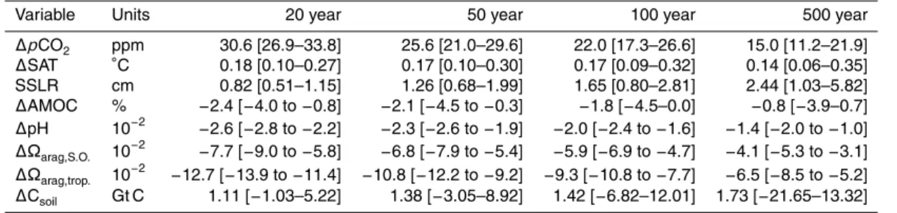
Abstract

Information on the relationship between cumulative fossil carbon emissions and multi-ple climate targets are essential to design emission mitigation and climate adaptation strategies. In this study, the transient responses in different climate variables are quanti-fied for a large set of multi-forcing scenarios extended to year 2300 towards stabilization

5

and in idealized experiments using the Bern3D-LPJ carbon-climate model. The model outcomes are constrained by 26 physical and biogeochemical observational data sets in a Bayesian, Monte-Carlo type framework. Cumulative fossil emissions of 1000 Gt C result in a global mean surface air temperature change of 1.88◦C (68 % confidence interval (c.i.): 1.28 to 2.69◦C), a decrease in surface ocean pH of 0.19 (0.18 to 0.22),

10

and in steric sea level rise of 20 cm (13 to 27 cm until 2300). Linearity between cumu-lative emissions and transient response is high for pH and reasonably high for surface air and sea surface temperatures, but less pronounced for changes in Atlantic Merid-ional Overturning, Southern Ocean and tropical surface water saturation with respect to biogenic structures of calcium carbonate, and carbon stocks in soils. The slopes of

15

the relationships change when CO₂ is stabilized. The Transient Climate Response is constrained, primarily by long-term ocean heat observations, to 1.7◦C (68 % c.i.: 1.3 to 2.2◦C) and the Equilibrium Climate Sensitivity to 2.9◦C (2.0 to 4.2◦C). This is consis-tent with results by CMIP5 models, but inconsisconsis-tent with recent studies that relied on short-term air temperature data affected by natural climate variability.

20

1 Introduction

How multiple climate targets are related to allowable carbon emissions provides basic information to design policies aimed to minimize severe or irreversible damage by an-thropogenic climate change (Steinacher et al., 2013). The emission of carbon dioxide by fossil fuel burning is by far the most dominant driver of the ongoing anthropogenic

25

climate change and of ocean acidification (IPCC, 2013). The increase of a broad set

(3)

BGD

12, 9839–9877, 2015

emissions

Title Page

Tables Figures

◭ ◮

Back Close

Full Screen / Esc

Discussion

P

a

per

|

Discussion

P

a

per

|

Discussion

P

a

per

|

Discussion

P

a

per

|

of climate variables such as atmospheric carbon dioxide (CO₂), CO₂radiative forcing, global air surface temperature or ocean acidification depends on cumulative carbon emissions (Allen et al., 2009; IPCC, 1995). The sum of all carbon emissions, rather than the annual emission flux, is relevant as fossil CO₂accumulates in the climate sys-tem. It is thus informative to quantify the link between cumulative carbon emissions and

5

climate parameters. It is also important to quantify the uncertainty in this link by using probabilistic, observation-constraint approaches or multi-model ensembles. This en-ables one to establish a budget for the amount of allowable carbon emissions if a given target or a set of targets is to be met with a given probability.

The goal of this study is to establish the relation between cumulative carbon

emis-10

sions and changes in illustrative, impact-relevant Earth System parameters such as surface air temperature, sea surface temperature, sea level, ocean acidity, carbon stor-age in soils, or ocean overturning. The linearity between the responses in the different variables and cumulative carbon emissions is investigated. We quantify uncertainties related to specific greenhouse gas emission trajectories, i.e. scenario uncertainty, and

15

those associated with uncertainties in the response to a given emission trajectory by analyzing responses to carbon emission pulses as well as to a set of 55 scenarios rep-resenting the evolution of carbon dioxide and other radiative agents. The response un-certainties are constrained by 26 observational data sets in a Bayesian, Monte-Carlo-type framework with an Earth System Model of Intermediate Complexity. The model

20

features spatially-explicit representation of land use forcing, vegetation and carbon dy-namics, as well as physically consistent surface-to-deep transport of heat and carbon by a 3-D, dynamic model ocean, thereby partly overcoming deficiencies identified for box-type models used in earlier probabilistic assessments (Shindell, 2014a, b). This allows us to reassess the probability density distribution, including best estimates and

25

(4)

BGD

12, 9839–9877, 2015

emissions

Title Page

Tables Figures

◭ ◮

Back Close

Full Screen / Esc

Discussion

P

a

per

|

Discussion

P

a

per

|

Discussion

P

a

per

|

Discussion

P

a

per

|

A climate target that is currently recognized by most world governments (United Na-tions, 2010) places a limit of two degrees Celsius on the global mean warming since preindustrial times. Yet, the United Nations Framework Convention of Climate Change (United Nations, 1992) has multiple objectives. It calls for the avoidance of dangerous anthropogenic interference within the climate system as well as to allow for ecosystems

5

to adapt naturally to climate change, to ensure food production, and to enable sustain-able economic development. These objectives cannot be encapsulated in one single target but may require multiple targets. These may be specific for individual regions and components of the climate system, which includes the atmosphere, hydrosphere, biosphere and geosphere and their interactions (United Nations, 1992). Targets may

10

include bounds for ocean acidification that threatens marine ecosystem functioning and services (IPCC, 2014). Ocean acidification is, like global warming, progressing with anthropogenic CO2 emissions, but, unlike global warming, largely independent of the emissions and atmospheric abundance of non-CO₂forcing agents. In general, the quantitative relationship to emissions and its uncertainty ranges are distinct for different

15

individual target variables.

Climate projections are associated with two fundamentally distinct types of uncer-tainties (e.g. Hawkins and Sutton, 2009). First, the scenario uncertainty arises from the fact that future anthropogenic emissions are not known because they depend largely on human actions and decisions, such as climate policies, technological advances, and

20

other socio-economic factors. Second, the limited understanding of the response of the coupled Earth system to the emissions for a given scenario constitutes an additional uncertainty (model or response uncertainty).

Well defined metrics of the Earth system response to a given forcing are useful to quantify the response uncertainty, and to compare results from different sources, such

25

as ensemble model simulations, model intercomparisons, or observation-based esti-mates. The transient climate response (TCR) and the equilibrium climate sensitivity (ECS) are such metrics, which are used to quantify the global mean surface air tem-perature (SAT) change associated with a doubling of atmospheric CO₂(e.g. Knutti and

(5)

BGD

12, 9839–9877, 2015

emissions

Title Page

Tables Figures

◭ ◮

Back Close

Full Screen / Esc

Discussion

P

a

per

|

Discussion

P

a

per

|

Discussion

P

a

per

|

Discussion

P

a

per

|

Hegerl, 2008). The TCR measures the short-term response (i.e. the temperature in-crease at the time of doubling CO2 in a simulation with 1 % yr

−1

increase), while the ECS quantifies the long-term response after reaching a new equilibrium of the system under the increased radiative forcing. TCR and ECS are metrics for the physical climate system and depend on the rate of ocean heat uptake and multiple feedbacks such as

5

the water vapor, the ice-albedo, or the cloud feedbacks, but they do not depend on the carbon cycle response (Huber and Knutti, 2014; Kummer and Dessler, 2014).

Certain metrics are helpful to reduce the scenario-dependency of results, which may facilitate the communication in a mitigation policy context (Allen and Stocker, 2014). One such metric is the response to a pulse-like emission of CO₂ and other forcing

10

agents as applied to compute global warming potentials in the basket approach of the Kyoto protocol (Joos et al., 2013; Myhre et al., 2013). Another metric is the transient climate response to cumulative carbon emissions (TCRE), which links the global mean temperature increase to the total amount of carbon emissions. In addition to the phys-ical climate response, these metrics also depend on the response of the carbon cycle

15

and thus quantify the response uncertainties of both. TCRE is an interesting metric because it has been shown that global warming is largely proportional to cumulative carbon emissions and almost independent of the emission pathway (Allen et al., 2009; Matthews et al., 2009; Zickfeld et al., 2009; IPCC, 2013; Gillett et al., 2013). It essen-tially represents the combination of the TCR and the cumulative airborne fraction of

20

CO2(Collins et al., 2013).

There is an apparent discrepancy between the TCR estimated with the most recent set of Earth System Models (ESM) vs. some recent studies, suggesting the possi-bility of a low TCR (Collins et al., 2013). Shindell (2014a, b) suggest that there are biases in simple models that do not adequately account for the spatial distribution of

25

(6)

proba-BGD

12, 9839–9877, 2015

emissions

Title Page

Tables Figures

◭ ◮

Back Close

Full Screen / Esc

Discussion

P

a

per

|

Discussion

P

a

per

|

Discussion

P

a

per

|

Discussion

P

a

per

|

bilistic twenty-first century projections based on simple models and observational con-straints under-weight the possibility of high impacts and over-weight low impacts on multi-decadal timescales. Huber and Knutti (2014) find that the TCR and ECS of the ESMs are consistent with recent climate observations when natural variability and up-dated forcing data are considered. Kummer and Dessler (2014) concluded that

consid-5

ering a≈33 % higher efficacy of aerosol and ozone forcing than for CO2forcing would resolve the disagreement between estimates of ECS based on the twentieth century observational record and those based on climate models, the paleoclimate record, and interannual variations. Yet, an updated probabilistic quantification of the TCR, ECS, and TCRE with a spatially-explicit model and constrained by a broad set of observations is

10

missing.

2 Methods

2.1 Modeling framework

We apply the Bern3D-LPJ model in a Bayesian approach which is described in detail by Steinacher et al. (2013). The Bern3D-LPJ is an Earth system Model of Intermediate

15

Complexity (EMIC) that consists of a three-dimensional dynamic ocean component (Müller et al., 2006; Parekh et al., 2008) including sea-ice (Ritz et al., 2011a), a two-dimensional energy and moisture balance model of the atmosphere (Ritz et al., 2011a, b), and a comprehensive terrestrial biosphere model with dynamic vegetation (Sitch et al., 2003), permafrost, peatland (Spahni et al., 2012), and land-use (Strassmann

20

et al., 2008) modules.

We rely here on simulations presented by Steinacher et al. (2013) as briefly de-scribed in the following and illustrated in Fig. 1. Uncertainties in physical and carbon-cycle model parameters, radiative efficiencies, climate sensitivity, and carbon-cycle feedbacks are taken into account by varying 19 key model parameters to

gener-25

ate a model ensemble with 5000 members (Table S1 in Steinacher et al., 2013). 26

(7)

BGD

12, 9839–9877, 2015

emissions

Title Page

Tables Figures

◭ ◮

Back Close

Full Screen / Esc

Discussion

P

a

per

|

Discussion

P

a

per

|

Discussion

P

a

per

|

Discussion

P

a

per

|

observation-based data sets are used to constrain the model ensemble by assigning skill scores to each ensemble member. The observational data sets combine informa-tion from satellite, ship-based, ice-core, and in-situ measurements to probe both the mean state and transient responses in space and time. The data sets are organized in a hierarchical structure (Fig. S3 and Table S2 in Steinacher et al., 2013) with the four

5

main groups “CO2” (atmospheric record and ocean/land uptake rates), “Heat” (surface air temperature and ocean heat uptake), “Ocean” (3-D fields of seven physical and biogeochemical tracers), and “Land” (seasonal atmospheric CO2change, land carbon stocks, fluxes, and fraction of absorbed radiation). From the simulation results over the historical period (“mod”) and the set of observational constraints (“obs”), we assign

10

a score to each ensemble membermasS_m∝exp(−₂1(Xmmod−Xobs)2

σ2 ). This likelihood-type

function basically corresponds to a Gaussian distribution of the data-model discrep-ancy (Xmmod−Xobs) with zero mean and varianceσ2, which represents the combined model and observational error. The overbar indicates that the error-weighted data-model discrepancy is first averaged over all data points of each observational variable

15

(volume or area-weighted) and then aggregated in the hierarchical structure by aver-aging variables belonging to the same group. 3931 out of the 5000 ensemble members contribute less than a percent to the cumulative skill of all members and are not used any further.

In a next step we run the constrained model ensemble for 55 greenhouse gas

sce-20

narios spanning from high business-as-usual to low mitigation pathways. The set of scenarios consists of economically feasible multi-gas emission scenarios from the in-tegrated assessment modeling community. In addition to the four RCP scenarios (Moss et al., 2010) that were selected for the fifth assessment report of the IPCC, we included 51 scenarios from the EMF-21 (Weyant et al., 2006), GGI (Grübler et al., 2007), and

25

(8)

BGD

12, 9839–9877, 2015

emissions

Title Page

Tables Figures

◭ ◮

Back Close

Full Screen / Esc

Discussion

P

a

per

|

Discussion

P

a

per

|

Discussion

P

a

per

|

Discussion

P

a

per

|

the conservative assumption of constant aerosol emissions at the level of the year 2005, which implies a significant cooling effect continued into the future in these sce-narios. The scenarios are extended from 2100 to 2300 by stabilizing atmospheric CO2 and the non-CO₂forcing by the year 2150 (see Steinacher et al., 2013, for details).

In addition to these multi-gas scenarios used by Steinacher et al. (2013), we run the

5

model ensemble for an idealized “2xCO2” scenario to determine TCR and ECS and

an emission pulse experiment. In the 2xCO₂simulation, atmospheric CO₂is increased by 1 % yr−1 from preindustrial levels until a doubling of the concentration is reached. After that, the CO2 concentration is held fixed. All other forcings remain constant at preindustrial levels. The emission pulse simulations are conducted as described by

10

Joos et al. (2013). A pulse input of 100 Gt C is added to a constant background CO₂ concentration of 389 ppm in year 2010, while all other forcings are held constant at 2010 levels. The impulse response function (IRF) is then derived from the difference between simulations with and without emission pulse. Additionally, experiments with pulse sizes of 1000, 3000, and 5000 Gt C were performed to test the sensitivity of the

15

response to the pulse size. These additional pulse experiments were run for a model configuration with median parameter settings, able to reproduce the median response of the ensemble for the 100 Gt C pulse (Fig. 2).

2.2 Different definitions of TCRE and calculation of probability density

functions

20

There are slightly different definition of TCRE. Matthews et al. (2009) defines it similar to the TCR, i.e. as the ratio of warming to cumulative CO2 emissions in a simulation with prescribed 1 % yr−1 increase in CO2 at the time when CO2 reaches double its preindustrial concentration. In the Fifth Assessment Report (AR5) of the IPCC, on the other hand, TCRE is defined more generally as the annual mean global surface

tem-25

perature change per unit of cumulated CO2 emissions in a scenario with continuing emissions (Collins et al., 2013). In scenarios with non-CO2forcings, such as the

(9)

BGD

12, 9839–9877, 2015

emissions

Title Page

Tables Figures

◭ ◮

Back Close

Full Screen / Esc

Discussion

P

a

per

|

Discussion

P

a

per

|

Discussion

P

a

per

|

Discussion

P

a

per

|

sentative concentration pathways (RCPs), the diagnosed TCRE thus also depends on the non-CO2 forcing. Further, the transient response should be distinguished from the peak response to cumulative emissions as defined in Allen et al. (2009), although the TCRE is nearly identical to the peak climate response to cumulative carbon emissions in many cases (Collins et al., 2013).

5

In this study, the transient and peak responses per cumulative emissions at a given timetare defined as

TCRE(t)=X(t)

E(t) (1)

TCREpeak(t)=

maxt′_≤_t(X(t′))

E(t) , (2)

whereX(t) is one of the target variables (e.g. global mean surface temperature change)

10

andE(t) are the cumulative CO2 emissions (either total or fossil-fuel only emissions; see Sect. 2.4). For the transient response analyses, TCRE(t) is taken into account for every year 2000< t≤2300 (i.e. 300 data points per simulation), whereas the peak response is evaluated only once at the end of a simulation, i.e. TCRE_peak(t=2300).

Cumulative carbon emissions E_m,s(t) and climate response Xm,s(t) are diagnosed

15

for each model configuration 1≤m≤N_m (N_m=1069), greenhouse-gas scenario 1≤

s≤Ns (Ns=55), and simulation year 2000< t≤2300. For each model configuration

m, the plausible range ofX for a givenE is then derived from the convex hull of the points (E_m,s(t),Xm,s(t)) for the different scenarioss(and different yearstin the case of the transient response). By adding the convex hulls from all model configurationsmin

20

(10)

BGD

12, 9839–9877, 2015

emissions

Title Page

Tables Figures

◭ ◮

Back Close

Full Screen / Esc

Discussion

P

a

per

|

Discussion

P

a

per

|

Discussion

P

a

per

|

Discussion

P

a

per

|

for eachE, the relative probability mapprel(E,X) is calculated:

prel(E,X)=

p(E,X) max

X (p(E,X))

(3)

p(x,y)=X

m

θm(x,y)Sm (4)

θm(x,y)=

(

1, if (x,y)∈C({(Em,s,Xm,s), s=1,. . .,Ns})

0, otherwise, (5)

where C(P) denotes the convex hull of the set of points P. For given emissions E,

5

prel(E,X) represents the probability density function of the response in X to these emissions.

2.3 Testing the linearity of the response

From the probability maps in the (E,X) space probability density functions are extracted atE=1000, 2000, and 3000 Gt C. To compare the response at different emission

lev-10

els the PDFs at 2000 and 3000 Gt C are rescaled to the response per 1000 Gt C. In a perfectly linear system we would expect that the rescaled PDFs are identical for the different emission levels. To test the linearity of the response further, we fit a linear func-tion ˆX(E)=aX·E to the points (Em,s(t),Xm,s(t)) for each model configurationm. The linear function is forced through zero because we requireX(E =0)=0 at preindustrial

15

(t=1800). From the obtained coefficients a_X_,_m of the model ensemble, we then cal-culate a PDF for the sensitivityaX of the response to cumulative emissions under the assumption that a linear fit is reasonable. The goodness of fit is quantified by the

corre-lation coefficients,r_m, and standard errors of the regression,σ_m=

r

P

s(Xm,s−Xˆ(Em,s))2

Ns , for

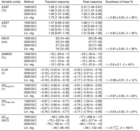
each model setupm. In Table 2, the ensemble median and 68 %-range ofr_m, as well

20

as the ensemble median standard error (expressed as as percentage of the median linear slope), ˆσ, are reported.

(11)

BGD

12, 9839–9877, 2015

emissions

Title Page

Tables Figures

◭ ◮

Back Close

Full Screen / Esc

Discussion

P

a

per

|

Discussion

P

a

per

|

Discussion

P

a

per

|

Discussion

P

a

per

|

2.4 Total vs. fossil-fuel only carbon emissions

Many studies report TCRE with respect to “cumulative total anthropogenic CO2 emis-sions” (e.g. IPCC, 2013; Allen et al., 2009; Meinshausen et al., 2009), not distinguish-ing between fossil-fuel emissions and emissions from land-use changes. Here, we use a model that explicitly simulates terrestrial carbon fluxes, including those from land-use

5

changes. Thus the diagnosed carbon emissions obtained by closing the global carbon budget to match the prescribed atmospheric concentration in the scenarios correspond to fossil-fuel emissions only. In order to estimate total emissions in our simulations, di-rect land-use emissions (i.e. carbon from vegetation that is removed due to land-use changes) are instantaneously added to the diagnosed fossil-fuel emissions. The

de-10

layed emission of carbon from deforestation via product and litter pools as well as indirect land-use change effects such as the losses of terrestrial sink capacity (Strass-mann et al., 2008) or from the abandonment of land-use areas are simulated by the model, but they are not included in the estimate of total carbon emissions because this would require additional simulations. Shifting cultivation (Stocker et al., 2014) has

15

not been considered in this study. Results in the present study are mostly given as a function of total (fossil-fuel plus deforestation) and, where indicated, additionally as a function of fossil-fuel emissions.

3 Results

3.1 Climate response to an emission pulse

20

In a first step, we explore how different climatic variables respond to a pulse-like input of carbon into the atmosphere (Fig. 2). Impulse Response Functions (IRF) for CO2, SAT, steric sea level rise (SSLR), and ocean and land carbon uptake are given elsewhere and we refer the reader to the literature for a general discussion on IRFs, underlying carbon cycle and climate processes, and time scales (e.g. Archer et al., 1998; Joos

(12)

BGD

12, 9839–9877, 2015

emissions

Title Page

Tables Figures

◭ ◮

Back Close

Full Screen / Esc

Discussion

P

a

per

|

Discussion

P

a

per

|

Discussion

P

a

per

|

Discussion

P

a

per

|

et al., 2013; Maier-Reimer and Hasselmann, 1987; Shine et al., 2005). CO₂ is added instantaneously to the model atmosphere to determine IRFs. This results in a sudden increase in CO2and radiative forcing. Afterwards, the evolution in the perturbation of atmospheric CO₂ and in any climate variable of interest, e.g. global mean surface air temperature, is monitored in the model. The resulting curve is the impulse response

5

function (Fig. 2). Here, 1069 runs were carried out in different model configurations

by adding emissions of 100 Gt C to an atmospheric CO₂ background concentration

of 389 ppm, which corresponds to the concentration in the year 2010. Additionally, simulations with emission pulses of 1000, 3000 and 5000 Gt C were run for a median model configuration (Methods). For comparability, all IRFs are normalized to a carbon

10

input of 100 Gt C.

The motivation is two-fold. First, the dynamic of a linear (or approximately linear sys-tem) is fully characterized by its response to a pulse-like perturbation, i.e., the response of variableX at yeartto earlier annual emissions,e, at yeart′can be represented as the weighted sum of all earlier annual emissions. The weights are the values of the IRF

15

curve at emission aget−t′:

X(t)=X

t′

e(t′)·IRF(t−t′), (6)

where the sum runs over all years t′ with annual emissions up to year t. IRFs thus provide a convenient and comprehensive quantitative characterization of the response of a model. IRFs form also the basis for the metrics used to compare different

green-20

house gases in the Kyoto basket approach and to compute CO2equivalent concentra-tions (Joos et al., 2013; Myhre et al., 2013) and are used to build substitute models of comprehensive models (Joos et al., 1996). Second and relevant for the TCRE and for this study, IRFs allow us to gage whether there is a roughly linear relationship between cumulative carbon emissions

25

E(t)=X

t′

e(t′) (7)

(13)

BGD

12, 9839–9877, 2015

emissions

Title Page

Tables Figures

◭ ◮

Back Close

Full Screen / Esc

Discussion

P

a

per

|

Discussion

P

a

per

|

Discussion

P

a

per

|

Discussion

P

a

per

|

and the change in a climate variable of interest,X(t). The transient climate response for variableX to cumulative carbon emissions is in this notation:

TCRE(t,X)=X(t)

E(t) (8)

We note that there is a close relationship between Eqs. (6) to (8) and thus between cumulative carbon emissions E(t), response X(t) and TCRE. The IRF provides the

5

link between these quantities.

Three conditions are to be met for a strict linear relationship between cumulative carbon emissionsE and responseX for any emission pathway: (i) the response is in-dependent of the magnitude of the emissions, and (ii) the response is inin-dependent of the age of the emission, i.e., the time passed since emissions occurred. In this case the

10

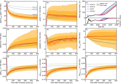
IRF and the TCRE is a constant and all emissions are weighted equally in Eq. (6), (iii) non-CO₂ forcing factors play no role; a point that will be discussed later. While these conditions are not fully met for climate variables, they may still approximately hold for plausible emission pathways. For the range of RCP scenarios, the mean age of the car-bon emissions varies between a few decades to hundred years for the industrial period

15

and up to year 2100, then it increases up to 300 years until 2300 AD (Fig. 2c). More than half of the cumulative carbon emissions have typically an age older than 30 years (Fig. 2c). If the IRF curve is approximately flat after a few decades and independent of the pulse size, then the vast majority of emission is weighted by a similar value in Eq. (6). Consequently, the relationship between responseX(t) and cumulative

emis-20

sions,E(t) is approximately linear and path-independent. This response sensitivity per unit emission,X(t)/E(t), corresponds to an “effective” (emission-weighted) mean value of the IRF and is the TCRE. Indeed, the IRF for many variables varies within a limited range after a few decades (Fig. 2). Then, an approximately linear relationship between

E(t) andX(t) holds and TCRE is approximately scenario-independent.

25

(14)

BGD

12, 9839–9877, 2015

emissions

Title Page

Tables Figures

◭ ◮

Back Close

Full Screen / Esc

Discussion

P

a

per

|

Discussion

P

a

per

|

Discussion

P

a

per

|

Discussion

P

a

per

|

from 30 year to the end of the simulation (500 year) and for the different pulse sizes of 100 to 3000 Gt C. Consequently, we expect a close-to-linear relationship between these variables and cumulative carbon emissions.

For a given pulse size, the median of the IRF for the saturation with respect to arag-onite in the tropical (Ωarag, trop.) and Southern Ocean (Ωarag,S.O.) surface waters and for

5

the global soil carbon inventory varies within a limited range. However, the normalized IRFs for these variables vary substantially with the magnitude of the emission pulse. Thus, we expect a non-linear relationship between the ensemble median responses and cumulative carbon emissions for these quantities.

The atmospheric CO₂perturbation declines by about a factor of two within the first

10

100 years for an emission pulse of 100 Gt C. This means that the CO₂ concentration at a specific time depends strongly on the emission path of the previous 100 years. In addition, the IRF differ for different pulse sizes because the efficiency of the oceanic and terrestrial carbon sinks decreases with higher CO₂ concentrations and warming. The fraction remaining airborne after 500 years is about 75 % for a pulse input of 3000 Gt C,

15

about 2.5 times larger than the fraction remaining for a pulse of 100 Gt C (Fig. 2a). Thus, we do not expect a scenario-independent, linear relationship between atmospheric CO2and cumulative emissions.

The Monte-Carlo IRF experiments allow us also to assess the response or model un-certainty (Fig. 2, orange range). The 90 % confidence range in the IRF are substantially

20

larger than the variation of the (normalized) median IRF for the variables SAT, SSLR, AMOC, and soil carbon inventory. Consequently, the model uncertainty will dominate the uncertainty in TCRE and is larger than uncertainties arising from dependencies on the carbon emission pathway. On the other hand, the response uncertainty from our 5000 Monte Carlo model setups are more comparable to the variation in the median

25

IRFs for atmospheric CO₂, and surface water saturation with respect to aragonite in the tropical ocean and Southern Ocean.

In summary, we expect close-to-linear relationship between cumulative carbon emis-sions and SAT, surface ocean pH, SSLR and AMOC, and less well expressed linear

(15)

BGD

12, 9839–9877, 2015

emissions

Title Page

Tables Figures

◭ ◮

Back Close

Full Screen / Esc

Discussion

P

a

per

|

Discussion

P

a

per

|

Discussion

P

a

per

|

Discussion

P

a

per

|

behavior for global soil carbon and surface water saturation with respect to aragonite. Uncertainty in the response dominate the uncertainty arising from path dependency for SAT, SSLR, AMOC, and soil carbon. In addition to the path dependency and the re-sponse uncertainty in TCRE discussed above, forcing from non-CO₂agents will affect the TCRE. We expect a notable influence of non-CO2 agents on the physical climate

5

variables SAT, SSLR, and AMOC. For example, Strassmann et al. (2009) attributed simulated surface warming to individual forcing components for a range of mitigation and non-mitigation scenarios. They find that non-CO2 greenhouse gas forcing causes up to 50 % as much warming as CO2forcing and that the non-CO2forcing is only partly offset by aerosol cooling by 2100. On the other hand, we expect a small influence of

10

non-CO₂forcing on pH and saturation state which is predominantly driven by the CO₂ perturbation (Steinacher et al., 2009; McNeil and Matear, 2007).

3.2 Climate response to cumulative carbon emissions

In the next step, we investigate the response in multiple climate variables, X(t), as

a function of cumulative carbon emissions E(t). We ran the model ensemble for

15

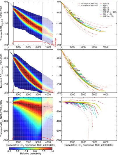
55 multi-gas emission scenarios from the integrated assessment modeling commu-nity which range from very optimistic mitigation to high business-as-usual scenarios (Steinacher et al., 2013, Methods). From those simulations we determine the tran-sient response to cumulative carbon emissions TCRE(t′)=X(t′)/E(t′) (Tables 2 and 3; Figs. 3–6). In addition, we also present results for the peak response TCREpeak(t=

20

2300)=max_t′(X(t′)/E(t=2300)) (Tables 2 and 3, Fig. 3).

We find a largely linear relationship between cumulative carbon emissions and both transient and peak warming (Fig. 3a and b) for the set of emission scenarios consid-ered here. The fact that the results for the transient and peak warming are very similar confirms the finding from the pulse experiment above, i.e. that the response in the

25

global SAT change is largely independent from the pathway of carbon emissions in our model. We note, however, that some low-end scenarios show a non-linear behavior due

(16)

BGD

12, 9839–9877, 2015

emissions

Title Page

Tables Figures

◭ ◮

Back Close

Full Screen / Esc

Discussion

P

a

per

|

Discussion

P

a

per

|

Discussion

P

a

per

|

Discussion

P

a

per

|

due to a strong reduction in the non-CO₂forcing while cumulative emissions continue to increase slightly. Other scenarios (mostly from GGI) deviate from the linear relation-ship when negative emissions decrease the cumulative emissions while the increased temperature is largely sustained. These non-linearities are evident as large changes in the slope between SAT and cumulative emissions towards the end of the individual

5

simulations, that is after≈2150 AD when CO2is stabilized and carbon emissions are low (Fig. 3b). Yet those deviations are not large enough to eliminate the generally linear relationship found for this set of scenarios.

The projected warming for a given amount of carbon emissions is associated with a considerable uncertainty which increases with higher cumulative emissions. This

un-10

certainty arises from both, the response uncertainty of the model ensemble such as the uncertain climate sensitivity or oceanic carbon uptake, as well as from the scenario un-certainty. The scenario uncertainty is mainly due to different assumptions for the non-CO₂ forcing in the scenarios. The AME scenarios, for example, assume a relatively strong negative forcing from aerosols which leads to a consistently smaller warming

15

than in the other scenarios (Fig. 3c). The response and scenario uncertainty appear to be of the same order of magnitude (Fig. 3c).

The transient response is 1.9◦C (Tt C)−1 (1.1–3.4◦C (Tt C)−1 68 % confidence inter-val) evaluated at 1000 Gt C total emissions and similar for 2000 and 3000 Gt C. The median peak warming response is slightly larger. It is 2.3◦C (Tt C)−1(1.5–3.8◦C (Tt C)−1

20

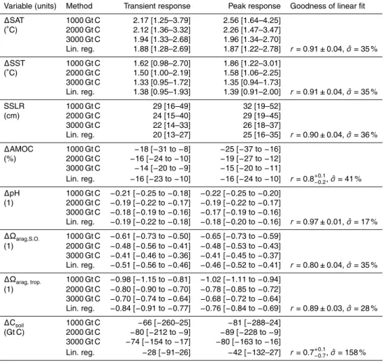
68 % confidence interval) for scenarios with 1000 Gt C total emissions and decreases slightly to 1.9◦C (Tt C)−1(1.3–2.7◦C (Tt C)−1 68 % c.i.) for scenarios with 3000 Gt C to-tal emissions (Fig. 3d). The corresponding responses to fossil-fuel emissions only are accordingly somewhat higher, e.g. 2.2◦C (Tt C)−1(1.3–3.8◦C (Tt C)−1) for the transient response evaluated at 1000 Gt C fossil emissions (Fig. 4, Table 3).

25

We fitted a linear function through zero to the results of each ensemble member and then calculated the probability density functions from the individual slopes. The me-dian slope is 1.8◦C (Tt C)−1(1.1–2.6◦C (Tt C)−1) for the peak response and values are similar for the transient response (Table 2). These slopes are somewhat lower than the

(17)

BGD

12, 9839–9877, 2015

emissions

Title Page

Tables Figures

◭ ◮

Back Close

Full Screen / Esc

Discussion

P

a

per

|

Discussion

P

a

per

|

Discussion

P

a

per

|

Discussion

P

a

per

|

direct results but in general the linear regression approach is able to reproduce the dis-tribution of the peak and transient warming response per 1000 Gt C carbon emissions, although the confidence interval is narrower and the long tail of the distribution might be underestimated.

Following Matthews et al. (2009) and Gillett et al. (2013), we also determined the

5

TCRE for our model ensemble from scenario where atmospheric CO2is increasing by

1 % yr−1until twice the preindustrial concentration is reached. No other forcing agents are included. Correspondingly, we find a slightly lower median TCRE of 1.7◦C (Tt C)−1 (1.3–2.3◦C (Tt C)−1 68 % c.i.; 1.0–2.7◦C (Tt C)−1 5–95 % c.i.) than for the multi-agent scenarios. Gillett et al. (2013) report a TCRE of 0.8–2.4◦C (Tt C)−1(5–95 % range) from

10

15 models of the Coupled Model Intercomparison Project (CMIP5) for a 2xCO2

sce-nario and a range of 0.7–2.0◦C (Tt C)−1estimated from observations. Those ranges are somewhat lower than our 5–95 % ranges of 0.9–3.1◦C (Tt C)−1 obtained by linear re-gression from the scenarios that include non-CO2forcing and 1.0–2.7◦C (Tt C)−1 from the 2xCO2simulations.

15

The transient response in sea surface temperature (SST) shows the same character-istics as the response in SAT. The response is 1.5◦C (Tt C)−1(0.9–2.5◦C (Tt C)−168 % c.i.) evaluated at 1000 Gt C total emissions, and 1.3◦C (Tt C)−1(0.9–1.8◦C (Tt C)−1) for the linear regression approach.

Compared to global mean warming, the responses in steric sea level rise (SSLR)

20

and in the strength of the Atlantic meridional overturning circulation (AMOC) are more emission-path dependent (Fig. 5, right column). In all scenarios applied here, it is as-sumed that atmospheric CO2 and total radiative forcing is stabilized after 2150. This yields a slow additional grow in cumulative emissions after 2150, whereas SSLR con-tinues largely unabated and the AMOC concon-tinues to recover. This results in a steep

25

(18)

BGD

12, 9839–9877, 2015

emissions

Title Page

Tables Figures

◭ ◮

Back Close

Full Screen / Esc

Discussion

P

a

per

|

Discussion

P

a

per

|

Discussion

P

a

per

|

Discussion

P

a

per

|

for the peak SSLR response are somewhat fortuitous and influenced by our choice to stabilize atmospheric CO2and forcings after 2150 in all scenarios.

For AMOC, the peak response is somewhat stronger for low-emission than high-emission paths (Fig. 5c). For 1000 Gt C total high-emissions, we find a peak reduction in AMOC of−24 % (−35 to−16 %) (Fig. 5d). Surface∆pH shows a very tight and linear

5

relationship with cumulative carbon emissions. This is consistent with a small influ-ence of non-CO₂ forcing agents, a small response uncertainty and a relatively small dependency on the carbon emission pathway as revealed by the IRF experiments. For

Ωarag, the non-linearities are more pronounced with a proportionally stronger response at low total emissions (∆Ωarag=−0.68 to−0.54 (Tt C)−1 at 1000 Gt C total emissions)

10

and weaker response at higher total emissions (∆Ωarag=−0.43 to−0.35 (1000 Gt C) −1

at 3000 Gt C total emissions, Fig. 6b and d). Again, results for fossil-fuel emissions only are provided in Fig. 4 and Table 3.

Finally, the change in global soil carbon shows a similar response as SSLR, with continued carbon release from soils after stabilization of greenhouse gas

concentra-15

tions in mid to high emission scenarios. Like the ocean heat uptake, the respiration of soil carbon can be slow, particularly in deep soil layers at high latitudes, and it takes some time to reach a new equilibrium at a higher temperature. The response uncer-tainty represented by the model spread for a given scenario, however, is even larger than the spread from the scenarios. For the same scenario, the 95 % confidence

in-20

terval ranges from a very high loss of up to 40 % to an increases in global soil carbon by a few percent (Fig. 6c). Despite the very broad resulting PDFs, the most likely peak decrease in soil carbon is relatively well represented by the linear regression slope of about−2.3 % (1000 Gt C)−1(Fig. 6b).

In summary, we find that not only global mean surface air temperature, but also the

25

other target variables investigated here show a monotonic relationship with cumula-tive carbon emissions in multi-gas scenarios. The relationship with cumulacumula-tive carbon emission is highly linear for pH as evidenced by the high correlation coefficient and the invariance in the ensemble median and confidence range from total emissions

(19)

BGD

12, 9839–9877, 2015

emissions

Title Page

Tables Figures

◭ ◮

Back Close

Full Screen / Esc

Discussion

P

a

per

|

Discussion

P

a

per

|

Discussion

P

a

per

|

Discussion

P

a

per

|

ble 2). Changes in steric sea level, meridional overturning circulation, and aragonite saturation are generally less linearly related to cumulative emissions than global pH and surface air temperature. These variables show a substantial non-linear response after stabilization of atmospheric CO₂. Nevertheless, the PDF of the peak response for all these variables can be reproduced relatively well with a linear regression yielding

5

correlations ofr=0.8–0.98 and standard errors of ˆσ=30–40 % (Table 2).

3.3 Transient and equilibrium climate sensitivity

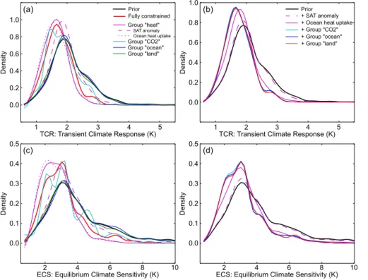
TCR is estimated from the ensemble simulations with 1 % yr−1 increase until doubling of atmospheric CO2 and in combination with the observational constraints (Methods). TCR is constrained to a median value of 1.7 K with 68 and 90 % confidence intervals of

10

1.3–2.2 K and 1.1–2.6 K, respectively. The 68 % range is somewhat narrower than the corresponding IPCC AR5 range of 1.0–2.5 K, (Collins et al., 2013). The CMIP5 model mean and 90 % uncertainty range of 1.8 and 1.2–2.4 K (Flato et al., 2013) are fully consistent with our observation-constraint estimates.

ECS is estimated by extending the 2xCO2simulations by 1500 yr (at constant

radia-15

tive forcing) and fitting a sum of exponentials to the resulting temperature response. Median ECS is 2.9 K with constrained 68 and 90 % confidence interval of 2.0–4.2 K and 1.5–6.0 K. Again, the CMIP5 model mean and 90 % range of 3.2 and 1.9–4.5 K are well within our observation-constrained estimates. However, our 68 % confidence interval is narrower than the IPCC AR5 estimate of 1.5–4.5 K, particularly on the low

20

end.

26 different observational data sets are applied to constrain carbon cycle and physi-cal climate responses. An interesting question is to which extent the different observa-tions can help to reduce uncertainties. Another question is whether some of these data sets may unintentionally deteriorate estimates. Uncertainties in the carbon cycle are

25

(20)

BGD

12, 9839–9877, 2015

emissions

Title Page

Tables Figures

◭ ◮

Back Close

Full Screen / Esc

Discussion

P

a

per

|

Discussion

P

a

per

|

Discussion

P

a

per

|

Discussion

P

a

per

|

The effect of the different observational constraints on the constrained, posterior dis-tribution for TCR and ECS is estimated by applying only subsets of the observational data. This is done in two different ways: first, by giving the subsets of constraints the full weight as if they were the only available data (Fig. 7a and c), and second, by adding subsets of constraints successively with associated weights corresponding to

5

the weights they will have in the fully constrained set (i.e. after adding all the subsets; Fig. 7b and d). As expected, the data groups “land” and “ocean”, targeted towards car-bon cycle responses, do not influence the outcomes for TCR and ECS. The subgroups

“heat” (SAT and ocean heat uptake records) and “CO2” both constrain TCR and ECS

and shift the prior PDF towards the fully constrained PDF when applied alone (Fig. 7a

10

and c). The SAT record tends to constrain TCR and ECS to slightly higher values and the ocean heat uptake data to slightly lower values than the full constraint. When ap-plied sequentially with their corresponding weights in the full constraint, ocean heat uptake represents the strongest constraint, whereas the SAT record changes the prior PDF only slightly (dashed magenta line in Fig. 7b and d). Similarly, adding the group

15

“CO2” after the ocean heat uptake data shifts the PDF only slightly (solid magenta vs. cyan line in Fig. 7b and d). This suggests that the CO₂data does not add substantial information with respect to TCR and ECS that is not already captured by the temper-ature data. In summary, the subgroup “heat” represents the strongest constraints for TCR and ECS. In particular the ocean heat uptake data is important for constraining

20

these metrics.

4 Discussion and conclusions

We have quantified the response of multiple Earth system variables as a function of cu-mulative carbon emissions, the responses to a carbon emission pulse, and two other important climate metrics, the Equilibrium Climate Sensitivity (ECS) and the Transient

25

Climate Response (TCR). Our results are based on (i) a large number of simulations carried out in a probabilistic framework for the industrial period and for the future using

(21)

BGD

12, 9839–9877, 2015

emissions

Title Page

Tables Figures

◭ ◮

Back Close

Full Screen / Esc

Discussion

P

a

per

|

Discussion

P

a

per

|

Discussion

P

a

per

|

Discussion

P

a

per

|

55 different greenhouse gas scenarios and (ii) a diverse and large set of observational data. The observation-constrained probability density functions provide both best esti-mates and uncertainties ranges for risk analyses.

A caveat is that we apply a cost-efficient Earth System Model of Intermediate Com-plexity with limitations in spatial and temporal model resolution and mechanistic

rep-5

resentation of important climate processes. In contrast to box-type or 2-D models applied in earlier probabilistic assessments, the Bern3D-LPX features a dynamic 3-dimensional ocean with physically consistent formulations for the transport of heat, car-bon, and other biogeochemical tracers and includes a state-of-the-art dynamic global vegetation model, peat carbon, and anthropogenic land use dynamics.

10

The focus is on the relationship between cumulative carbon emissions and individual, illustrative climate targets. The probabilistic, quantitative relationship between a climate variable of choice and cumulative carbon emissions permits one to easily assess the ceiling in cumulative carbon emissions if a specific individual limit is not to be exceeded with a given probability. Two examples, cumulative fossil carbon emissions since

prein-15

dustrial must not exceed 640–1030 Gt C (this range indicates the uncertainty from the concurrent non-CO₂ forcing) to meet the Cancun 2◦C target with an 68 % probability by 2100 AD. Cumulative fossil carbon emissions must not exceed 880 Gt C if annual-mean, area-averaged Southern Ocean conditions were not to become undersaturated with respect to aragonite with an 68 % probability (Steinacher et al., 2013).

20

Some aspects are not explicitly considered here. First, meeting a set of multiple targets requires lower cumulative carbon emissions than required to meet the most stringent target within the set in probabilistic assessments (Steinacher et al., 2013). Thus, the evaluation of allowable cumulative emissions to meet multiple climate targets requires their joint evaluation. In practical terms, the joint evaluation of the 2◦C target

25

(22)

BGD

12, 9839–9877, 2015

emissions

Title Page

Tables Figures

◭ ◮

Back Close

Full Screen / Esc

Discussion

P

a

per

|

Discussion

P

a

per

|

Discussion

P

a

per

|

Discussion

P

a

per

|

for the future through existing infrastructure. Consequently, climate target may become out of reach when the transition to a decarbonized economy is delayed (Stocker, 2013). The magnitude of the response is in general non-linearly related to cumulative car-bon emissions. This may present no fundamental problem. Yet, non-linearity in re-sponses add to the scenario uncertainty and extrapolation beyond the considered

sce-5

nario space may not provide reliable results. Non-linear relationships cannot be pre-cisely summarized with one single number. For convenience, we have approximated responses for the investigated variables by linear fits (Tables 2 and 3). A close to linear relationship is found for pH. Consistent with earlier studies, we also find an approxi-mately linear relation between transient surface temperature increase and cumulative

10

carbon emissions of about 1–3◦C (Tt C)−1over our set of multi-agent scenarios. There are some non-linear temperature responses in strong mitigation scenarios (particularly those with negative emissions).

The response to a pulse-like input of carbon into the atmosphere for atmospheric CO2, ocean and land carbon, surface air temperature, and steric sea level rise are

15

discussed elsewhere (e.g. Archer et al., 1998; Frölicher et al., 2014; Joos et al., 2013; Shine et al., 2005). Here we provide in addition impulse response functions for sur-face ocean pH and calcium carbonate saturation states, and soil carbon. A substantial fraction of carbon emitted today will remain airborne for centuries and millennia. The impact of today’s carbon emissions on surface air temperature will accrue within about

20

20 years only, but persists for many centuries. Steric sea level rise accrues slowly on multi-decadal to century time scales. Similar as for CO2, peak impacts in surface ocean pH and saturation states occur almost immediately after emissions and these changes will persist for centuries and millennia. Thus, the environment and the socio-economic system will experience the impact of our current carbon emissions more or less

imme-25

diately and these impacts are irreversible on human time scales.

The recent slow-down in global surface air-temperature warming, termed hiatus, has provoked discussions whether climate models react too sensitive to radiative forcing. Here, the observation-constrained TCR and ECS are quantified to 1.7 and 2.9◦C

(23)

BGD

12, 9839–9877, 2015

emissions

Title Page

Tables Figures

◭ ◮

Back Close

Full Screen / Esc

Discussion

P

a

per

|

Discussion

P

a

per

|

Discussion

P

a

per

|

Discussion

P

a

per

|

semble mean) with 68 % uncertainty ranges of 1.3 to 2.2 and 2.0 to 4.2◦C. Our results for ECS and TCR are consistent with the CMIP5 estimates in terms of multi-model mean and uncertainty ranges (Flato et al., 2013) and there is no apparent discrepan-cies between our observation-constrained TCR and CMIP5 models.

Ocean heat content data provide the strongest constraint on ECS and TCR in our

5

analysis. The influence of the applied long-term hemispheric surface air temperature (SAT) records is smaller. This is not surprising as ocean heat content represents the time-integrated anthropogenic forcing signal both in the observations and in our model. Roemmich et al. (2015) analyzed a large set of ocean temperature measurements from floats covering the top 2000 m of the water column and concluded that ocean

10

heat uptake continues steadily and unabated over the recent period 2006 and 2013. The significant variability in surface temperature and upper 100 m heat content was offset by opposing variability from 100–500 m. The high variability of the SAT and SST records serves to emphasize that they are poor indicator of the steadier subsurface-ocean and climate warming signal. These findings appear to support our approach

15

where ocean heat data provide the strongest constraint on TCR and ECS, comple-mented by hemispheric century-scale (1850 to 2010) SAT records. Studies that rely on decadal-scale SAT (or SST) changes as included in the most recent assessment by the Intergovernmental Panel on Climate Change (IPCC) may be affected by large and unavoidable uncertainties due to the chaotic nature of natural, internal variability.

20

These findings suggest that the downward revision of the ECS range from the IPCC Assessment Report Four to Report Five may, in hindsight, appear perhaps somewhat cautious and that the AR4 range may be more reliable.

Acknowledgements. This study was funded by the Swiss National Science Foundation and the European Project CARBOCHANGE (264879) which received funding from the European 25

(24)

BGD

12, 9839–9877, 2015

emissions

Title Page

Tables Figures

◭ ◮

Back Close

Full Screen / Esc

Discussion

P

a

per

|

Discussion

P

a

per

|

Discussion

P

a

per

|

Discussion

P

a

per

|

References

Allen, M. R. and Stocker, T. F.: Impact of delay in reducing carbon dioxide emissions, Nature Climate Change, 4, 23–26, doi:10.1038/nclimate2077, 2014. 9843

Allen, M. R., Frame, D. J., Huntingford, C., Jones, C. D., Lowe, J. A., Meinshausen, M., and Meinshausen, N.: Warming caused by cumulative carbon emissions towards the trillionth 5

tonne, Nature, 458, 1163–1166, doi:10.1038/nature08019, 2009. 9841, 9843, 9847, 9849 Archer, D., Kheshgi, H., and Maier-Reimer, E.: Dynamics of fossil fuel CO₂neutralization by

ma-rine CaCO₃, Global Biogeochem. Cy., 12, 259–276, doi:10.1029/98GB00744, 1998. 9849, 9860

Calvin, K., Clarke, L., Krey, V., Blanford, G., Jiang, K., Kainuma, M., Kriegler, E., Luderer, G., 10

and Shukla, P. R.: The role of Asia in mitigating climate change: results from the Asia mod-eling exercise, Energ. Econ., 34, S251–S260, doi:10.1016/j.eneco.2012.09.003, 2012. 9845 Collins, M., Knutti, R., Arblaster, J., Dufresne, J.-L., Fichefet, T., Friedlingstein, P., Gao, X. Gutowski, W. J., Johns, T., Krinner, G., Shongwe, M., Tebaldi, C., Weaver, A., and Wehner, M.: Long-term climate change: projections, commitments and irreversibility, chapter 15

12, in: Climate Change 2013: the Physical Science Basis. Contribution of Working Group I to the Fifth Assessment Report of the Intergovernmental Panel on Climate Change, Cambridge University Press, Cambridge, UK, New York, NY, USA, 1029–1136., 2013. 9843, 9846, 9847, 9857

Flato, G., Marotzke, J., Abiodun, B., Braconnot, P., Chou, S. C., Collins, W., Cox, P., Driouech, F., 20

Emori, S., Eyring, V., Forest, C., Gleckler, P., Guilyardi, E., Jakob, C., Kattsov, V., C., R., and Rummukainen, M.: Evaluation of climate models, chapter 9, in: Climate Change 2013: the Physical Science Basis. Contribution of Working Group I to the Fifth Assessment Report of the Intergovernmental Panel on Climate Change, Cambridge University Press, Cambridge, UK and New York, NY, USA, 741–866, 2013. 9857, 9861

25

Frölicher, T. L., Winton, M., and Sarmiento, J. L.: Continued global warming after CO₂emissions stoppage, Nature Climate Change, 4, 40–44, doi:10.1038/nclimate2060, 2014. 9860 Gillett, N. P., Arora, V. K., Matthews, D., and Allen, M. R.: Constraining the ratio of global

warming to cumulative CO₂emissions using CMIP5 simulations, J. Climate, 26, 6844–6858, doi:10.1175/JCLI-D-12-00476.1, 2013. 9843, 9855

30

Grübler, A., Nakicenovic, N., Riahi, K., Wagner, F., Fischer, G., Keppo, I., Obersteiner, M., O’Neill, B., Rao, S., and Tubiello, F.: Integrated assessment of uncertainties in greenhouse

(25)

BGD

12, 9839–9877, 2015

emissions

Title Page

Tables Figures

◭ ◮

Back Close

Full Screen / Esc

Discussion

P

a

per

|

Discussion

P

a

per

|

Discussion

P

a

per

|

Discussion

P

a

per

|

gas emissions and their mitigation: introduction and overview, Technol. Forecast. Soc., 74, 873–886, doi:10.1016/j.techfore.2006.07.009, 2007. 9845

Hawkins, E. and Sutton, R.: The potential to narrow uncertainty in regional climate predictions, B. Am. Meteorol. Soc., 90, 1095–1107, doi:10.1175/2009BAMS2607.1, 2009. 9842

Huber, M. and Knutti, R.: Natural variability, radiative forcing and climate response in the recent 5

hiatus reconciled, Nat. Geosci., 7, 651–656, doi:10.1038/NGEO2228, 2014. 9843, 9844 IPCC: Climate Change 1995: the Science of Climate Change, Technical Summary, Press

Syn-dicate of the University of Cambridge, Cambridge, UK, New York, NY, USA, 1995. 9841 IPCC: Summary for policymakers, in: Climate Change 2013: the Physical Science Basis.

Con-tribution of Working Group I to the Fifth Assessment Report of the Intergovernmental Panel 10

on Climate Change, Cambridge University Press, Cambridge, UK, New York, NY, USA, 3–32, 2013. 9840, 9843, 9849

IPCC: Climate Change 2014: Impacts, Adaptation, and Vulnerability. Contribution of Working Group I to the Fifth Assessment Report of the Intergovernmental Panel on Climate Change, Cambridge University Press, Cambridge, UK, New York, NY, USA, 2014. 9842

15

Joos, F., Bruno, M., Fink, R., Siegenthaler, U., Stocker, T. F., and Le Quéré, C.: An efficient and accurate representation of complex oceanic and biospheric models of anthropogenic carbon uptake, Tellus B, 48, 397–417, doi:10.1034/j.1600-0889.1996.t01-2-00006.x, 1996. 9850 Joos, F., Roth, R., Fuglestvedt, J. S., Peters, G. P., Enting, I. G., von Bloh, W., Brovkin, V.,

Burke, E. J., Eby, M., Edwards, N. R., Friedrich, T., Frölicher, T. L., Halloran, P. R., 20

Holden, P. B., Jones, C., Kleinen, T., Mackenzie, F. T., Matsumoto, K., Meinshausen, M., Plattner, G.-K., Reisinger, A., Segschneider, J., Shaffer, G., Steinacher, M., Strassmann, K., Tanaka, K., Timmermann, A., and Weaver, A. J.: Carbon dioxide and climate impulse re-sponse functions for the computation of greenhouse gas metrics: a multi-model analysis, Atmos. Chem. Phys., 13, 2793–2825, doi:10.5194/acp-13-2793-2013, 2013. 9843, 9846, 25

9849, 9850, 9860

Knutti, R. and Hegerl, G. C.: The equilibrium sensitivity of the Earth’s temperature to radiation changes, Nat. Geosci., 1, 735–743, doi:10.1038/ngeo337, 2008. 9842

Kummer, J. R. and Dessler, A. E.: The impact of forcing efficacy on the equilibrium climate sensitivity, Geophys. Res. Lett., 41, 3565–3568, doi:10.1002/2014GL060046, 2014. 9843, 30

(26)

BGD

12, 9839–9877, 2015

emissions

Title Page

Tables Figures

◭ ◮

Back Close

Full Screen / Esc

Discussion

P

a

per

|

Discussion

P

a

per

|

Discussion

P

a

per

|

Discussion

P

a

per

|

Maier-Reimer, E. and Hasselmann, K.: Transport and storage of CO₂ in the ocean – an inorganic ocean-circulation carbon cycle model, Clim. Dynam., 2, 63–90, doi:10.1007/BF01054491, 1987. 9850

Matthews, H. D., Gillett, N. P., Stott, P. A., and Zickfeld, K.: The proportionality of global warm-ing to cumulative carbon emissions, Nature, 459, 829–832, doi:10.1038/nature08047, 2009. 5

9843, 9846, 9855

McNeil, B. I. and Matear, R. J.: Climate change feedbacks on future oceanic acidification, Tellus B, 59, 191–198, 2007. 9853

Meinshausen, M., Meinshausen, N., Hare, W., Raper, S. C. B., Frieler, K., Knutti, R., Frame, D. J., and Allen, M. R.: Greenhouse-gas emission targets for limiting global warming 10

to 2◦C, Nature, 458, 1158–1162, doi:10.1038/nature08017, 2009. 9849

Moss, R. H., Edmonds, J. A., Hibbard, K. A., Manning, M. R., Rose, S. K., van Vuuren, D. P., Carter, T. R., Emori, S., Kainuma, M., Kram, T., Meehl, G. A., Mitchell, J. F. B., Naki-cenovic, N., Riahi, K., Smith, S. J., Stouffer, R. J., Thomson, A. M., Weyant, J. P., and Wilbanks, T. J.: The next generation of scenarios for climate change research and assess-15

ment, Nature, 463, 747–756, doi:10.1038/nature08823, 2010. 9845

Müller, S. A., Joos, F., Edwards, N. R., and Stocker, T. F.: Water mass distribution and ventilation time scales in a cost-efficient, three-dimensional ocean model, J. Climate, 19, 5479–5499, 2006. 9844

Myhre, G., Shindell, D., Bréon, F.-M., Collins, W., Fuglestvedt, J., Huang, J., Koch, D., Lamar-20

que, J.-F., Lee, D., Mendoza, B., Nakajima, T., Robock, A., Stephens, G., Takemura, T., and Zhang, H.: Anthropogenic and Natural Radiative Forcing, chapter 8, in: Climate Change 2013: the Physical Science Basis. Contribution of Working Group I to the Fifth Assessment Report of the Intergovernmental Panel on Climate Change, Cambridge University Press, Cambridge, UK, New York, NY, USA, 659–740, 2013. 9843, 9850

25

Parekh, P., Joos, F., and Müller, S. A.: A modeling assessment of the interplay between aeolian iron fluxes and iron-binding ligands in controlling carbon dioxide fluctuations during Antarctic warm events, Paleoceanography, 23, PA4202, doi:10.1029/2007PA001531, 2008. 9844 Ritz, S. P., Stocker, T. F., and Joos, F.: A coupled dynamical ocean–energy balance atmosphere

model for paleoclimate studies, J. Climate, 24, 349–375, doi:10.1175/2010JCLI3351.1, 30

2011a. 9844