Development of a system emulating the global carbon cycle in Earth system models

(1)

GMDD

3, 61–97, 2010

System emulating the global carbon cycle

in Earth system models

K. Tachiiri et al.

Title Page

Abstract Introduction

Conclusions References

Tables Figures

◭ ◮

Back Close

Full Screen / Esc

Printer-friendly Version

Interactive Discussion

Geosci. Model Dev. Discuss., 3, 61–97, 2010 www.geosci-model-dev-discuss.net/3/61/2010/ © Author(s) 2010. This work is distributed under the Creative Commons Attribution 3.0 License.

Geoscientific Model Development Discussions

This discussion paper is/has been under review for the journal Geoscientific Model Development (GMD). Please refer to the corresponding final paper in GMD if available.

Development of a system emulating the

global carbon cycle in Earth system

models

K. Tachiiri1, J. C. Hargreaves1, J. D. Annan1, A. Oka2, A. Abe-Ouchi1,2, and

M. Kawamiya1

1

Japan Agency for Marine-Earth Science and Technology 3173-25 Showamachi, Kanazawa-ku, Yokohama, 236-0001, Japan

2

Center for Climate System Research, University of Tokyo, 5-1-5, Kashiwanoha, Kashiwa, Chiba, 277-8568, Japan

Received: 25 December 2009 – Accepted: 12 January 2010 – Published: 3 February 2010

Correspondence to: K. Tachiiri (tachiiri@jamstec.go.jp)

(2)

GMDD

3, 61–97, 2010

K. Tachiiri et al.

Title Page

Tables Figures

◭ ◮

Back Close

Full Screen / Esc

Abstract

By combining the strong points of general circulation models (GCMs), which contain detailed and complex processes, and Earth system models of intermediate complexity (EMICs), which are quick and capable of large ensembles, we have developed a loosely coupled model (LCM) which can represent the outputs of a GCM-based Earth system

5

model using much smaller computational resources.

We address the problem of relatively poor representation of precipitation within our EMIC, which prevents us from directly coupling it to a vegetation model, by coupling it to a precomputed transient simulation using a full GCM. The LCM consists of three com-ponents: an EMIC (MIROC-lite) which consists of a 2-D energy balance atmosphere

10

coupled to a low resolution 3-D GCM ocean including an ocean carbon cycle; a state of the art vegetation model (Sim-CYCLE); and a database of daily temperature, pre-cipitation, and other necessary climatic fields to drive Sim-CYCLE from a precomputed transient simulation from a state of the art AOGCM. The transient warming of the cli-mate system is calculated from MIROC-lite, with the global temperature anomaly used

15

to select the most appropriate annual climatic field from the pre-computed AOGCM

simulation which, in this case, is a 1% pa increasing CO₂concentration scenario.

By adjusting the climate sensitivity of MIROC-lite, the transient warming of the LCM could be adjusted to closely follow the low sensitivity (4.0 K) version of MIROC3.2. By tuning of the physical and biogeochemical parameters it was possible to reasonably

20

reproduce the bulk physical and biogeochemical properties of previously published

CO2stabilisation scenarios for that model. As an example of an application of the LCM,

the behavior of the high sensitivity version of MIROC3.2 (with 6.3 K climate sensitivity) is also demonstrated. Given the highly tunable nature of the model, we believe that the LCM should be a very useful tool for studying uncertainty in global climate change.

(3)

GMDD

3, 61–97, 2010

K. Tachiiri et al.

Title Page

Tables Figures

◭ ◮

Back Close

Full Screen / Esc

1 Introduction

It is now increasingly common for climate models used for projections of climate change to explicitly include representation of the carbon cycle. While atmosphere-only gen-eral circulation models were called AGCMs, and those with coupled oceans termed

AOGCMs, models with more coupled components, which may include various different

5

elements such as ice sheets, atmospheric chemistry and the carbon cycle are increas-ingly called Earth System Models (ESMs), and this is the nomenclature we adopt here. The inclusion of a carbon cycle gives rise to additional sources of uncertainty, on top of those in the physical system, relating to feedbacks in the carbon cycle. The contri-bution of carbon cycle uncertainty to the uncertainty in the transient climate response

10

has been estimated, by Huntingford et al. (2009) using box models to emulate C4MIP ESMs, to be around 40% of that of the uncertainty in equilibrium climate sensitivity and heat capacity. Such uncertainties may have substantial implications for mitigation and adaptation policies relating to climate change. Thus, even as the models increase in complexity and therefore computational cost, it is more important than ever before to

15

be able to perform ensemble integrations in order to investigate uncertainties in the physical and biogeochemical processes, and thus in the climate change projections themselves.

Of course, large ensembles of the most costly models (which are generally designed so as to be capable of running only a handful of simulations on current hardware) are

20

not computationally feasible. Therefore, we inevitably have to simplify the model in some way, and a wide range of so-called Earth System Models of Intermediate Com-plexity (EMICs) have been developed (Claussen et al., 2002). The main distinguishing feature of such models is a reduction in resolution and/or complexity of some model components, resulting in a substantial reduction in computational cost. One common

25

(4)

GMDD

3, 61–97, 2010

K. Tachiiri et al.

Title Page

Tables Figures

◭ ◮

Back Close

Full Screen / Esc

represent the behaviour of more complex GCMs, at least for large-scale physical vari-ables such as globally-averaged surface air temperature on multidecadal to centennial scales (Raper et al., 2001).

A typical limitation of such an EMBM, however, is the inability to represent spatial details of the current climate, such as patterns of precipitation and cloud cover. This

5

is a particular problem when we include sophisticated representations of the carbon cycle, since precipitation and radiation are essential factors for plant life. We wish to ensure that our reduced-complexity model is as traceable as possible to the full GCM, and therefore we would like to use a detailed terrestrial carbon cycle model such as Sim-CYCLE (Ito and Oikawa, 2002) which forms part of the MIROC3.2 ESM

10

(Kawamiya et al., 2005). Thus, we require some way of e_fficiently reproducing the

detailed physical output of GCM in a more efficient EMIC.

Pattern scaling has been proposed as one method for projecting time-varying

cli-mate changes of a GCM in a computationally e_fficient manner (Santer et al., 1990;

Mitchell et al., 1999). In this approach, the spatial pattern of climate change

anoma-15

lies is assumed fixed, and calculated as the difference between a control run (e.g. a

pre-industrial climate simulation) and an equilibrium run under di_fferent boundary

con-ditions, typically 2×CO2with a slab ocean model. For transient simulations, the pattern

of climate change is then scaled by the global mean temperature, which can be calcu-lated using a simpler EMIC, or even derived from an energy balance model. Of course,

20

the validity of this approach depends both on the pattern of climate change being con-stant in time and on it being well represented by the equilibrium integration. While these are reasonable first-order approximations, they introduce a source of error, and therefore additional uncertainty, into the system (Mitchell et al., 1999). Such an ap-proach also generates a deterministic pattern of change which will not include natural

25

variability.

(5)

GMDD

3, 61–97, 2010

K. Tachiiri et al.

Title Page

Tables Figures

◭ ◮

Back Close

Full Screen / Esc

change simulation. The innovation is that rather than using a single climate change pat-tern derived from an equilibrium simulation, we use the transient output from a previous

transient simulation such as the 1% pa 4×CO2runs of the CMIP3 project (Meehl et al.,

2007). For a given global surface temperature anomaly (provided by the EMIC), the year in the transient run that best approximates this temperature anomaly is selected,

5

and the year of climate model data are then used to force the state of the art

terres-trial carbon cycle model. If the trajectory of CO2 mixing ratio of the LCM simulation

matches that of the transient simulation of the state of the art model, the EMIC-based results should accurately mimic the full ESM at a small fraction of the computational cost. For reasonable deviations in the trajectory of the mixing ratio (as might arise

10

through changes in model parameters or emissions scenario), the pattern of climate change from the transient run should still be more accurate than that provided by the scaled equilibrium pattern. We illustrate the approach by emulating two versions of the MIROC3.2 ESM. We introduce the models and coupling methodology in Sect. 2. In Sect. 3 we describe the tuning of the LCM to the lower sensitivity version of MIROC3.2.

15

The discussion and conclusions follow in Sects. 4 and 5.

2 Method

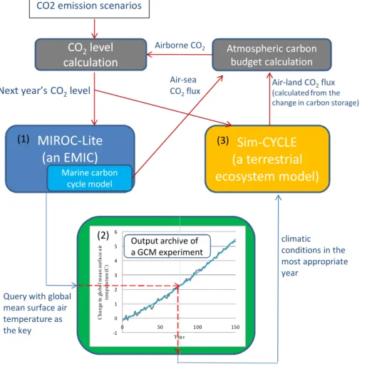
2.1 Basic structure of the loosely coupled model (LCM)

In the LCM system we have developed, three stand-alone models are loosely coupled by unix shell scripting, as opposed to being compiled into a single executable (see

20

Fig. 1). The three models have been described in detail elsewhere, and are now briefly introduced.

2.2 MIROC-lite: an EMIC

MIROC-lite (Oka et al., 2001), the EMIC used in this study, is a simplified version of MIROC3.2 in which the OGCM component is the same (albeit at low resolution) but the

(6)

GMDD

3, 61–97, 2010

K. Tachiiri et al.

Title Page

Tables Figures

◭ ◮

Back Close

Full Screen / Esc

AGCM of MIROC3.2 is replaced by a 2-D energy moisture balance model atmosphere. The model diagnoses the surface air temperature by solving the vertically integrated energy balance equation below.

Ca

∂T

∂t =Qsw−Qlw+Qt−FT (1)

WhereCa is the heat capacity of the air column,T is the surface air temperature, tis

5

time,Qsw andQlw are the net incoming shortwave and outgoing longwave radiation at

the top of atmosphere,Qt is the convergence of the horizontal heat transport by the

atmosphere, andFT is the net downward heat flux at sea/land surface.

The surface wind and the freshwater flux are diagnosed from the distribution of the surface air temperature and the convergence of atmospheric water transport,

respec-10

tively. The meridional wind is decomposed into the Hadley and Ferrel circulations which are considered separately. Both types of circulation are described as proportional to the North-South temperature gradient, and the latitude dependent empirical coef-ficients are determined by a mother GCM (MIROC3.2)’s result. In the current setting, rain and snowmelt on land is returned to the nearest ocean grid.

15

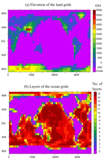
The ocean component of the model is COCO (Hasumi and Suginohara, 1999), an ocean GCM. The version we use in this study includes a sea-ice component. In order to use a long time-step, the acceleration of Bryan (1984) is used in MIROC-lite.

The spatial resolution of the model is 6×6 degree (60×30 grids to cover the entire

globe) and the ocean has 15 layers of unequal thickness (thinner at the surface) down

20

to 5500 m depth. A large diffusivity is given to the first (shallowest) ocean layer, of 50 m

depth, so that it functions as the mixed-layer.

The time step is 36 h and on a single CPU of our SGI Altix 4700, it takes around 15–16 h for 3000 year integration without marine ecosytem. Figure 2 shows the land distribution and the ocean layer.

25

(7)

GMDD

3, 61–97, 2010

K. Tachiiri et al.

Title Page

Tables Figures

◭ ◮

Back Close

Full Screen / Esc

1996) which considers nitrogen, DIC and alkalinity (in addition to the physical ocean’s temperature and salinity), or (2) a carbon cycle model considering marine ecosystem (Palmer and Totterdell, 2001) which includes the above 5 tracers plus phytoplankton, zooplankton and detritus making 8 in total. In this manuscript, (2) is used as it is closer to the ocean carbon cycle used in the MIROC3.2 ESM.

5

We have made some adjustments to the original model. First, we impose a fresh-water flux adjustment to compensate for the poor representation of the freshfresh-water flux from the Atlantic to the Pacific. Following the traditional method for EMICs with 2-D EMBM atmosphere, we set an artificial freshwater flux (FWF) adjustment. Oort (1983)

stated 0.32 Sv in total: with 0.18, 0.17, −0.03 Sv for the bands north of 24 N, 20 S

10

to 24 N, and south of 20 S, respectively. The model’s own internally-generated flux is negligible, and we use Oort’s values for the FWF adjustment.

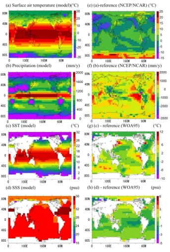
Using the results of FWF adjustment, we obtained acceptable climatology in atmo-spheric temperature, sea surface temperature, sea surface salinity and North Atlantic meridional overturning circulation (see Figs. 3 and 4 for the model after parameter

tun-15

ing), although precipitation (particularly for land) is still not adequate to be coupled with a terrestrial vegetation model.

A second modification is to modify the outgoing longwave parameterisation in order

to both account for forcing through atmospheric CO2concentration (following Table 6.2

of IPCC’s TAR), and also to allow the climate sensitivity (equilibrium temperature

re-20

sponse to 2×CO2) to be varied as by Plattner et al. (2001):

Qlw=A+BT−5.35×ln(pCO2/280)+C·(gT−gTc), (2)

whereA, B are the constants (206.8778 and 1.73357) of the original model; T is the

surface air temperature of the grid concerned;pCO2is the atmospheric CO2

concen-tration (in ppm); gT is the global average SAT; and gT c is gT for 1×CO2. Here we

25

use a standard radiative forcing value (with the coefficient 5.35, the third term results in

3.71 W m−2_{for 2}

×CO2), although the value can change between models. The resultant

(8)

GMDD

3, 61–97, 2010

K. Tachiiri et al.

Title Page

Tables Figures

◭ ◮

Back Close

Full Screen / Esc

2.3 Sim-CYCLE

Sim-CYCLE (Ito and Oikawa, 2002) is a process based terrestrial carbon cycle model, which was developed based on an ecosystem scale model by Oikawa (1985). The origin of these models is in the dry-matter production theory proposed by Monsi and Saeki (1953).

5

In this model, ecosystem carbon storage is divided into plant biomass and soil or-ganic carbon, and they are subdivided into five compartments: foliage, stem, root for plant biomass, and litter and mineral soil for soil organic matter. The model also has a water and radiation process, as carbon dynamics is closely coupled with these pro-cesses. The single-leaf photosynthetic rate (PC) is formulated as a Michaelis-type

10

function of the incident photosynthetic photon flux density (PPFDin):

PC= PCsat·QE·PPFDin

PCsat+QE·PPFDin

, (3)

where PC_sat is PC for the light saturation condition; QE is light-use e_fficiency. PC_sat

and QE are formulated as (maximum value) ×(stress function), where as stresses,

temperature, CO2 level, air humidity and soil water (the parameters are different for

15

C3/C4/crop plants) are taken into consideration.

Ecosystem scale gross primary production (GPP) is calculated under an assumption of exponential attenuation of PAR irradiance due to leaves’ mutual shading.

Autotrophic plant respiration consists of two components: the maintenance respira-tion, and the growth respiration. The amount of the maintenance respiration per unit

20

existing carbon is exponential function of temperature (degree Celsius) with a coeffi

-cient of so called Q10, while the growth respiration is proportional to a net biomass

gain.

ARM∝exp[lnQ10

10 (T−15)] (4)

whereARM andT are the maintenance respiration per unit biomass, and the

temper-25

(9)

GMDD

3, 61–97, 2010

K. Tachiiri et al.

Title Page

Tables Figures

◭ ◮

Back Close

Full Screen / Esc

Soil organic carbon is divided into two conponents: the labile part of litter which circulates once in several months or a year, and the passive part in mineral soil which remains for decades or centuries. Heterotrophic soil respiration is composed of two components for these two. For both, temperature and soil moisture conditions are influential. For temperature dependence, an Arrhenius type function proposed by Lloyd

5

and Taylor (1994) is used.

Sim-CYCLE and the MIROC3.2 AOGCM are two components of an ESM which was

officially used for contributing to IPCC’s AR4.

The distribution of 19 biomes based on the classification of Matthews (1984), the fraction of C4 and crop plants are pre-determined. Thus this is not a dynamic

vegeta-10

tion model. The parameters are determined using observational data of 21 sites for a variety of vegetation types.

Sim-CYCLE has daily time steps and thus needs daily input climatic data (air temper-ature at 2 m hight, precipitation, ground surface tempertemper-ature, soil tempertemper-ature at 10 cm depth, soil temperature at 200 cm depth, specific humidity, wind speed, and ground

15

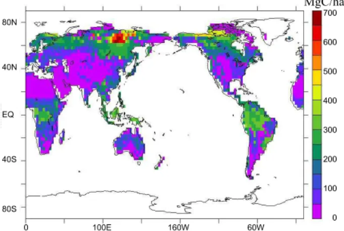
surface radiation). The model can be used in both equilibrium and transient mode. The terrestrial ecosystem total carbon storage after spin-up is presented in Fig. 6.

As Sim-CYCLE has an intermediate complexity, it can readily utilize standard climatic data fields on the typical GCM grid scale and does not need biochemical scale data.

2.4 MIROC3.2: description of the model and the dataset used for the LCM

20

MIROC3.2 is a Japanese coupled GCM, including five physical components: atmo-sphere, land, river, sea ice, and ocean (Hasumi and Emori, 2004). We are using a medium resolution (T42) version of MIROC3.2.

The atmospheric model has 20 vertical σ-layers. The model has an interactive

aerosol module, simplified SPRINTARS (Takemura et al., 2000, 2002), and a land

sur-25

face model MATSIRO (Takata et al., 2003). The ocean component is the same as in MIROC-lite, COCO (Hasumi and Suginohara, 1999). However, the resolution here is

(10)

GMDD

3, 61–97, 2010

K. Tachiiri et al.

Title Page

Tables Figures

◭ ◮

Back Close

Full Screen / Esc

on Oschlies and Garcon (1999) and Oschlies (2001) is used.

MIROC3.2 has two sensitivity versions, one with a sensitivity of 4.0 K (lower

sensi-tivity, LS) and one with a sensitivity of 6.3 K (higher sensisensi-tivity, HS). These only differ in

the cloud treatment, and both of them provide realistic simulations of the mean present climate (Ogura et al., 2008).

5

The difference between the two versions is in the treatment of cloud microphysics.

According to Ogura et al. (2005), there are three differences: (1) mixed phase (i.e.,

solid and liquid) temperature range, (2) form of melted cloud ice, and (3) values of two parameters included in formulations in preciptation rate and sedimentation of cloud

particles. By these differences, the sign of response in cloud condensate to the

dou-10

bled CO₂concentration changed (positive for LS and negative for HS). Yokohata et al.

(2005) compared their response to the Pinatubo volcanic forcing and conclude that LS provided more realistic response, while HS’s response is too strong.

The output of the standard 1% pa compound CO₂ enrichment experiment from

MIROC3.2-LS prepared as part of the CMIP3 experiments for the last IPCC report

15

(AR4) was used as the dataset in this implementation of the LCM. The increment is started from the pre-industrial state. We use one of the three ensemble members. The changes in the annual mean surface air temperature for the 1% incremental run of MIROC3.2-LS/HS are presented as thin light red/blue lines in Fig. 7.

2.5 Coupling method

20

The coupling process (see Fig. 1) is organised as follows.

(0) Spinning up two models (3000 years for MIROC-lite, 2000 years for Sim-CYCLE).

(1) MIROC-lite runs one year with a given CO2 concentration. This may be either

directly prescribed (in the case of a concentration scenario), or in the case of an emis-sions scenario, diagnosed from the previous year’s concentration updated with the

an-25

nual emissions and the feedback from the carbon cycle from previous year (from (3)).

As the marine carbon cycle is also switched on, the amount of CO₂which is absorbed

(11)

GMDD

3, 61–97, 2010

K. Tachiiri et al.

Title Page

Tables Figures

◭ ◮

Back Close

Full Screen / Esc

(2) Using global mean surface air temperature as the key variable, climatic data files of the most suitable year are extracted from the output archive of a preperformed GCM

run with 1% per year CO2 increase for 150 years (described in the previous section).

For the purpose of choosing the year, a quadratic curve is used to smooth the annual mean temperature time series from the GCM data set, and the data set used will

there-5

fore have a mean temperature that differs from the smoothed value due to interannual

variability.

(3) The climatic data set from (2) and the CO₂level determined in (1) are used to drive

Sim-CYCLE for one year. We calculate the change in the total terrestrial ecosystem carbon storage for evaluating the feedback of the terrestrial carbon cycle (note: the

10

albedo and evapotranspiration feedback is not considered here). The total feedback of carbon budget is evaluated by calculating the sum of the terrestrial and marine carbon uptake (obtained in (1)). Then, return to (1).

On our supercomputer (SGI Altix 4700), the system runs one model year in around 1.3 to 1.4 min on a single processor. Thus century-length ensemble integrations are

15

easily achievable.

3 Testing and tuning the LCM

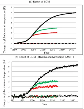
In order to check the performance for a transient run, we reproduced the experiments of Miyama and Kawamiya (2009). These experiments use the state-of-the-art MIROC3.2-LS ESM with oceanic and terrestrial carbon cycle, forced by the stabilisation scenarios

20

of Mueller (2004) (represented as Fig. 8). After fixing the equilibrium sensitivity by

choosing the appropriate value ofCin the previous equation (Eq. 2), we can reproduce

the trend of the MIROC3.-LS’s behaviour in the transient run (thick dark red line in Fig. 7).

Although the default parameter set (with adjusted equilibrium sensitivity as described

25

(12)

GMDD

3, 61–97, 2010

K. Tachiiri et al.

Title Page

Tables Figures

◭ ◮

Back Close

Full Screen / Esc

with perturbed parameters to investigate and tune the response of the model. For the physical parameters, we considered those which have a strong influence on mixing and

circulation in the ocean (i.e., vertical diffusivity, horizontal diffusivity, and GM thickness

diffusion (Gent and McWilliams, 1990)), as these should also influence the ocean’s

carbon uptake.

5

In MIROC-lite, however, there is another very important parameter to determine the

ocean’s carbon uptake. In MIROC-lite, as in MIROC3.2, the air-sea CO2 exchange is

formulated as:

CK×Sl×(pCO2a−pCO2o), (5)

whereCK=a×u2/

q

SC/660 with SC (a function of SST) being the Schmit number,

10

and Sl is solubility (depending on T, S). Unlike MIROC3.2, however, in MIROC-lite

the wind speeduin this equation is fixed as a globally and temporarily constant value,

and this parameter has a large influence in determining the amount of carbon uptake

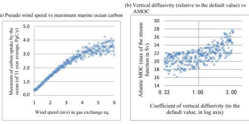
by the ocean. Thus, as depicted in Fig. 9a, this “pseudo” wind speed has large effect

on the ocean’s carbon uptake, while vertical di_ffusivity has some e_ffect on the Atlantic

15

meridional overturning circulation (Fig. 9b).

The output of some of the variables using the best parameter set is presented as Fig. 3a–d. The model has acceptable performance in latitudal change (i.e., the zonal mean is well-reproduced), but the longitudinal change including the land-ocean con-trast is not so well reproduced.

20

When looking at the derivation from the reference (observation or reanalysis) data (Fig. 3e–h), the most obvious problem for the basic MIROC-lite model is, as mentioned in Sect. 1, the precipitation, which does not penetrate into the continental interiors. However, this is not used to drive the Sim-CYCLE terrestrial ecosystem model, and thus has little impact on our simulations. As for the Atlantic meridional overturning, the

25

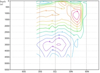
stream function (Fig. 4) is acceptable and the maximum value (20.7 Sv) is close to that of MIROC3.2-LS (20.9 Sv).

(13)

MIROC3.2-GMDD

3, 61–97, 2010

K. Tachiiri et al.

Title Page

Tables Figures

◭ ◮

Back Close

Full Screen / Esc

LS’s behaviour for stabilisation scenarios of 450, 550 and 1000 ppm. Except for short-term variabilities, the LCM reproduced the basic shapes of the curves as well as the

magnitude of the peak values. The only noticeable difference is observed in marine

carbon uptake for 1000 ppm scenario (Fig. 13), indicating the limitation of a model tuned for 450 ppm scenario.

5

For comparison we also performed a similar experiment to mimic the results from MIROC3.2-HS. For this experiment we can only compare the physical outputs as there are no results from a full Earth System Model based on this physical model. Thus,

we reproduce a 1% pa CO2 enrichment senario. Although, in principle, we could

fur-ther tune the ocean physics and the radiative forcing to fit this version, for purposes of

10

demonstration all we changed is the climate sensitivity parameter. The transient

tem-perature change for the 1% pa CO2enrichment experiment is shown as the thick dark

blue line in Fig. 7). Fixing the equilibrium sensitivity for the HS version is successful in

reproducing the MIROC’s transient response for the first 100 years (note that 2_×CO₂

is reached at the 70th year), but after that the difference comes to be non-negligible.

15

Yokohata et al. (2007) and Yokohata et al. (2008) discussed some reasons why models

of similar equilibrium sensitivity can have di_fferent transient response. Primarily, these

are: (1) differences in ocean heat uptake between transient runs, and (2) the

equi-librium sensitivity estimate (which is typically calculated from an AGCM-slab ocean

model) may di_ffer from the true equilibrium response of the coupled system, due to

20

changes in sea ice and ocean circulation. The difference in transient response

be-tween MIROC-HS and MIROC-lite-HS suggests that tuning of ocean physical param-eters relating to the transient response, as carried out by Huntingford et al. (2009), is also needed when the LCM is used for mimicking other ESMs, and that tuning by using

transient response up to 2×CO2may not be sufficient when a model is used for higher

25

CO₂concentration.

(14)

GMDD

3, 61–97, 2010

K. Tachiiri et al.

Title Page

Tables Figures

◭ ◮

Back Close

Full Screen / Esc

As presented in Figs. 10–13, natural variability shown in GCM’s experiment is not reproduced except for the land carbon uptake which was driven by the GCM’s climatic field. We can attempt to represent natural variability in the physical system, by adding a random number term to the radiative forcing calculation. Natural variability is thought to be results from radiative forcing and interactions between components of the climate

5

system. Pelletier (1997) showed that natural variability has a certain power spectrum and Hoerling et al. (2008) stated that multidecadal variabilities are mainly controlled by external radiative forcing due to GHGs, aerosol, solar and volcanic variations.

On the other hand, however, Wigley and Raper (1990) demonstrated that because of the ocean’s large heat capacity, a random white noise forcing results in a red spectrum

10

in the global mean temperature.

With these facts in mind, we concluded that as a start it is reasonable to add a

random number term to Eq. (2). Here we tested 3.46×(RN[0,1]-0.5), where RN[0,1] is

a random number (generated for each year and kept constant in a year) with a uniform

distribution between 0 and 1. The coefficeint 3.46 was determined so that the resultant

15

standard deviation of the random term is the value (1 W m−2_{) which Wigley and Raper}

(1990) mentioned as a suitable standard deviation in interannual radiative forcing. As shown in Fig. 15, by adding this term we could reproduce the natural

variabil-ity and a good by-product is an improved land carbon uptake curve by 3.46×RN[0,1]

(Fig. 15c).

20

Further investigation will be needed for this issue.

4 Discussion

The loosely coupled modelling system introduced by this manuscript reproduces the transient carbon cycle calculations of a full state of the art Earth System Model, at a fraction of the computational cost. Therefore, it should be a powerful tool for

in-25

(15)

GMDD

3, 61–97, 2010

K. Tachiiri et al.

Title Page

Tables Figures

◭ ◮

Back Close

Full Screen / Esc

internal parameters of the ocean GCM and carbon cycle (both terrestrial and ocean).

The different spatial patterns of climate change arising from different climate models

from around the world could in principle be utilised by simply swapping in the results from the CMIP3 database. Thus we believe that the loosely coupled system we present

here can conveniently and efficiently account for all major sources of uncertainty in the

5

climate’s response to elevated CO2levels.

The limitation of the database may generate some problems. For example, for the coupled run with 1000 ppm scenario, the global temperature went out of range of the database at year 2382. While it would in principle be possible to extrapolate the database, this has not been implemented. For century length integrations, however,

10

this is unlikely to be a problem for the 4_×CO₂database.

For long-term equilibration experiments, the climate field of the full system would approach that of an equilibrium experiment rather than the transient that we use. How-ever, even in this case, the standard approach of pattern scaling from an equilibrium (slab ocean) run is not an ideal approach either, since this ignores the issue of ocean

15

response. in any case, we expect our approach to be most accurate during a period of steadily increasing temperature, which probably covers most plausible scenarios at least over the next century. Using transient data may be one reason why the LCM overestimates the ocean’s carbon uptake after the peak, and thus to get a good perfor-mance for the total (accumulated) carbon uptake the peak value should be significantly

20

smaller than the target value (about 2.5 Pg C/y). Figure 16 presents the relation be-tween errors in the peak and the total of the ocean’s carbon uptake and shows that the distribution of the ensemble members do not pass though the origin point (0, 0),

but instead pass through (0,−0.2) and (0.2, 0) meaning that the best performer in one

variable is not be the best one in another indicator. To check whether this is due to

25

(16)

GMDD

3, 61–97, 2010

K. Tachiiri et al.

Title Page

Tables Figures

◭ ◮

Back Close

Full Screen / Esc

Currently, the feedback processes from vegetation to the atmosphere apart from change in the total carbon storage (e.g., change in albedo, evapotranspitration and sensible heat flux) are not considered. We should mention that these changes were not included even in the complex and costly MIROC ESM simulation that we emulate here. As well as considering other realistic river maps, this is also future work. However, it

5

is expected that the effect of sum of these feedbacks will not change the results very

greatly.

5 Conclusions

In order to utilize the strengths of both GCMs and EMICs, we developed a loosely coupled model (LCM) system connecting an EMIC, vegetation model and existing GCM

10

output. We expect the result to be a powerful tool for studying the uncertainty in the carbon cycle and its contribution to the future climate change. The LCM reproduced the basic behaviour of the MIROC3.2 ESM for transient runs very accurately over the 21st century, with a modest error over longer term equilibration scenarios. Using this system we intend, by varying model parameters, to investigate uncertainty, particularly

15

in the carbon cycle components of MIROC3.2, and also to extend the approach to other versions of MIROC and other ESMs.

Acknowledgements. This work is supported by Innovative Program of Climate Change Projec-tion for the 21st Century (of the Ministry of EducaProjec-tion, Culture, Sports, Science and Technology (MEXT), Japan).

20

References

Bryan, K.: Accelerating the convergence to equilibrium of ocean-climate models, J. Phys. Oceanogr., 14, 666–673, 1984. 66

(17)

GMDD

3, 61–97, 2010

K. Tachiiri et al.

Title Page

Tables Figures

◭ ◮

Back Close

Full Screen / Esc

G., Lunkeit, F., Mokhov, I. I., Petoukhov, V., Stone, P., and Wang, Z.: Earth system models of intermediate complexity: closing the gap in the spectrum of climate system models, Clim. Dynam., 18, 579–586, 2002. 63

Edwards, N. R. and Marsh, R. J.: Uncertainties due to transportparameter sensitivity in an effi

cient 3-D ocean-climate model., Clim. Dynam., 24, 415–433, doi:10.1007/s00382-004-0508-5

8, 2005. 63

Gent, P. R. and McWilliams, J. C.: Isopycnal mixing in ocean circulation models, J. Phys. Oceanogr., 20, 150–155, 1990. 72

Gregory, J. M. and Forster, P. M.: Transient climate response estimated from

ra-diative forcing and observed temperature change, J. Geophys. Res., 113, 2008, 10

doi:10.1029/2008JD010405, 2008.

Hasumi, H. and Suginohara, N.: Sensitivity of a global ocean general circulation model to tracer advection schemes, J. Phys. Oceanogr., 29, 2730–2740, 1999. 66, 69

Hasumi, H. and Emori, S.: (edited) K-1 Coupled GCM (MIROC) Description, K-1 Technical Report No.1, http://www.ccsr.u-tokyo.ac.jp/kyosei/hasumi/MIROC/tech-repo.pdf, 2004. 69 15

Hoerling, M., Kumar, A., Eischeid, J., and Jha, B.: What is causing the variability in global mean land temperature?, Geophys. Res. Lett., 35, L23712, doi:10.1029/2008GL035984, 2008. 74 Huntingford, C., Lowe, J. A., Booth, B. B. B., Jones, C. D., Harris, G. R., Gohar, L. K., and Meir, P.: Contributions of carbon cycle uncertainty to future climate projection spread, Tellus B, 61, 355–360, doi:10.1111/j.1600–0889.2009.00414.x, 2009. 63, 73

20

Ito, A. and Oikawa, T.: A simulation model of the carbon cycle in land ecosystems (Sim-CYCLE): a description based on dry-matter production theory and plot-scale validation, Ecol. Model., 151, 143–176, 2002. 64, 68

Kawamiya, M., Yoshikawa, C., Kato, T., Sato, H., Sudo, K., Watanabe, S., and Matsuno, T.: De-velopment of an Integrated Earth System Model on the Earth Simulator, J. Earth Simulator, 25

4, 18–30, 2005. 64

Lloyd, J. and Taylor, J. A.: On the temperature dependence of soil respiration, Funct. Ecol., 8, 315–323, 1994. 69

Matthews, E.: Vegetation, land-use and seasonal albedo data sets: Documentation of archived data sets, NASA Technical Memorandum, No. 86107, p. 12, 1984. 69

30

(18)

GMDD

3, 61–97, 2010

K. Tachiiri et al.

Title Page

Tables Figures

◭ ◮

Back Close

Full Screen / Esc

Mitchell, J. F. B., Johns, T. C., Eagles, M., Ingram, W. J., and Davis, R. A.: Towards the con-struction of climate change scenarios, Clim. Change, 41, 547–581, 1999. 64

Miyama, T. and Kawamiya, M.: Estimating allowable carbon emission for CO2 concentration stabilization using a GCM-Based Earth system model, Geophys. Res. Lett., 36, L19709, doi:10.1029/2009GL039678, 2009. 71

5

Monsi, M. and Saeki, T.: Uber den Lichtfaktor in den Pflanzengesellschaften und seine

Bedeu-tung fur die Stoffproduktion, Jpn. J. Bot., 14, 22–52, in German (English version available

as: On the Factor Light in Plant Communities and its Importance for Matter Production, Ann. Bot., Feb 2005, 95, 549–567, 1953. 68

Mueller, S.: Stabilisation Pathways SP450, SP550, SP650, SP750, SP1000, DSP450,

10

DSP550, OSP350, OSP450, available at http://www.climate.unibe.ch/emicAR4/, 2004. 71, 88

Ogura, T., Emori, S., Webb, M. J., Tsushima, Y., Yokohata, T., Abe-Ouchi, A., and Kimoto, M.:

Climate sensitivity of a general circulation model with di_fferent cloud modeling assumptions,

IAMAS, Beijing, 8 August 2005. 70 15

Ogura, T., Emori, S., Webb, M. J., Tsushima, Y., Yokohata, T., Abe-Ouchi, A., and Kimoto, M.: Towards understanding cloud response in atmospheric GCMs: the use of tendency diagnostics, J. Meterol. Soc. Jpn., 86, 69–79, 2008. 70

Oikawa, T.: Simulation of forest carbon dynamics based on a dry-matter production model i. fundamental model structure of a tropical rainforest ecosystem, Botanical Magazine, 98, 20

225–238, 1985. 68

Oka, A., Hasumi, H., and Suginohara, N.: Stabilization of thermohaline circulation by

wind-driven and vertical diffusive salt transport, Clim. Dynam., 18, 71–83, 2001. 65

Oka, A., Tajika, E., Abe-Ouchi, A., and Kubota, K.: Role of ocean in controlling atmospheric CO2 concentration in the course of global glaciations, Clim. Dynam., to be submitted, 2010. 25

66

Oort, A. H.: Global atmospheric circulation statistics, 1958–1973, NOAA Prof Pap14, pp. 180, 1983. 67

Oschlies, A.: Model-derived estimates of new production: New results point towards lower values, Deep-Sea Res. II, 48, 2173–2197, 2001. 70

30

(19)

GMDD

3, 61–97, 2010

K. Tachiiri et al.

Title Page

Tables Figures

◭ ◮

Back Close

Full Screen / Esc

Palmer, J. R. and Totterdell, I. J.: Production and export in a global ocean ecosystem model, Deep-Sea Res. I, 48, 1169–1198, doi:10.1016/S0967-0637(00)00080-7, 2001. 67

Pelletier, J. D.: Analysis and Modeling of the Natural Variability of Climate, J. Climate, 10, 1331–1342, 1997. 74

Plattner, G.-K., Joos, F., Stocker, T. F., and Marchal, O.: Feedback mechanisms and sensitivities 5

of ocean carbon uptake under global warming, Tellus B, 53, 564–592, 2001. 63, 67

Raper, S. C. B., Gregory, J. M., and Osborn, T. J.: Use of an upwelling-diffusion energy balance

climate model to simulate and diagnose A/OGCM results, Clim. Dynam., 17, 601–613, 2001. 64

Santer, B. D., Wigley, T. M. L., Schlesinger, M. E., and Mitchell, J. F. B.: Developing climate sce-10

narios from equilibrium GCM results, Rep. 47 (Max Planck institut fr Meteorologie, Hamburg), 1990. 64

Takata, K., Emori, S., and Watanabe, T.: Development of the minimal advanced treatments of

surface interaction and runoff, Global Planet. Change, 38, 209–222, 2003. 69

Takemura, T., Okamoto, H., Maruyama, Y., Numaguti, A., Higurashi, A., and Nakajima, T.: 15

Global three-dimensional simulation of aerosol optical thickness distribution of various ori-gins, J. Geophys. Res., 105(D14), 17853–17873, 2000. 69

Takemura, T., Nakajima, T., Dubovik, O., Holben, B. N., and Kinne, S.: Single-scattering albedo and radiative forcing of various aerosol species with a global three-dimensional model, J. Climate, 15, 333–352, 2002. 69

20

Weaver, A. J., Eby, M., Wiebe, E. C., Bitz, C. M., Duffy, P. B., Ewen, T. L., Fanning, A. F.,

Holland, M. M., MacFadyen, A., Matthews, H. D., Meissner, K. J., Saenko, O., Schmittner, A., Wang, H., and Yoshimori, M.: The UVic Earth System Climate Model: Model description, climatology and application to past, present and future climates., Atmos.-Ocean, 39, 361– 428, 2001. 63

25

Wigley, T. M. L. and Raper, S. C. B.: Natural variability of the climate system and detection of

the greenhouse effect, Nature, 344, 324–327, 1990. 74

Yamanaka, Y. and Tajika, E.: The role of the vertical fluxes of particulate organic matter and cal-cite in the oceanic carbon cycle: Studies using an ocean biogeochemical general circulation model, Global Biogeochem. Cycles, 10, 361–382, 1996. 66

30

(20)

GMDD

3, 61–97, 2010

K. Tachiiri et al.

Title Page

Tables Figures

◭ ◮

Back Close

Full Screen / Esc

Yokohata, T., Emori, S., Nozawa, T., Ogura, T., Okada, N., Suzuki, T., Tsushima, Y., Kawamiya,

M., Abe-Ouchi, A., Hasumi, H., Sumi, A., and Kimoto, M.: Different transient climate

re-sponses of two versions of an atmosphere-ocean coupled general circulation model, Geo-phys. Res. Lett., 34, L02707, doi:10.1029/2006GL027966, 2007. 73

Yokohata, T., Emori, S., Nozawa, T., Ogura, T., Kawamiya, M., Tsushima, Y., Suzuki, T., Yuki-5

(21)

GMDD

3, 61–97, 2010

K. Tachiiri et al.

Title Page Abstract Introduction Conclusions References Tables Figures ◭ ◮ ◭ ◮ Back Close

Full Screen / Esc

Printer-friendly Version Interactive Discussion -1 0 1 2 3 4 5 6 0 50 C h a n g e in gl o b a l m e a n su rf a ce a ir te m p e ra tu re (C ) Yea r

MIROC-Lite

(an EMIC)

CO2 emission scenarios

Query with global mean surface air temperature as the key

Next year’s CO₂level

Marine carbon cycle model

CO₂level calculation Air CO (1) (2) Output archive a GCM experim

Airborne 100 150 Yea r

Sim-CYCLE

(a terrestrial

ecosystem model)

climatic conditions in the most appropriate year

Atmospheric carbon budget calculation

Air-land CO₂flux

(calculated from the change in carbon storage)

Air-sea CO2flux

(3)

hive of eriment

orne CO₂

(22)

GMDD

3, 61–97, 2010

K. Tachiiri et al.

Title Page

Tables Figures

◭ ◮

Back Close

Full Screen / Esc

(m)

No. of layers (a) Elevation of the land grids

(b) Layers of the ocean grids 80N

40N

EQ

40S

80S

80N

40N

EQ

40S

80S

0 100E 160W 60W

5000

4500

4000

3500

3000

2500

2000

1500

1000

500

0

-500 Ocean

15 14

13

12 11

10

9 8

7

6 5

4

3 2

1 0 5500

(23)

GMDD

3, 61–97, 2010

K. Tachiiri et al.

Full Screen / Esc

(a) Surface air temperature (model)(°C) (e) (a)-reference (NCEP/NCAR) (°C)

(b) Precipitation (model) (mm/y) (f) (b)-reference (NCEP/NCAR) (mm/y)

(c) SST (model) (°C) (g) (c) - reference (WOA95) (°C)

(d) SSS (model) (psu) (h) (d) - reference (WOA95) (psu) 80N

40N

0

40S

80S

0 100E 160W 60W

80N

40N

0

40S

80S

0 100E 160W 60W

80N

40N

0

40S

80S

0 100E 160W 60W

80N

40N

0

40S

80S

0 100E 160W 60W

80N

40N

0

40S

80S

0 100E 160W 60W

80N

40N

0

40S

80S

0 100E 160W 60W

80N

40N

0

40S

80S

0 100E 160W 60W

80N

40N

0

40S

80S

0 100E 160W 60W 30 10 20 0 -10 -20 -35 25 10 20 0 -10 15 5 -5 -15 400 0 800 1200 1600 2000 -3500 0 1000 2000 -2000 -1000 32 6 14 -2 10 2 18 22 26 -2 -10 -6 2 6 12 24 16 20 28 32 38 -1 -5 -3 1 3 6

(24)

GMDD

3, 61–97, 2010

K. Tachiiri et al.

Title Page

Tables Figures

◭ ◮

Back Close

Full Screen / Esc

80N

40N

0

40S

80S

0 100E 160W 60W

80N

40N

0

40S

80S

0 100E 160W 60W

80N

40N

0

40S

80S

0 100E 160W 60W

80N

40N

0

40S

80S

0 100E 160W 60W

80N

40N

0

40S

80S

0 100E 160W 60W

80N

40N

0

40S

80S

0 100E 160W 60W

80N

40N

0

40S

80S

80N

40N

0

40S

80S

0

500

1000

1500

2000

2500 Depth (m)

3000

3500

4000

5000 4500

5500

60S 30S EQ 30N 60N

Fig. 4.Atlantic meridional overturning circulation. After tuning in Sect. 3. An equilibrium state after a 3000 year spin-up is presented.

(25)

GMDD

3, 61–97, 2010

K. Tachiiri et al.

Full Screen / Esc

Printer-friendly Version Interactive Discussion 80N 40N 0 40S 80S

0 100E 160W 60W

80N

40N

0

40S

80S

0 100E 160W 60W

80N

40N

0

40S

80S

0 100E 160W 60W

80N

40N

0

40S

80S

0 100E 160W 60W

80N

40N

0

40S

80S

0 100E 160W 60W

80N

40N

0

40S

80S

0 100E 160W 60W

80N

40N

0

40S

80S

0 100E 160W 60W

80N

40N

0

40S

80S

0 100E 160W 60W

0.0 1.0 2.0 3.0 4.0 5.0 6.0 7.0

-1.5 -1 -0.5 0 0.5 1 1.5

E q u il ib ri u m cl im at e se n si v it y (K )

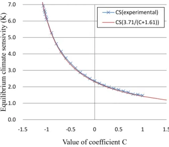
Value of coefficient C

CS(experimental) CS(3.71/(C+1.61))

Fig. 5.Climate sensitivity adjustment. For the red curve, 3.71 (5.35×ln2) is the radiative forcing

(26)

GMDD

3, 61–97, 2010

K. Tachiiri et al.

Title Page

Tables Figures

◭ ◮

Back Close

Full Screen / Esc

MgC/ha

80N

40N

EQ

40S

80S

0 100E 160W 60W

700

600

500

400

300

200

100

0

(27)

GMDD

3, 61–97, 2010

K. Tachiiri et al.

Title Page

Tables Figures

◭ ◮

Back Close

Full Screen / Esc

200 400 600 800 1000 1200 1400 1600 1800 2000

-1 0 1 2 3 4 5 6 7 8

0 50 100 150

C

h

an

g

e

in

g

o

b

al

m

ea

n

su

rf

ac

e

ai

r

te

m

p

er

at

u

re

(K

)

Year

MIROC-LS

MIROC-HS

ML_LS

ML_HS

pCO2

(ppm)

Fig. 7. Change in the annual mean surface air temperature for the 1% incremental run of MIROC3.2-LS/HS and MIROC-lite emulating two versions of MIROC (using the best fit

(28)

GMDD

3, 61–97, 2010

K. Tachiiri et al.

Title Page

Tables Figures

◭ ◮

Back Close

Full Screen / Esc

Interactive Discussion (ppm)

200 300 400 500 600 700 800 900 1000 1100

1850 2050 2250 2450

A

tm

o

sp

h

e

ri

c

C

O

2

c

o

n

c

e

n

tr

a

ti

o

n

(p

p

m

)

Yea r

450ppm

550ppm

1000ppm

(29)

GMDD

3, 61–97, 2010

K. Tachiiri et al.

Full Screen / Esc

Interactive Discussion (b) Vertical diffusivity (relative to the default value) vs

(a) Pseudo wind speed vs maximum marine ocean carbon

5.0

1 2 3 4 5 6

M ax im u m o f ca rb o n u p ta k e b y th e o ce an (o f 3 1 y ea r av er ag e, P g C /y )

Wind speed (m/s) in gas exchange eq.

4.0 3.0 2.0 1.0 0.0 1.00 3.00 0.33

(b) Vertical diffusivity (relative to the default value) vs AMOC 14 16 18 20 22 24 26 28 30 A tl an ti c M O C (m ax o f th e st re am fu n ct io n in S v )

Coefficient of vertical diffusivity (to the default value, in log axis)

1.00 3.00

0.33

(30)

GMDD

3, 61–97, 2010

K. Tachiiri et al.

Title Page

Tables Figures

◭ ◮

Back Close

Full Screen / Esc

Interactive Discussion (a) Result of LCM

-1 0 1 2 3 4 5 6 7

1850 1950 2050 2150 2250 2350 2450

Year

(b) Result of GCM (Miyama and Kawamiya (2009) )

-1 0 1 2 3 4 5 6 7

1850 1950 2050 2150 2250 2350 2450

Change in g

loba

l

m

ea

n

ai

r

te

m

pe

ra

tur

e

(K)

Yea r

Change in g

loba

l

m

ea

n

ai

r

te

m

pe

ra

tur

e

(K)

Fig. 10. Change in air temperature in stabilization experiments. Solid/broken lines are

cou-pled/uncoupled runs, and red/green/black are 450/550/1000 ppm scenarios (in (a)red/green

(31)

GMDD

3, 61–97, 2010

K. Tachiiri et al.

Title Page

Tables Figures

◭ ◮

Back Close

Full Screen / Esc

-1 0 1 2 3 4 5 6 -1 0 1 2 3 4 5 6

1850 1950 2050 2150 2250 2350 2450

Change in

S

T

(

K)

Yea r

Change in

S

T

(

K)

1850 1950 2050 2150 2250 2350 2450

Yea r

Fig. 11.Change in SST in stabilization experiments. Solid/broken lines are coupled/uncoupled

runs, and red/green/black are 450/550/1000 ppm scenarios (in(a)red/green broken lines are

(32)

GMDD

3, 61–97, 2010

K. Tachiiri et al.

Title Page

Tables Figures

◭ ◮

Back Close

Full Screen / Esc

-3 -2 -1 0 1 2 3 4 -3 -2 -1 0 1 2 3 4

1850 1950 2050 2150 2250 2350 2450

A

n

u

a

l c

a

rb

o

n

u

p

ta

k

e

(

P

g

C

/y

)

Yea r

1850 1950 2050 2150 2250 2350 2450

Yea r

A

n

u

a

l c

a

rb

o

n

u

p

ta

k

e

(

P

g

C

/y

)

(33)

GMDD

3, 61–97, 2010

K. Tachiiri et al.

Title Page

Tables Figures

◭ ◮

Back Close

Full Screen / Esc

-1 0 1 2 3 4 5 -1 0 1 2 3 4 5

1850 1950 2050 2150 2250 2350 2450

A

n

u

a

l c

a

rb

o

n

u

p

ta

k

e

(

P

g

C

/y

)

Yea r

A

n

u

a

l c

a

rb

o

n

u

p

ta

k

e

(

P

g

C

/y

)

1850 1950 2050 2150 2250 2350 2450

(34)

GMDD

3, 61–97, 2010

K. Tachiiri et al.

Full Screen / Esc

(a) Surface air temperature

(b) SST -1 0 1 2 3 4 5 6 7 8 9 10

1850 1950 2050 2150 2250 2350 2450

C h a n g e in a ir t e m p e ra tu re ( K) Yea r -1 0 1 2 3 4 5 6 7 8

1850 1950 2050 2150 2250 2350 2450

C h a n g e in S S T ( K) Yea r

(c) Land carbon uptake

(d) Marine carbon uptake

0 1 2 3 4 5

1850 1950 2050 2150 2250 2350 2450

A n n u a l c a rb o n u p ta k e ( P g C /y ) Yea r -3 -2 -1 0 1 2 3 4

1850 1950 2050 2150 2250 2350 2450

A n n u a l c a rb o n u p ta k e (P gC /y ) Yea r

(35)

GMDD

3, 61–97, 2010

K. Tachiiri et al.

Full Screen / Esc

(a) Surface air temperature

(b) SST -1.0 -0.5 0.0 0.5 1.0 1.5 2.0 2.5 3.0

1850 1950 2050 2150 2250

A ir t e m p e ra tu re ( C ) Yea r -0.5 0.0 0.5 1.0 1.5 2.0

1850 1950 2050 2150 2250

S S T (C ) Yea r

(c) Land carbon uptake

(d) Marine carbon uptake -1.5 -1.0 -0.5 0.0 0.5 1.0 1.5 2.0 2.5 3.0

1850 1950 2050 2150 2250

L a n d c a e b o n u p ta k e ( P g C /y ) Yea r -0.5 0.0 0.5 1.0 1.5 2.0 2.5 3.0

1850 1950 2050 2150 2250

M a ri n e c a e b o n u p ta k e ( P g C /y ) Yea r

(36)

GMDD

3, 61–97, 2010

K. Tachiiri et al.

Title Page

Tables Figures

◭ ◮

Back Close

Full Screen / Esc

-1.0 -0.8 -0.6 -0.4 -0.2 0.0 0.2 0.4 0.6 0.8 1.0

-0.8 -0.6 -0.4 -0.2 0.0 0.2 0.4 0.6 0.8 1.0

1

-L

C

M

to

ta

l/

G

C

M

to

ta

l

1-LCMmax/GCMmax

(37)

GMDD

3, 61–97, 2010

K. Tachiiri et al.

Title Page

Tables Figures

◭ ◮

Back Close

Full Screen / Esc

m/sec (a) Wind speed

m/sec (b) Variance of the wind speed Year

Year

5.20

5.10

5.00

4.90

4.80

3.80

3.40 5.00

4.20 4.60