MINIMIZING COMPUTATIONAL ERRORS OF TSUNAMI WAVE-RAY AND TRAVEL TIME
Andrei G. Marchuk
Institute of Computational Mathematics and Mathematical Geophysics, Siberian Division, Russian Academy of Sciences, Novosibirsk, RUSSIA
ABSTRACT
There are many methods for computing tsunami kinematics directly and inversely. The direct detection of waves in the deep ocean makes it possible to establish tsunami source characteristics and origin. Thus, accuracy of computational methods is very important in obtaining reliable results. In a non-homogeneous medium where tsunami wave propagation velocity varies, it is not very easy to determine a wave-ray that connects two given points along a path. The present study proposes modification in the methodology of determining tsunami travel-times and of wave-ray paths. An approximate ray trace path can be developed from a source origin point to any other point on a computational grid by solving directly the problem - and thus obtain the tsunami travel-times. The initial ray approximation can be optimized with the use of an algorithm that calculates all potential variations and applies corrections to travel-time values. Such an algorithm was tested in an area with model bathymetry and compared with a non-optimized method. The latter exceeded the optimized method by one minute of travel-time for every hour of tsunami propagation time.
1. Travel-time computations in non-homogeneous areas.
Numerical modeling of tsunami wave propagation can provide better understanding of the phenomenon. Tsunami wave propagation and travel times can be calculated for different time intervals (isochrones) and various numerical methods have been developed [1]. For areas with complicated geomorphology and bathymetry (islands and narrow straits), travel-time computations based on methods that use Huygen's principle are more effective than others [2]. The basic premise in using this principle requires that all points of the source area where the tsunami wave was generated be sources of omni-directional wave energy radiation. The algorithm for such computation searches through all adjacent grid-points to the generated wave front and calculates the minimum of all tsunami travel time interval through these points.
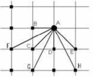
The sum total of all travel-times from the source point to a final point is the minimum for all possible wave travel paths. Rectangular computational grids with known ocean depth values are used normally for travel-times calculations from the source region to all terminal points. Figure 1 shows a grid fragment of such a computational area. The small black squares designate points on the grid, where the wave from the initial tsunami source has arrived and the tsunami travel-times to these grid-points are known.
Fig. 1. The scheme of travel-time determination using Huygens’s principle
We need to find the travel-time from the source up to the point A. Relative to the point A, the neighboring points, where the travel-times are known, there will be the points B, C, D, E, F, G and H. Let the travel-times up to them be equal to T
B, TC, TD, TE, TF, TG and TH respectively.
Between the adjacent grid-points the depth is varying linearly. To determine the tsunami travel-time, we take the distance between two neighboring grid-points L, and a depth value varying from H
1 up to H2. The angle of bottom declination is the auxiliary value
!, which can be designated as
.
Then the tsunami travel-time for that time increment can be expressed as:
(5)
.
Therefore, the tsunami travel-time between the neighboring grid-points is equal to a distance between them divided by the arithmetically averaged velocity of the tsunami at these grid-points. Thus, in order to find the travel-time from the source up to a point A (fig. 1), it is necessary to find a minimum of seven time values
, ,
, , (6)
, ,
,
Where " , " - steps of a grid in horizontal and vertical directions and HA, HB, HC, HE, HF, HG,
HH - the depth values at the corresponding points. Minimum of values Ti (i=1, 2, 3, 4, 5, 6, 7) will
give us the tsunami travel-time from the source up to a point A. In such a way it is possible to find point by point the travel-times to all the points of a computational grid.
As for the neighboring grid-points, the following can be stated. The simplest one is the eight-dot template (Fig. 2).
Fig. 2. The eight-dot template for computation of tsunami travel-times.
In such a template the following eight grid-points: (i-1, j+1), (i, j+1), (i+1, j+1), (i+1, j), (i+1, j-1), (i, j-1), (i-1, j-1), (i-1, j) will be the neighboring ones to point A with the grid coordinates (i, j). The travel-times from each of them to the central point are calculated along eight straight segments. Therefore, this template is sometimes called the eight-radial (eight-dot). However, this template is too simplified and, as a result, the wave front computations from a point source using this template give above the bottom of constant depth an octagonal front line instead of a circle. More precise results can be obtained if for computations use a sixteen-dot (sixteen-radial) template (Figure 3).
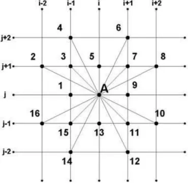
Fig. 3. The sixteen-dot template for tsunami travel-time calculations on a rectangular computational grid.
In this template, the neighbors to the point A, that has the grid coordinates (i, j), are the grid-points
whose indices differ from the grid coordinates of the point A not only by one, but also by some grid-points whose coordinates differ by two (see Figure 3). In this case, if at any of these 16 points the tsunami travel-time is already known, it is possible to find the wave travel-time to point A (at the center of the template).
2. Method for determination of tsunami wave rays in areas with variable depth.
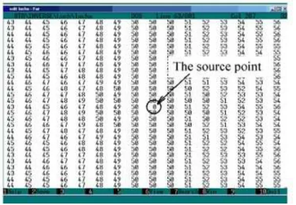
However, the above-described method for travel-time computations does not give directly the traces of the wave rays. In order to determine wave-ray traces with this method, the following algorithm is proposed. Since it is necessary to find the path of the wave ray between two given points in the computational domain, the first step is to calculate travel-times from one of these points to all the other grid points of the computational domain. During the process of travel-time determination at the point (i, j) the grid coordinates of the neighboring point are stored in the computer memory. After completing the computations, two matrices nx (i, j) and ny (i, j) with the dimensions of the whole computational area will be filled. The entries of the first array are the horizontal coordinates and in the second array there are vertical grid coordinates of those points (fig. 4). With the help of these two arrays it is very easy to reconstruct a ray trace from an arbitrary grid-point to the source point. Reconstruction starts at a receiving point.
Fig. 4. Fragment of nx (i, j) array. The source is located at the grid-point (50,50).
Figures 5-6 show an example of the ray reconstruction process in a small sub-section of the entire computational domain. The grid coordinates are indicated at the top and at the left edges of the
Figure. For example, if there is a need to build a wave ray between the points with grid coordinates (10, 10) and (16, 11) (fig.5), the first step will be to calculate travel times in the whole computational domain from the source, which is at point (10, 10). For some of the grid-points in Figure 5 in parentheses we give pairs of numbers from those two arrays nx (i, j) and ny (i, j), which were obtained during travel-time computations.
Fig. 5.
If the reconstruction starts at point (16, 11), the sequence of grid-points, which gives the quickest route for wave propagation from point (10, 10) to point (16, 11) can be easily determined. Conjunction of grid-points (16, 11), (14, 12), (13, 12), (11, 11), (10, 10) gives the tsunami wave ray (see fig, 6). If we draw a line through these points, then we will obtain an approximate ray trace connecting points (10, 10) and (16, 11). The wave rays determined by this method consist of segments of the rays of the template (“star”) (see Figures 2 and 3). When the 8-dot template (see Figure 2) is used, the segments of the defined ray can have only eight variants of direction. When using a 16-dot template, the number of variants increases to 16, which indicates that the approximation to the real wave ray path is significantly improved.
Fig. 6. The reconstruction of the ray trace between two points.
The main disadvantage of these wave-ray determination methods is the limited variety of directions of ray segments. For the 16-dot template this number is 16. Ray traces after this kind of computations are not smooth enough. Figures 7 and 8 show tsunami wave-rays for areas with actual bathymetry. In the Figure 7 the tsunami wave-rays connect the mouth of the Avacha harbor (Southern Kamchatka) and three other points of this area. One point is the Severo-Kurilsk village at the southern part of the area and the other two points are located on the Kamchatka shelf. The next figure (Fig. 8) shows the tsunami wave-ray traces in the eastern part of the Indian Ocean in areas of gradually varying depth (between Nicobar Islands and Sri Lanka) where the wave-rays look like straight lines.
3. Accuracy improvement of the tsunami travel-time computations
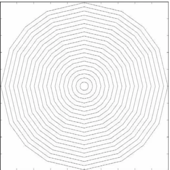
Also, a limited number of ray segment directions cause errors in the determination of the travel-time values at grid-points. These travel-time mismatches can be easily seen in the figure 9, where isolines for travel-time computations at an area with flat bottom are displayed. The dimension of computational area is 1,000x1, 000 points with grid-steps equal to 1 km in both directions and ocean depth being 1,000 m. When the tsunami travel times are determined correctly, the shapes of isochrones must be circles. However, in actuality, instead of circles after the computations we have 16-angle polygons (fig. 9).
Fig. 7. The bottom topography and the wave rays near Kamchatka.
Fig. 8. The bottom topography and the wave rays in the eastern part of the Indian Ocean.
Fig. 9. The test isochrones computation in the area of constant depth using sixteen-dot template (area size 1,000x1, 000, isochrones from 0 to 5,000 seconds with 250 sec steps).
One of the ways to improve the accuracy of approximation is to include more points to the calculation process. For example, it is possible to use a 32-dot template, but in this case the total number of arithmetic operations increases by two times. In addition, the long distances between some points of the template and its center (up to 3 grid-steps) will cause errors in resulting travel-times. The resulting approximation of the wave ray (as shown in the figure 6) consists in a number of straight segments. It is possible to improve significantly the approximation quality by using the technique of variations. Briefly, this means searching for new locations of points along the wave ray. These new points do not have to be grid-points. Within every grid-point included into the calculation the wave ray trace advances with very small incremental steps (1/10 of the grid) in different directions along the grid lines until a new location provides the shorter propagation time along the wave ray path.
To describe the optimization algorithm consideration is given to the small segment of a computational area (figure 10). During the travel-time calculation process, if line SABCD is designated to be the wave-ray trace between the source S and the target point D, the path of the ray
between the source point and any other grid-point can be restored. The procedure for obtaining more precise travel-time values by relocation of points B, C and D is as follows. During the computation process the algorithm will estimate the travel-time at a point B, then the correctional procedure is applied. The grid-point A, which is situated at the ray trace between points S and B, must be relocated along the horizontal and vertical axis within small step (about 1/10 of a grid-step). At every new position of this intermediate point A
1 a travel-time along the trace SA1B will
be calculated, based on the assumption that the depth between two neighboring grid-points varies linearly.
Fig. 10. The scheme of the ray-trace optimization procedure.
The minimum travel-time value will be accepted as the corrected travel-time at point B. It is of great importance that for further computations the corrected travel-time value at point B be used. When the general algorithm (based on the sixteen-dot template) gives the preliminary travel-time value at point C, then the correction procedure must be repeated again for another three grid-points (A, B and C). As a result, a new corrected value of travel-time at a point C will be defined. Such a correctional procedure will be applied to all grid-points along the ray path. Figure 11 shows the result of wave ray optimization with the ray trace indicated above the parabolic bottom slope. In this computational area the depth increases as a squared distance from the left boundary (Y axis). In the left part of the figure the ray is displayed before optimization and in the right part – after optimization. The optimized ray trace is much smoother that the initial one. The shape of optimized ray (right drawing in figure 11) shows a good correlation with the analytical solution, being the segment of a circle. As far as travel-times are concerned, such type of optimization can be applied to the process of travel-times computations. This procedure for a travel-time correction is presented schematically in figure 12.
Fig. 11. The wave ray above the parabolic bottom slope, built using the proposed method. Initial
approximation (left) and optimized by technique of variations (right).
Fig. 12. The scheme of the travel-time correction algorithm.
The segment of a whole 16-dot template is shown in figure 12. The value of travel-time is to be determined at the grid-point A. The minimum travel time value at this point is obtained within a travel-time at the neighboring grid-point C. During previous computations the value of tsunami travel time at point C was determined using the time value at grid-point B. This can be taken from analysis of arrays nx (i, j) and ny (i, j). So, the value at point A was obtained as the sum of travel-time value at point B, plus the wave travel travel-times along segments BC and CA. Then the possibility for the more optimal trajectory of the wave ray must be examined. By relocating point C, it is possible to find a new location of the intermediate point C
1 which can give the minimum travel
time between point B and the grid-point A. Finally this travel-time (along the trace BC
1A) is to be
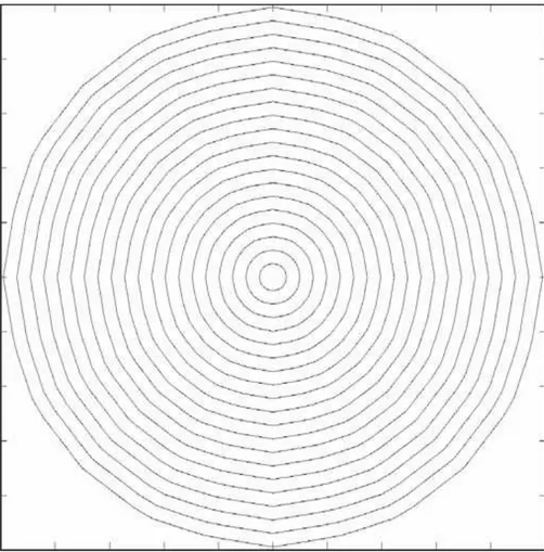
accepted as the corrected travel time at the grid-point A. Using such an optimization procedure the test travel-time computations were carried out for an area of constant water depth. The small round tsunami source is situated in the center of the area defined by 1,000 by 1,000 grid-points. After determination of travel times at all grid-points, tsunami isochrones for every 250 sec of propagation were drawn. The shapes of isochrones by this method are much smoother than for the test without optimization (fig. 9). At some points of the computational area, the travel-time values differ by up to one minute for every one-hour of tsunami wave propagation time. So, for distant tsunamis this error can be significant, which means that the tsunami impact can occurs at least a few minutes earlier than that predicted by traditional methods.
Fig. 13. Test isochrones computation in the area of constant depth using sixteen-dot template with the correction procedure (compare with the Figure 9).
CONCLUSION
A more effective method for solving the wave ray boundary value problem was proposed and tested. The method uses the results of numerical computation of wave travel-times from the source to all other grid points. The method was tested with known exact analytical solutions. Above a flat ocean bottom the time difference between the traditional 16-dot template method and the modified one is estimated to be up to one minute for every one hour of tsunami wave propagation. The proposed method is very effective for wave-ray calculation in 2-D and 3-D non-homogeneous media.
ACKNOWLEDGMENTS
The work was supported by SBRAS Grant for Integration project No. 2006/113, FASI-CRDF contract No. 02.434.11.7016 and RFBR grants 08-05-00300, 08-07-00105.
REFERENCES
1. Marchuk An.G., Chubarov L.B., Shokin Yu.I. Numerical modeling of tsunami waves. Siberian Branch of Nauka Publishers, Novosibirsk, 1983, 175 p. (In Russian).
2. Marchuk An.G. Rules of application of algorithms for tsunami waves kinematic computations that are based on Huygens’ principle. Bulletin of the Novosibirsk Computing Center. Series: Mathematical Problems in Geophysics, Novosibirsk, ICM&MG SD RAS, Issue.5, 1999, p. 93-103.