www.ocean-sci.net/8/65/2012/ doi:10.5194/os-8-65-2012
© Author(s) 2012. CC Attribution 3.0 License.
Ocean Science
Impact of combining GRACE and GOCE gravity data on ocean
circulation estimates
T. Janji´c1, J. Schr¨oter1, R. Savcenko2, W. Bosch2, A. Albertella3, R. Rummel3, and O. Klatt1
1Alfred Wegener Institute for Polar and Marine Research, Bussestrasse 24, 27570, Bremerhaven, Germany 2Deutsches Geod¨atisches Forschungsinstitut, Munich, Germany
3Institute for Astronomical and Physical Geodesy, TU Munich, Munich, Germany
Correspondence to:T. Janji´c ([email protected])
Received: 22 May 2011 – Published in Ocean Sci. Discuss.: 27 June 2011
Revised: 12 January 2012 – Accepted: 23 January 2012 – Published: 8 February 2012
Abstract. With the focus on the Southern Ocean circula-tion, results of assimilation of multi-mission-altimeter data and the GRACE/GOCE gravity data into the finite element ocean model (FEOM) are investigated. We use the geodetic method to obtain the dynamical ocean topography (DOT). This method combines the multi-mission-altimeter sea sur-face height and the GRACE/GOCE gravity field. Using the profile approach, the spectral consistency of both fields is achieved by filtering the sea surface height and the geoid. By combining the GRACE and GOCE data, a considerably shorter filter length can be used, which results in more DOT details. We show that this increase in resolution of measured DOT carries onto the results of data assimilation for the sur-face data. By assimilating only absolute dynamical topogra-phy data using the ensemble Kalman filter, we were able to improve modeled fields. Results are closer to observations which were not used for assimilation and lie outside the area covered by altimetry in the Southern Ocean (e.g. tempera-ture of surface drifters or deep temperatempera-tures in the Weddell Sea area at 800 m depth derived from Argo composite.)
1 Introduction
The vast majority of the observations of the global ocean come from satellite data. Altimetric measurements that mea-sure the sea level height above the reference ellipsoid, are of high accuracy, have near global coverage, are continuous in time, and are available for almost 20 yr. In order to obtain absolute dynamical ocean topography (DOT) that represents the sea level height above the geoid, accurate information about the geoid height is needed. Previously, the geoid height
estimates from the satellite only gravity field models were obtained with the data from the Gravity Recovery and Cli-mate Experiment (GRACE) mission, and before that longer wavelength models were generated from laser and Doppler tracking of geodetic and other satellites. Recently, data from the Gravity field and steady-state Ocean Circulation Explorer (GOCE) satellite became available. Now, GOCE and GRACE satellite data can be combined to obtain a geoid with higher accuracy and spatial resolution (Pail et al., 2010). Although the altimetric sea surface that is needed for compu-tation of DOT still resolves much shorter spatial scales than the geoid computed from the space gravity data, the increase in geoid accuracy and resolution also implies the higher res-olution of DOT. Higher resres-olution spectrally filtered DOT, in addition to other oceanographic information available from in-situ and other space measurements, can be incorporated in general circulation models through data assimilation al-gorithms. This would allow us to predict changes in ocean circulation and to have more accurate estimates of less well observed ocean fields.
ocean model, as an answer to the difference in accuracy be-tween the highly accurate repeat altimetry data and the low accuracy geoid. Later, it became a common practice to sub-tract the average of sea surface height (SSH) from the mea-surements and to replace the average SSH by a separate esti-mate of the mean DOT from the ocean data or unconstrained ocean model. For example, the mean DOT can be obtained by first filtering the difference between the mean sea sur-face – obtained by gridding from along the track the mean altimetric profiles to regular grid – and the geoid. Such an estimate of the mean DOT is combined with drifting buoy velocities (Maximenko et al., 2009) as well as hydrological profiles (Rio et al., 2005, 2009). Also, the mean DOT can be obtained by synthesizing all oceanographic information through inverse modeling (Le Grand et al., 2003). In our study, the mean DOT and its variability are not separated. In-stead, time series of 10 day “absolute” DOTs are generated using the satellite altimetry and our knowledge of the geoid (Skachko et al., 2008) as given by the GOCO1S model. Such a 10 day geodetic DOT time series is then assimilated into the ocean model for one year. The data assimilation method that we will use is ensemble Kalman filtering. The method is de-scribed in detail for assimilation of the geodetic DOT from the altimetry and the GRACE data in Janji´c et al. (2011a,b). Our focus is on the Southern Ocean. We concentrate on the resolution of the DOT and study how different spatial filter-ing impacts ocean circulation estimates.
The first part of the paper will explain the procedure for obtaining the measured DOT as well as the differences in the information content due to the higher data resolution. In the second part of the paper we will examine the impact of the in-creased spectral content of the measured DOT on ocean fields as represented by a finite element ocean model. We will show how we are dealing with the increase in the spectral content of the measured DOT in the data assimilation algorithm. The increase in resolution carries onto the results of data assim-ilation for the surface variables. Finally, we will investigate our results in the Southern Ocean in more detail. By assim-ilating globally the DOT data, the ocean fields in Southern Ocean can be improved even in areas outside the coverage by altimetry. In particular, we will show that by assimilating only the absolute dynamical topography data using the en-semble Kalman filter, we are able to obtain improvements in the Weddell Sea area for temperature at 800 m depth. The Weddell Sea is neither well observed from satellites, nor using conventional observing platforms that are sparse and limited to specialized deep drifters and the CTD measure-ments mostly along hydrographic sections (Fahrbach, 1999; Fahrbach and Naggar, 2001; Fahrbach et al., 2003; Fahrbach and de Baar, 2010). On the other hand, the Weddell Sea area plays an important role due to the impact of circumpolar bot-tom water production on global deep sea circulation. The ability of numerical models together with data assimilation to better represent ocean fields in this area is therefore cru-cial for proper estimates of ocean circulation.
2 Ocean model
The ocean model used in this study is the Finite-Element Ocean circulation Model (FEOM) (Danilov et al., 2004; Wang et al., 2008). The model is configured on a global, al-most regular triangular mesh with spatial resolution of 1.5◦, and with 24 unevenly spaced levels in the vertical. The ocean model solves the standard set of hydrostatic ocean dynamics primitive equations. It uses a finite-element flux corrected transport algorithm for tracer advection (L¨ohner et al., 1987). The model is forced at the surface with momentum fluxes derived from the ERS scatterometer wind stresses comple-mented by Tropical Atmosphere Ocean Array (TAO) derived stresses (Menkes et al., 1998). The vertical mixing is param-eterized by Pakanowsky-Philander scheme (Pakanowski and Philander, 1981). The thermodynamic forcing is replaced by restoring of surface temperature and salinity to monthly mean surface climatology of WOA01 (Stephens et al., 2002). The model is initialized by mean climatological temperature and salinity of Gouretski and Koltermann (2004).
The FEOM ocean model has been tested in several previ-ous studies. In a recent study, Sidorenko et al. (2011) com-pared the FEOM model to other ocean models participating in the experiment under the normalized year forcing of Coor-dinated Ocean-ice Reference Experiments. This showed that the ocean state simulated by FEOM is in most cases within the spread of other models. The FEOM model was also com-pared to the independent data and used for data assimilation studies with real observations in the work of Skachko et al. (2008); Rollenhagen et al. (2009); Janji´c et al. (2011a,b). Further, Timmermann et al. (2009) examined the properties of the model with its standard setup and compared its trans-port estimates in the Southern Ocean with those from obser-vations. Especially hydrographic properties were simulated fairly accurately, but more research needs to be done in this context on the role of eddies, the freshwater budget and the inflow from the east into the Weddell Gyre in order to better understand the rates of water mass production in the model (Schr¨oder and Fahrbach, 1999).
3 Data
In this section, the procedure for obtaining the geodetic DOT data sets is explained. The DOT data sets of varying resolu-tion are analyzed. In addiresolu-tion the data used for validaresolu-tion of results in the Weddell Sea and Southern Ocean is introduced.
3.1 Geodetic dynamical ocean topography
available in gridded form and resolves shorter spatial scales than the geoid. Therefore, spectral consistency of these two surfaces must be ensured to avoid errors that otherwise may be introduced in the DOT (Schr¨oter et al., 2002; Losch and Schr¨oter, 2004; Bingham et al., 2008). Moreover, the gridded sea surface itself is already a derived product, generated by resampling the sea surface heights originally observed along the ground tracks of satellite altimetry. In this section a pro-cedure for obtaining a time series with 10 day snapshots of DOT is explained and properties of the data set obtained are discussed.
The geodetic dynamic ocean topography is defined as the difference between sea surface heightshand geoid heights
N,
DOT=h−N . (1)
First, it has to be emphasized that the two quantities to be subtracted should be independent of each other. This implies that the geoid heightsNmust be computed from gravity field models estimated without any surface gravity which is over ocean area obtained from altimetry itself. Satellite-only grav-ity fields, derived exclusively from GRACE or GOCE data satisfy, this condition and avoid the risk that geoid heights are corrupted by altimetry. Thus, for this study, geoid heights were computed from the ITG-Grace03s (Mayer-G¨urr, 2007) and GOCO01S (Pail et al., 2010) gravity field models. Both quantitieshandN are usually computed w.r.t. an ellipsoid of revolution. Naturally, the same ellipsoid has to be consid-ered. In addition, the permanent tidal deformation which is due to the attraction of Sun and Moon has to be treated in the same way for both, the sea surface and the geoid. The sea surface heights h were computed from the simultaneously operating altimeter missions ENVISAT, GFO, Jason-1 and TOPEX/Poseidon (on its interleaved ground track). The al-timetric mission, data source and repeat cycle of each mis-sion used for computing DOT are listed in Table 1. The dif-ferent sampling characteristics of these missions ensure the best possible spatial coverage through the entirety of ground tracks. However, in order to apply data from different mis-sions a dedicated pre-processing is necessary. The altimeter data were homogenized by applying the best known mission specific corrections. For the computation of altimetric sea surface heights, the standard corrections provided with the used altimeter products were applied with the modifications listed in Appendix A. Moreover, common geophysical mod-els have been used for correcting ocean tides and the reaction of sea level to atmospheric pressure. Subsequently relative radial error components have been estimated by means of a multi-mission crossover analysis (Dettmering and Bosch, 2010). After correcting these radial errors, the altimeter data of all missions can be expected to be as consistent as possi-ble.
The differences in Eq. (1) are then performed using the sea surface heights observed on the altimeter ground tracks. This method further on calledprofile approachhas several
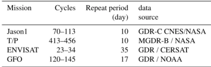
Table 1. The altimetric mission, data source and repeat cycle of each mission used for computing DOT.
Mission Cycles Repeat period data (day) source
Jason1 70–113 10 GDR-C CNES/NASA T/P 413–456 10 MGDR-B / NASA ENVISAT 23–34 35 GDR / CERSAT GFO 120–145 17 GDR / NOAA
advantages. First, it avoids any initial gridding which always implies an undesirable smoothing that is difficult to control. Second, the original sea surface heights observed along the ground tracks can be used with their high sampling rate. Fi-nally, the method treats individual profiles and consequently results in estimates of instantaneous DOT profiles. It is then straightforward to use these DOT profiles in order to generate any temporal mean representing the DOT for a specific pe-riod of time. In this paper, instantaneous multi-mission DOT profiles are used to generate a time series of ten day DOT snapshots.
The difficulty in the profile approach is to ensure the con-sistent filtering ofhandN. Let 2-D[ ]be a two-dimensional filter operator, determined by the spectral properties of the geoid. A Gauss-type Jekeli-Wahr filter (Jekeli, 1981; Wahr et al., 1998) is used here as this filter has neither side lobes in the spectral domain nor in the spatial domain. Instead of Eq. (1), the DOT should be derived by applying the 2-D filter DOT=2-D[h−NSAT] =2-D[h] −2-D[NSAT], (2) whereNSATdenotes the geoid heights from the satellite only gravity field. As h is not a two dimensional quantity, but available only along track profiles, only a one-dimensional filtering 1-D[h]can be applied. In order to account for the systematic differences between one- and two-dimensional filtering, the identity
2-D[h] =1-D[h] +2-D[h] −1-D[h]
≈1-D[h] +2-D[NHR] −1-D[NHR], (3) is used and approximated by applying the last two filter op-erations to an ultra-high resolution geoid, denoted byNHR, derived from the EGM2008 (Pavlis et al., 2008), expanded in spherical harmonics up to degree and order 2190. Com-bining Eqs. (2) and (3) and re-ordering the filter operations give
DOT=1-D[h−NHR] +δPG, (4)
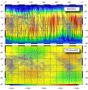
Fig. 1. Pre-Geoid corrections for GOCO01s and ITG-Grace03s gravity fields for Jekeli-Wahr filter with half width of 241.7 km.
from EGM2008 performed for the along track sequence of observation points, plus the correctionδPG evaluated at the same points. Equation (4) seems to contradict the principle discussed below Eq. (1): to subtract geoid heights of satellite only models. EGM2008, used to computeNHRin Eq. (4), is a hybrid model, based on marine gravity that in turn was derived from altimetry. Note, however,NHRwas introduced in Eq. (3) in order to compensate the systematic differences between one- and two-dimensional filtering. By re-ordering the apparently wrong geoid in Eq. (4) is compensated by the pre-geoid correction that represents the filtered difference be-tween satellite-only and high-resolution geoid.
The magnitude of the pgeoid correction is small and re-mains below a few millimetres. This is illustrated by the two panels of Fig. 1 showing for a filter length of 241 km the geo-graphical pattern ofδPGcomputed for ITG-Grace03S (lower panel) and GOCO01S (upper panel). For ITG-Grace03S the
δPGvalues are even smaller than for GOCO01S. This is due to the fact that ITG-Grace03S has been used to construct the low degree part of EGM2008 (Pavlis et al., 2008). TheδPG
values for GOCO01S exhibit some systematic differences. As GOCO01S is expected to provide a much better spatial resolution, filter operations with smaller filter length of 121 and 97 km were applied to GOCO01S only. As can be seen in Fig. 2, the magnitude ofδPGis inversely proportional to the filter length. The shorter the low-pass filter is the more details of high resolution geoid are passing the filter opera-tion.
The results of the profile approach described thus far are instantaneous DOT profiles. The sequence of ten day DOTs
Fig. 2.Pre-Geoid corrections for GOCO01s gravity field and Jekeli-Wahr filter with half width of 121 and 97 km.
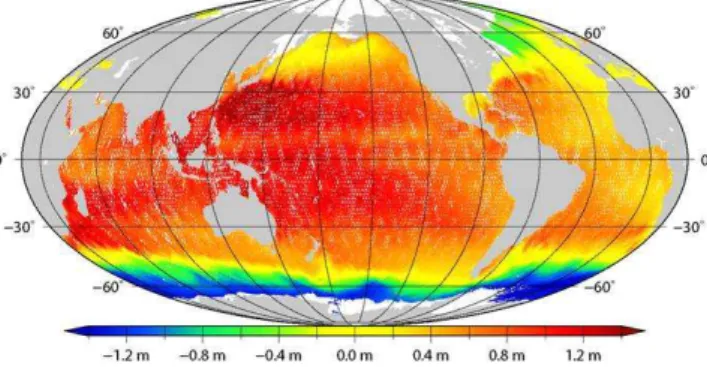
used for the assimilation are generated by linear interpola-tion onto the finite element mesh of the ocean model. This is done using distance dependent weighted mean of values from profiles lying in the cell near grid nodes. Figure 3 shows the snapshot of the multi-mission DOT computed for ten days using the filter length of 121 km. All measurements lying within a ten day period were used. Therefore, the exact time in which measurements were made was not taken into account. Figure 3 shows the lack of data (white region) in the Southern Ocean where the ice covered area drifts zonally with the seasonal cycle so that the significant part of the sur-face appears to be ice-covered at least for some time during the year. In addition, radar altimetry suffers from system-atic errors in estimating the sea state bias, an effect causing elongated radar distances in the presence of waves (Stam-mer et al., 2007; Chelton and Coauthors, 2001). This is par-ticularly critical for the Southern Oceans with rather strong winds and large waves. The Weddell Sea is without any data coverage. Further data gaps that are seen in ten day estimates of DOT result from the interpolation of the altimetry profiles to the model grid, with an area of influence of 2◦×2◦. This interpolation is kept as local as possible to avoid any addi-tional filtering of the data. The described procedure produces for every 10 days maps of DOT. The mean over 10 day maps was calculated in order to investigate the information content of these data sets.
Fig. 3.DOT from TOPEX, Jason-1, GFO, and ENVISAT obtained from data within ten day interval around 25 April 2004 and geoid from GOCO1s model. The profile approach filtering was applied using Jekeli-Wahr filter with half width of 121 km.
subpolar and mid latitude large scale gyres in both hemi-spheres. At this high resolution not only large scale but also smaller scales features of the circulation like the Labrador Current are visible. Pronounced patterns of the Antarctic Cir-cumpolar Current (ACC) stand out. Separation and merging of fronts can be observed. The result of GOCO1s model fil-tered with a half width of 241 km was compared to the results using ITG-Grace03s. As can been seen in Fig. 5 where the difference between two mean fields is shown; these are al-most identical. Small differences that do not exceed 0.5 cm can be still noted (see Fig. 5). In Fig. 5 also the differ-ences between geodetic DOTs filtered using different filter lengths are plotted. Filtering with the smaller half widths al-low many more details to remain in both altimetric and grav-ity field data. In particular, the main differences between the DOTs can be noted in the areas of strong currents, for ex-ample Gulf Stream, which now become much sharper. The differences are large if one compares results obtained by fil-tering with half widths of 241 km and 121 km (see Fig. 5 upper right) and to a lesser extent visible in the difference between 121 km and 97 km filtered results (lower left). The difference between the mean DOTs obtained as result of the filtering between 97 km (lower left) and 81 km on the other hand seems to be dominated by the noise. Further improve-ments are expected for these half widths once a full year of GOCE data are used instead of only two months which were available when this manuscript was prepared.
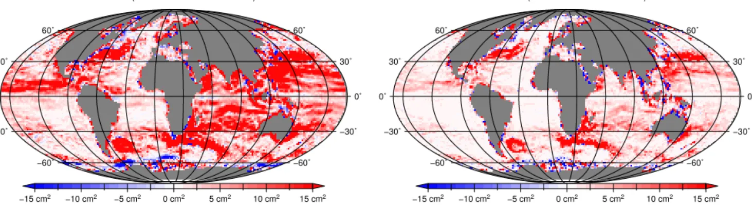
Therefore, the effect of filtering is to smear out the gra-dient resulting in weaker and less well defined estimates of the ocean currents. The filtered satellite data starting with half width of 121 km shows fine space scales that were pre-viously poorly resolved with a width of 241 km. However, also the time variability of the data sets are attenuated as a result of spatial filtering. Increase in resolution of the DOT accompanies the increase in the variability. In Fig. 6 increase in temporal variance is shown by the change of the filter length from 241 km to 121 km to 97 km. The figure shows
MDOT2004 180
−60˚ −60˚
−30˚ −30˚
0˚ 0˚
30˚ 30˚
60˚ 60˚
−1.5
−1−0.5
−0.5
0 0
0.5
0.5
1
1 1
−1.5 m −1.0 m −0.5 m 0.0 m 0.5 m 1.0 m 1.5 m
Fig. 4. Mean DOT obtained using geodetic approach with Jekeli-Wahr filter with half width of 81 km and GOCO1s geoid that com-bines GRACE and GOCE gravity data.
the increase of the signal variance of sequences of ten day DOT grids by decrease of the filter lengths. The most sig-nificant changes occur in the change of the filter length from 241 km to 121 km. The further reduction of the filter length leads to significant increase of the variances in the areas of significant variability of sea surface e.g. Gulf and Kuroshio streams. This is the result of smaller filter lengths resolving finer space scales. The apparent dilution of variance in polar and coastal areas can be explain by the better performance of the filter with the small filter length near the critical areas e.g. coast or sea ice boundaries.
3.2 Argo data set
For the validation of the results of the assimilation of DOT in Southern Atlantic, we use the Argo data set (http://www. argo.ucsd.edu, http://argo.jcommops.org). Since 1999, more than 200 Argo floats were deployed in the vicinity of the Weddell Gyre. These floats drift with the ocean currents at typically 800 m depth, collecting vertical profiles of temper-ature and salinity between 2000 m depth and the sea surface every 10 days. A quality control for temperature and salin-ity was applied according to Argo standards. The additional delayed mode quality control for salinity was performed as described in Owens and Wong (2009), i.e. comparing the float data with high quality reference CTD data (climatol-ogy). These comparisons are made on deep isotherms and assume that the temperature sensor of the float is stable and that salinity on deep isotherms is steady and uniform. The accuracy of the float data is better than 0.01◦C in
temper-ature and 0.01 in salinity. The floats are modified with ice sensing algorithm, and have RAFOS tracking allowing them to operate during winter (Klatt et al., 2007).
GOCO01s JW241.6667km − ITG−Grace03s
−60˚ −60˚
−30˚ −30˚
0˚ 0˚
30˚ 30˚
60˚ 60˚
−1.0 cm −0.5 cm 0.0 cm 0.5 cm 1.0 cm
GOCO01s (JW 120.8333km − 241.6667km)
−60˚ −60˚
−30˚ −30˚
0˚ 0˚
30˚ 30˚
60˚ 60˚
−6 cm −4 cm −2 cm 0 cm 2 cm 4 cm 6 cm
GOCO01s (JW 96.6667km − 120.8333km)
−60˚ −60˚
−30˚ −30˚
0˚ 0˚
30˚ 30˚
60˚ 60˚
−1.0 cm −0.5 cm 0.0 cm 0.5 cm 1.0 cm
GOCO01s (JW 80.5556km − 96.6667km)
−60˚ −60˚
−30˚ −30˚
0˚ 0˚
30˚ 30˚
60˚ 60˚
−1.0 cm −0.5 cm 0.0 cm 0.5 cm 1.0 cm
Fig. 5.The difference between mean geodetic DOTs obtained from GRACE data only and by combining GRACE and GOCE gravity data
with both filtered using Jekeli-Wahr filter with half width of 241 km (upper left). The difference between geodetic DOTs obtained combining GRACE and GOCE gravity data filtered with half width of 241 km and 121 km (upper right), filtered with half width of 121 km and 97 km (lower left), filtered with half width of 97 km and 81 km (lower right). Note, color scale of the plots is different.
GOCO01s (JW 120.8333km − 241.6667km)
−60˚ −60˚
−30˚ −30˚
0˚ 0˚
30˚ 30˚
60˚ 60˚
−15 cm2 −10 cm2 −5 cm2 0 cm2 5 cm2 10 cm2 15 cm2
GOCO01s (JW 96.6667km − 120.8333km)
−60˚ −60˚
−30˚ −30˚
0˚ 0˚
30˚ 30˚
60˚ 60˚
−15 cm2 −10 cm2 −5 cm2 0 cm2 5 cm2 10 cm2 15 cm2
Fig. 6. Difference in temporal variance for 2004 between half width 241 km and 121 km filtering (left), between half width 121 km and 97 km (right).
the last Argos fix from the previous cycle and dividing each underwater displacement by its corresponding exact duration (Nunez-Riboni et al., 2005). The velocities were averaged into 1.5◦ longitude by 1◦ latitude bins. A simple low-pass filter (calculating the average of a bin and all of its eight im-mediate neighbors) was applied in each bin.
In Fig. 7, locations of the Argo floats used for this calcula-tion are plotted. Differences in the regional coverage of the data that contribute to the composite can be noted. The Wed-dell gyre flow and in-situ temperature at 800 m are estimated
from Argo data covering the period from 1999 to 2010. They are depicted in Fig. 13 for comparison with results of ocean modeling.
Fig. 7.Argo data locations used to make a composite.
3.3 Satellite-tracked drifting buoys
The Global Drifter Program of NOAA and AOML collects satellite-tracked drifting buoys (“drifter”) measurements of upper ocean currents and sea surface temperature (SST). At www.aoml.noaa.gov/envids a large set of data from Febru-ary 1979 to December 2010, covering almost all the sea sur-face, are available (Lumpkin and Garraffo, 2005). In this study, as second independent data set for validation, sea sur-face temperature measured by drifting buoys is used. The SST data is for the area of Drake Passage, 70◦S to 40◦S and
70◦W to 20◦W, and for the time period from 1992 to 2010.
4 Assimilation of DOT data
4.1 Data assimilation experiments
The details of the data assimilation algorithm for the geode-tic DOT obtained using GRACE data and altimetric measure-ments are described in Janji´c et al. (2011a,b). In this section, we focus on modifications to the algorithm that need to be done in order to take into account higher resolution data. Fur-ther, we describe the assimilation scheme depending on the data and compare differences in the results of assimilation.
Four experiments were performed for the period between January 2004 and December 2004. These experiments were free model run, i.e. a model integration within the chosen time period without data assimilation and three experiments with assimilation of data filtered using Jekeli-Wahr filter with half widths of 241 km, 121 km and 97 km. These experi-ments will be labeled A241, A121 and A97 respectively. For assimilation experiments, time varying DOT data are assim-ilated every 10 days. The data assimilation scheme corrects all the ocean fields, although only geodetic DOT is assimi-lated. A diagonal observation error covariance matrix is used with 5 cm STD for experiment A241 and A121 and 7 cm STD for experiment A97. The error variance includes the errors of altimetry and geoid data and mapping errors as well as the effects of cross-correlations introduced by the interpo-lation (Janji´c and Cohn, 2006).
We use the domain localized singular evolutive interpo-lated Kalman filter (SEIK) algorithm (Pham et al., 1998; Pham, 2001; Nerger et al., 2006) as implemented within the parallel data assimilation framework (PDAF, Nerger et al., 2005). We update the full model state, consisting of tem-perature, salinity, SSH, and velocity fields. The SEIK algo-rithm is used together with the method of weighting obser-vations proposed by Hunt et al. (2007). During the assimi-lation, the analysis of the full ocean state is carried out for each column of the model separately. The update of each column is assumed to depend only on observations within a specified influence region. In addition, the observations are weighted as a function of their distance from the point at which the assimilation is made. After obtaining the anal-ysis the new ensemble is generated by second order exact resampling (Pham, 2001). Each ensemble is propagated with FEOM ocean model for 10 days producing the forecast of ensembles. Forecast of all model variables is obtained by averaging over the ensemble members. This forecasted field together with the next 10 day DOT map is used for obtaining the new analysis.
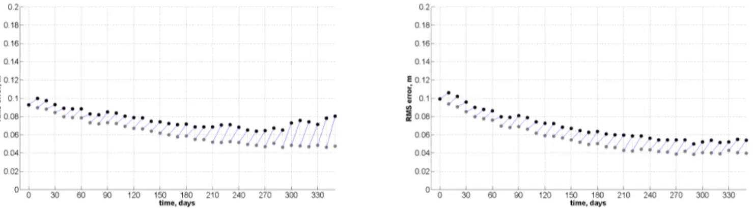
In Janji´c et al. (2011a) it was shown that (a) the optimal influence region is a circle with a radius of 900 km for obser-vations that are filtered with half width of 241 km and (b) that optimal covariance for localization of ensemble Kalman fil-ter algorithm approximates well a Gaussian with length scale of 246 km. For the data filtered up to 121 km, experiments were performed using the same specification, as well as a lo-calization function with length scale of 123 km. For these two experiments, Fig. 8 shows the 10 day time evolution of the RMS error of the SSH for analysis and forecast com-pared to the data assimilated over the entire ocean. Further experiments with different length scale of localization func-tion confirmed that the length scale of 123 km is optimal for observations that are filtered with half width of 121 km. As seen in Fig. 8 the analysis results are closer to data than pre-diction. However the prediction drifts away from the analysis only moderately. The RMS error of the inferred DOT could be reduced from 16 cm (for the model only experiment com-pared to the geodetic DOT) to 4 cm for analysis and 5 cm for the prediction if proper length scale, depending on the data that is assimilated, is used. Accordingly, the length scale of localization function was chosen to have 98.4 km in experi-ment A97.
Fig. 8. Evolution of RMS error of SSH for the world ocean. The black bullets represent the sequence of 10-day model forecasts, while gray bullets correspond to the analysis. RMS error for assimilation of data filtered up to half width of 121 km and localization function that correspond to Gaussian with length scale 246 km (left). RMS error for assimilation of the same data with localization function that corresponds to Gaussian with length scale 123 km (right).
Fig. 9. The impact of increasing the resolution in the DOT data. Depicted is the difference between mean oceanic DOTs as a result of A241 and A121 experiments (left). The same for A121 and A97 experiments (right). Frontal positions of Orsi et al. (1995) are depicted with black lines. Units are m.
4.2 Results of global assimilation of DOT
The DOT resulting from the data assimilation experiments reflects the impacts of the geodetic DOT data used, of the forcing, and of the physical and dynamical properties of the ocean model. In order to investigate the ability of the data assimilation scheme to incorporate the higher resolution data into the model, the difference between the mean analysis ob-tained as a result of assimilation of different resolution of data is considered. Figure 9 shows the difference between mean oceanic DOTs of A241 and A121 experiments as well as the difference for A121 and A97 experiments. We notice similar patterns and magnitudes as already shown in Fig. 5 for data only fields. The increase in resolution of data from the half width of 241 to 121 km modifies the DOT fields with the differences that can exceed 10 cm, while the changes from the half width of 121 to 97 km are smaller and on the or-der of few centimeters. Corresponding results for SST show differences that are in the range of 0.5◦C between the anal-ysis results. For SST the major effects can be seen in the Southern Ocean, equatorial, as well as in the western bound-ary currents regions. The increase in resolution in sea surface
salinity results is less pronounced compared to DOT or SST. Salinity, though, in the most active areas of the global ocean is effected by increase of resolution of DOT data as the other fields.
Finally, the variability is larger for the data less filtered, and therefore it is also more difficult to be reproduced by the model. Although data assimilation increases the variability of free model depending on the resolution of the data assim-ilated, all experiments show variability below the variability presented for DOT data in Fig. 6.
4.3 Results of global assimilation of DOT in Southern
Ocean
Fig. 10. The difference between mean analysis DOT of A241 and free model (left) and of A241 and A97 (right). The black lines are the Subantarctic, Polar and southern boundary of ACC fronts computed from in-situ measurements (Orsi et al., 1995). Units are m.
135
oW
90
o
W
45
o
W
0
o45
oE
90
o
E
135
o
E
180
oW
70
oS
50
oS
−1.5
−1
−0.5
0
0.5
1
135
o
W
90
o
W
45
o
W
0
o45
o
E
90
o
E
135
o
E
180
oW
70
oS
50
oS
−1.5
−1
−0.5
0
0.5
1
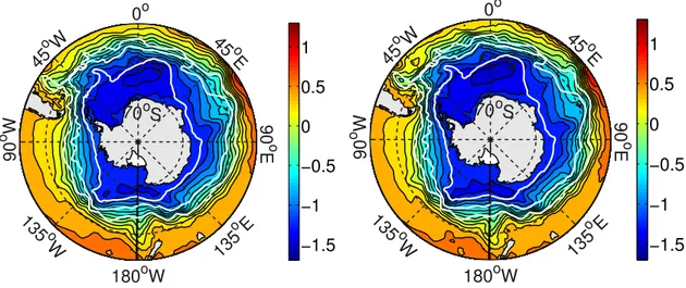
Fig. 11.The mean analysis DOT as result of A241 (left) and A97 (right) experiments for Southern Ocean. The white lines are the Subantarctic and Polar fronts and southern boundary of ACC computed from in-situ measurements (Orsi et al., 1995). Units are m.
70◦E and 120◦E, as well as at 140◦W. These locations are
characterized by strong eddy activity. Higher resolution of GOCE data does not significantly decrease the differences. Its biggest impact is to sharpen the oceanic fronts.
Modification from the DOT of the free model to the DOT of A241 experiment is presented in Fig. 10 for Southern Ocean (left panel). Changes to the large scale flow field of a numerical model are significant, and as we will see later already the inclusion of the low resolution DOT improves the free model run. On the other hand, the difference be-tween DOTs from experiments A241 and A97 are concen-trated in the area of strong currents (right panel Fig. 10). Superimposed on the figures are location of the Subantartic and Polar fronts and southern boundary of ACC as estimated from historical hydrographic station data (Orsi et al., 1995).
Consistent with the increase in the resolution of the data, data assimilation results show that higher degree of DOTs further modify the areas of high variability. The mean DOT obtained as the result of analysis in the Southern Ocean for A241 and A97 experiment are shown in Fig. 11. Sokolov and Rintoul (2009) argue that the frontal location can be determined by the contour lines of SSH. In Fig. 11 the contour lines of SSH follow better the Orsi et al. (1995) front locations in Conflu-ence Area of South Atlantic (East of the Argentine) where the turning of the Subantartic front now coincides with the estimates of location of this front by Orsi et al. (1995).
70
oW 60
oW 50oW 40oW 30o
W 20o
W 66 oS 60 oS 54 oS 48 oS 42 oS 0 5 10 15
20 70
oW 60
oW 50oW 40oW 30o
W 20o
W 66 oS 60 oS 54 oS 48 oS 42 oS 0 5 10 15 20
Fig. 12.The SST from surface drifter data in Drake passage area (left) and A97 experiment (right). The black lines are the Subantarctic and Polar fronts and southern boundary of ACC computed from in-situ measurements (Orsi et al., 1995). Units are Celsius.
50
oW
25 oW 0o 25o
E 50 o E 78 oS 72 oS 66 oS 60 oS 54 oS 50 oW 25 oW 0o 25o
E 50 o E 78 oS 72 oS 66 oS 60 oS 54 oS 0.5 1 1.5 2 50 oW
25oW 0
o
25oE
50 o E 78 oS 72 oS 66 oS 60 oS 54 oS 50 oW
25oW 0
o
25oE
50 o E 78 oS 72 oS 66 oS 60 oS 54 oS 0.5 1 1.5 2 50 oW
25oW 0
o
25oE
50 o E 78 oS 72 oS 66 oS 60 oS 54 oS 50 oW
25oW 0
o
25oE
50 o E 78 oS 72 oS 66 oS 60 oS 54 oS 0.5 1 1.5 2
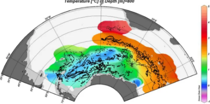
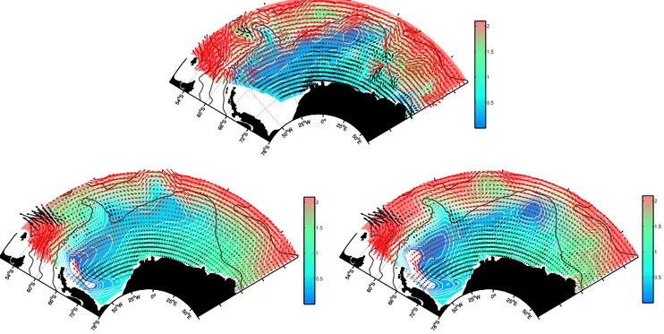
Fig. 13. The Weddell gyre flow and in-situ temperature at 800 m depth derived from 206 ice-compatible vertically profiling floats (Klatt et al., 2007) between 1999 and 2010 (top) following (Fahrbach et al., 2011). Corresponding figure for free model (bottom left) and A97 experiment (bottom right). Red and black arrows indicate eastward and westward currents, respectively. Frontal positions of Orsi et al. (1995) are depicted with black lines.
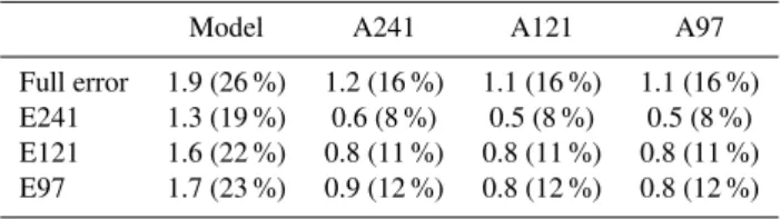
illustrated in Fig. 12. For the area with good drifter coverage, 60◦S to 42◦S and 58◦W to 30◦W, the RMS error to SST drifter data was almost half once DOT data are assimilated. The errors as well as percentage of the erroneous signal are given in Table 2 for all four experiments. The improvement with different data resolution for SST is only 0.1◦C, from A241 to A97 experiments. Both model SST results as well as drifter data can be filtered in order to produce the com-parable signal. This has been done using the spatial Gauss filter corresponding to the resolution of the DOT data, i.e.
25oW 0 o 25o E 78 oS 72 oS 66 oS 60 oS 54 oS
25oW 0
o 25o E 78 oS 72 oS 66 oS 60 oS 54 oS −0.6 −0.6 −0.4 −0.4 −0.4 −0.4 −0.4 −0.4 −0.2 −0.2 −0.2 −0.2 −0.2 −0.2 0 0 0 0 0 0.2 0.2 0.2 0.2 0.2 0.2 0.2 0.2 0.4 0.4 0.4 0.4 0.4 −0.6 0.4 0.4 0 −0.4 0.4 0 50
oW 50
o E −0.4 −0.2 −0.2 0 0 −0.6 −0.4 −0.2 0 0.2 0.4 25
oW 0o 25 o E 78 oS 72 oS 66 oS 60 oS 54 oS 25
oW 0o 25 o E 78 oS 72 oS 66 oS 60 oS 54 oS −0.6 −0.6 −0.6 −0.6 −0.4 −0.4 −0.2 −0.2 −0.2 −0.2 −0.2 −0.2−0.2 0 0 0 0 0 0 0.2 0.2 0.2 0.2 0.2 0.2 0 0 0 0 0.2 0.2 0.2 0.4 0.4 0.4 −0.4 0 −0.2
0.4 −0.6 0.2 −0.4
0.4
0
50
oW 50
o E −0.6 0.4 0.4 −0.6 −0.4 −0.2 0 0.2 0.4 25
oW 0o
25o E 78 oS 72 oS 66 oS 60 oS 54 oS 25
oW 0o
25o E 78 oS 72 oS 66 oS 60 oS 54 oS −0.6 −0.6 −0.6 −0.6 −0.4 −0.4 −0.4 −0.4 −0.4 −0.2 −0.2 −0.2 −0.2 −0.2 −0.2 0 0 0 0 0 0 0 0 0.2 0.2 0.2 0.2 0.2 0.2 0.2 0.2 0.4 0.4 0.4 0.4 −0.2 0.2 0.4 −0.2 0.2 −0.2 0.4 0 0 0 50
oW 50
o E −0.2 −0.6 −0.4 −0.2 0 0.2 0.4 25
oW 0o
25o E 78 oS 72 oS 66 oS 60 oS 54 oS 25
oW 0o
25o E 78 oS 72 oS 66 oS 60 oS 54
oS −0.6
−0.4 −0.4 −0.4 −0.4 −0.2 −0.2 −0.2 −0.2 −0.2 −0.2 0 0 0 0 0 0 0 0 0 0.2 0.2 0.2 0.2 0.2 0.2 0.4 0.4 0.4 0.4 0.4 −0.2 0.2 0.2 0.2 0 0 0 50
oW 50o
E −0.6 −0.4 −0.2 0 0.2 0.4
Fig. 14.The difference between in-situ temperature at 800 m depth from free model (upper left), A241 (upper right), A121 (lower left) and A97 (lower right) experiments and Argo composite, respectively. Frontal positions of Orsi et al. (1995) are depicted with black lines.
Table 2.SST RMS error values from four experiments compared to surface drifter data in Drake passage area. Units are degree Celsius. E241, E121 and E97 indicate the RMS error values when both SSTs are first filtered using Gauss spatial filter with half width of 241, 121 and 97 km, respectively. In parenthesis percentage of error for this area is given. Percentage is calculated by normalizing with RMS value of the drifter SST data or appropriately filtered drifter data in case of E241, E121 and E97.
Model A241 A121 A97 Full error 1.9 (26 %) 1.2 (16 %) 1.1 (16 %) 1.1 (16 %) E241 1.3 (19 %) 0.6 (8 %) 0.5 (8 %) 0.5 (8 %) E121 1.6 (22 %) 0.8 (11 %) 0.8 (11 %) 0.8 (11 %) E97 1.7 (23 %) 0.9 (12 %) 0.8 (12 %) 0.8 (12 %)
It is interesting to compare the assimilation results for sub-surface temperature in the area which is only partially ob-served by altimetry, namely Weddell Sea. For this com-parison we use the independent Argo data set (presented in Sect. 3.2) to show the impact of assimilation of global DOT. At about 30◦E, both temperature and flow field ob-tained from Argo data (see top panel of Fig. 13) show clearly the southward spreading of waters influenced by the ACC, resulting in an intrusion of warm water masses with tem-peratures of about 1◦C into Antarctic waters. From about
60◦S southward, these waters spread to the west as part of
the southern branch of the Weddell Gyre. Their subsequent transformation into deep and bottom water feeds the global thermohaline circulation. Additional southward float dis-placements are just about visible to the east of Conrad Rise at about 50◦E. Possibly, warmer waters from the north are entrained here into the Weddell Gyre as well, which would be consistent with Park and Gamb´eroni (1995), who place the boundary of the Weddell Gyre as far east as 60◦E near the Kerguelen Plateau. In conjunction with the recirculation of the southern branch of the Weddell Gyre in the vicinity of the Greenwich Meridian and the temperature minimum at (58◦S, 10◦E), this observation supports the double cell
structure of the Weddell Gyre as suggested by Beckmann et al. (1999). The Subantartic and Polar fronts and southern boundary of ACC as estimated from historical station data (Orsi et al., 1995) are superimposed on the Fig. 13. It is interesting to note very good agreement between southern boundary of ACC as estimated by Orsi et al. (1995) with in situ data available at that time and the new Argo composite results.
The spatial distribution, similar as presented in the Fig. 13 for the results of assimilation of 97 km DOT data, appears al-ready with assimilation of data filtered to 241 km. In Fig. 14 the difference in temperature at 800 m depth to Argo compos-ite is plotted for four experiments. Differences between tem-perature and Argo composite decrease with increased reso-lution. The area in between southern boundary of ACC and Polar front is represented better with use of the data assimi-lation and with use of higher resolution data. Warmer water is entrained between the front lines as result of assimilation in the area between 30◦W and 0◦, for example. Similarly with higher resolution data, area 25◦E to 50◦E and north of 54◦S shows better agreement to the Argo data. Minima at 58◦S at 10◦E in the Argo data is seen in the assimilation of global DOT results, however more to the East than ob-served. Temperature in the area between 25◦W to 25◦E is
now significantly closer to that observed by Argo. Also, wa-ter masses characwa-terized by lower than observed temperature west of 30◦W are closer to observed values with higher
res-olution data. Unfortunately the changes to the velocity field are very modest at 800 m level. Also the temperature field south of 66◦S still is warmer than observed by Argo data.
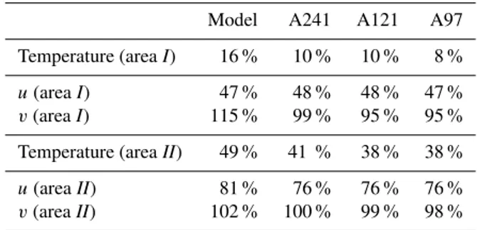
RMS values for free model and for the three assimilation experiments, compared to Argo composite at 800 m are cal-culated. Use of data assimilation decreased the RMS differ-ences for temperature and slightly for velocities once the data filtered to half width of 241 km are used. Further improve-ments can be noted when data with higher spectral resolu-tion is assimilated. The RMS differences for A97 experiment are 0.35◦C for temperature and 3.4, 2.4 cm s−1for velocity, north of 60◦S values are 0.22◦C, 4 and 2.8 cm s−1. In Ta-ble 3 two areas are chosen corresponding to the coverage of the Argo data (Fig. 7): areaIis from 55◦S to 50◦S and in
be-tween 0◦to 60◦E, and areaIIsouth of 55◦S and from 40◦W
to 30◦E. The area II is without DOT data coverage. Simi-larly as for SST the largest reduction in error at 800 m depth is from free model run to A241. Additional reduction of the error due to the higher resolution of DOT data is not as large. In area II the errors are still large after assimilation, but the decrease in the error follows the increase in resolution. The calculated RMS errors for the velocity fields at 800 m depth remain large for both areas considered.
So far comparison of the four experiments with indepen-dent data has been done for the mean fields. Finally, the com-parison of the potential temperature for all depths and for all Argo profiles south of 40◦S for December 2004 is done
(fig-ure not shown). A decrease in the mean error with increased resolution occurs. The decrease is from−0.3,−0.22,−0.17, to−0.09 for free model, A241, A121 and A97. The STD follows 1.1, 0.8, 0.6 to 0.95 respectively. The increase in the STD from A121 to A97 experiment is consistent with increase in noise of the DOT data for experiment A97.
Table 3.Normalized RMS error values from four experiments com-pared to the Argo data for the areasIandIIat 800 m depth. RMS errors are normalized with RMS value of Argo measurements and given as percentage.
Model A241 A121 A97
Temperature (areaI) 16 % 10 % 10 % 8 %
u(areaI) 47 % 48 % 48 % 47 %
v(areaI) 115 % 99 % 95 % 95 %
Temperature (areaII) 49 % 41 % 38 % 38 %
u(areaII) 81 % 76 % 76 % 76 %
v(areaII) 102 % 100 % 99 % 98 %
5 Conclusions
Geodetic DOT with much finer space scales, that were pre-viously poorly resolved, is obtained by combining GRACE and GOCE gravity field data. The resolution of the sea sur-face height data is still higher than the resolution of the geoid, and requires filtering in order to obtain spectrally consistent fields. In our study we used the profile approach filtering to obtain 10 day maps of DOT. Spatial filtering, in addition to removing noise also attenuates the gradients of DOT. By including two months of GOCE data the profile approach fil-tering was able to remove the noise and preserve as far as possible the oceanographic content of the DOT. The mean obtained by averaging 10 day geodetic estimates of DOT shows fine space scale structures that are particularly visi-ble in the areas of strong currents. Further improvement in geodetic data sets is expected once more months of GOCE data become available.
were not used for assimilation and lie outside the area cov-ered by altimetry in the Southern Ocean.
Appendix A
Mission specific corrections
First homogenization of the altimeter data was performed. This means that as far as possible the best mission specific corrections were applied and common geophysical models for the mean ocean tide models, geoid heights, and reaction of sea level to atmospheric pressure were used. For the com-putation of altimetric sea surface heights, the standard cor-rections provided with the used altimeter products (see Ta-ble 1) were applied with the following modifications:
1. for GFO the ionospheric corrections were computed from GIM ionospheric model scaled with the IRI model (Iijima et al., 1999);
2. all corrections described in Schrama et al. (2000) were applied to the ERS-1/2 data sets;
3. the orbit data of ERS-1/2 was replaced by DEOS precise orbits (Scharroo and Visser, 1998);
4. the GDR ENVISAT orbits were replaced by ESA orbits of GDR-C standards;
5. for Jason1 the radiometer wet troposphere correction are replaced using replacement product provided by Jet Propulsion Laboratory (JPL) (S. Desai, personal com-munication, 2009);
6. for the sea state bias of TOPEX, the model of Chambers et al. (2003) was used;
7. the orbits of TOPEX and Jason-1 missions were re-placed by Lemoine et al. (2010);
8. for Jason-1, TOPEX/Poseidon and ENVISAT, the dual frequency ionospheric corrections were smoothed by means of median filter with the filter length of 20 sec; 9. the TOPEX microwave radiometer are replaced using
replacement product (S. Desai, personal communica-tion, 2003);
10. for all missions the inhomogeneous inverted barometric corrections were replaced by dynamic atmospheric cor-rections which are produced by CLS Space Oceanog-raphy Division using the Mog2-D model from Legos and distributed by Aviso, with support from Cnes (http: //www.aviso.oceanobs.com/);
11. for all altimeter systems the ocean tide corrections were computed using the EOT10a (Mayer-G¨urr et al., 2012) tide model;
The second step was the multi-mission-cross-calibration. The radial error component and relative mission specific bi-ases were corrected by means of multi-mission-crossover analysis (Dettmering and Bosch, 2010).
Acknowledgements. This work has been funded under DFG
Priority Research Programme SPP 1257 “Mass Transport and Mass Distribution in the Earth System”.
Edited by: E. J. M. Delhez
References
Beckmann, A., Hellmer, H., and Timmermann, R.: A numerical model of the Weddell Sea, large-scale circulation and water mass distribution, J. Geophys. Res., 104, 23374–23391, 1999. Bingham, R. J., Haines, K., and Hughes, C. W.: Calculating the
Ocean’s Mean Dynamic Topography from a Mean Sea Surface and a Geoid, J. Atmos. Ocean. Tech., 25, 1808–1822, 2008. Chambers, D. P., Hayes, S. A., Ries, J. C., and Urban, T. J.: New
TOPEX sea state bias models and their effect on global mean sea level, J. Geophys Res., 108, 3305, doi:10.1029/2003JC001839, 2003.
Chelton, D. B., Esbensen, S. K., Schlax, M. G., Thum, N., Freilich, M. H., Wentz, F. J., Gentemann, C. L., McPhaden, M. J., and Schopf, P. S.: Observations of coupling between surface wind stress and sea surface temperature in the eastern tropical Pacific, J. Climate, 14, 1479–1498, doi:http://dx.doi.org/10.1175/1520-0442(2001)014<1479:OOCBSW>2.0.CO;2, 2011.
Danilov, S., Kivman, G., and Schr¨oter, J.: A finite-element ocean model: principles and evaluation, Ocean Model., 6, 125–150, 2004.
Dettmering, D. and Bosch, W.: Global Calibration of Jason-2 by Multi-Mission Crossover Analysis, Mar. Geodesy, 33, 150–161, doi:10.1080/01490419.2010.487779, 2010.
Fahrbach, E.: Die Expedition ANTARKTIS XV/4 des Forschungss-chiffes POLARSTERN 1998, [28. M¨arz 1998–23.‘Mai 1998, Punta Arenas – Kapstadt]=The expedition ANTARKTIS XV/4 of the research vessel POLARSTERN in 1998, Berichte zur Polar- und Meeresforschung=Reports on polar and marine re-search 314, Alfred Wegener Institute for Polar and Marine Re-search, 1999.
Fahrbach, E. and de Baar, H.: The expedition of the research ves-sel POLARSTERN to the Antarctic in 2008 (ANT-XXIV/3), Berichte zur Polar- und Meeresforschung=Reports on polar and marine research 606, edited by: Fahrbach, E. and de Baar, H., Alfred Wegener Institute for Polar and Marine Research, 2010. Fahrbach, E. and Naggar, S. E.: Die Expeditionen ANTARKTIS
XVI/1-2 des Forschungsschiffes POLARSTERN 1998/1999= The expeditions ANTARKTIS XVI/1-2 of the research vessel POLARSTERN in 1998/1999, Berichte zur Polar- und Meeres-forschung=Reports on polar and marine research 380, Alfred Wegener Institute for Polar and Marine Research, 2001. Fahrbach, E., Fuetterer, D. K., and Naggar, S. E. D. E.: Die
Polar- und Meeresforschung=Reports on polar and marine re-search 445, Alfred Wegener Institute for Polar and Marine Re-search, 2003.
Fahrbach, E., Hoppema, M., Rohardt, G., Boebel, O., Klatt, O., and Wisotzki, A.: Warming of deep and abyssal water masses along the Greenwich meridian on decadal time scales: The Wed-dell gyre as a heat buffer, Deep-Sea Res. Pt. II, 58, 2509–2523, doi10.1016/j.dsr2.2011.06.007, 2011.
Gouretski, V. V. and Koltermann, K. P.: WOCE Global graphic Climatology, Bundesamt f¨ur Seeschifffahrt und Hydro-graphie, Hamburg und Rostock, Germany, 2004.
Griesel, A., Gille, S. T., and Mazloff, M.: Using dynamic ocean to-pography to probe the southern ocean circulation, Geophys. Res. Abstr., EGU2010-5565, EGU General Assembly 2010, Vienna, Austria, 2010.
Hunt, B. R., Kostelich, E. J., and Szunyogh, I.: Efficient Data As-similation for Spatiotemporal Chaos: A local Ensemble Trans-form Kalman filter, Physica D, 230, 112–126, 2007.
Iijima, B. A., Harris, I. L., Ho, C. M., Lindqwister, U. J., Mannucci, A. J., Pi, X., Reyes, M. J., Sparks, L. C., and Wilson, B. D.: Au-tomated daily process for global ionospheric total electron con-tent maps and satellite ocean ionospheric calibration based on Global Positioning System, J. Atmos. Sol.-Terr. Phys., 61, 1205– 1218, 1999.
Janji´c, T. and Cohn, S. E.: Treatment of Observation Error due to Unresolved Scales in Atmospheric Data Assimilation, Mon. Weather Rev, 134, 2900–2915, 2006.
Janji´c, T., Nerger, L., Albertella, A., Schroeter, J., and Skachko, S.: On domain localization in ensemble based Kalman filter algorithms, Mon. Weather Rev, 139, 2046–2060, doi:10.1175/2011MWR3552.1, 2011a.
Janji´c, T., Schr¨oter, J., Albertella, A., Bosch, W., Rum-mel, R., Savcenko, R., Schwabe, J., and Scheinert, M.: Assimilation of geodetic dynamic ocean topography using ensemble based Kalman filter, J. Geodynam., in press, doi:10.1016/j.jog.2011.07.001, 2011b.
Jekeli, C.: Alternative methods to smooth the earth’s gravity field, in: Dept. Geod. Sci. and Surv., Ohio State University, Columbus., rep. 327, 1981.
Klatt, O., Boebel, O., and Fahrbach, E.: A Profiling Float’s Sense of Ice, J. Atmos. Ocean Tech., 24, 1301–1308, 2007.
K¨ohl, A., Stammer, D., and Cornuelle, B.: Interannual to Decadal Changes in the ECCO Global Synthesis, J. Phys. Oceanogr., 37, 313–337, 2007.
Le Grand, P., Schrama, E. J. O., and Tournadre, J.: An inverse es-timate of the dynamic topography of the ocean, Geophys. Res. Lett., 30, 1062, doi:10.1029/2002GL014917, 2003.
Lemoine, F., Zelensky, N., D. S., Chinn, Pavlis, D., Rowlands, D., Beckley, B., Luthcke, S., Willis, P., Ziebart, M., Sibthorpe, A., Boy, J., and Luceri, V.: Towards development of a consistent orbit series for TOPEX/Poseidon, Jason-1, and Jason-2, Adv. Space Res., DORIS special issue, 46, 1513–1540, 2010. L¨ohner, R., Morgan, K., Peraire, J., and Vahdati, M.: Finite-element
flux-corrected transport (FEM-FCT) for the Euler and Navier-Stokes equations, Int. J. Numer. Meth. Fl., 7, 1093–1109, 1987. Losch, M. and Schr¨oter, J.: Estimating the circulation from
hydrog-raphy and satellite altimetry in the Southern Ocean: limitations imposed by the current geoid models, Deep-Sea Res. Pt. I, 51, 1131–1143, 2004.
Lumpkin, R. and Garraffo, Z.: Evaluating the Decomposition of Tropical Atlantic Drifter Observations, J. Atmos. Ocean. Tech., 22, 1403–1415, 2005.
Maximenko, N., Niiler, P., Rio, M.-H., Melnichenko, O., Centu-rioni, L., Chambers, D., Zlotnicki, V., and Galperin, B.: Mean dynamic topography of the ocean derived from satellite and drift-ing buoy data usdrift-ing three different techniques, J. Atmos. Ocean. Tech., 26, 1910–1919., 2009.
Mayer-G¨urr, T.: ITG-GRACE03s: The latest GRACE gravity field solution computed in Bonn, in: Presentation, Joint Grace Sc. Team and DFG SPP Meeting, Potsdam, Germany, Oct. 15, 2007, 2007.
Mayer-G¨urr, T., Savcenko, R., Bosch, W., Daras, I., Flechtner, F., and Dahle, C.: Ocean tides from satellite altimetry and GRACE, J. Geodynam., in press, doi:10.1016/j.jog.2011.10.009, 2012. Menkes, C., Boulanger, J., Busalacchi, A., Vialard, J., Delecluse, P.,
McPhaden, M., Hackert, E., and Grima, N.: Impact of TAO vs. ERS wind stresses onto simulations of the tropical Pacific Ocean during the 1993-1998 period by the OPA OGCM, in: Climate Impact of Scale Interaction for the Tropical Ocean-Atmosphere System, Vol. 13 of Euroclivar Workshop Report, 1998.
Nerger, L., Hiller, W., and Schr¨oter, J.: PDAF – The Parallel Data Assimilation Framework: Experiences with Kalman filtering, in: Use of High Performance Computing in Meteorology, Pro-ceedings of the 11. ECMWF Workshop, World Scientific, read-ing, UK, 25–29 October 2004, edited by: Zwieflhofer, W. and Mozdzynski, G., Singapore, 63–83, 2005.
Nerger, L., Danilov, S., Hiller, W., and Schr¨oter, J.: Using sea level data to constrain a finite-element primitive-equation ocean model with a local SEIK filter, Ocean Dynam., 56, 634–649, 2006. Nunez-Riboni, I., Boebel, O., Ollitrault, M., You, Y., Richardson,
P., and Davis, R.: Lagrangian Circulation of Antarctic Interme-diate Water in the subtropical South Atlantic, Deep-Sea Res. Pt. II, 52, 545–564, 2005.
Orsi, A. H., Whitworth III, T., and Nowlin Jr., W. D.: On the merid-ional extent and fronts of the Antarctic Circumpolar Current, Deep-Sea Res. Pt. I, 42, 641–673, 1995.
Owens, W. B. and Wong, A. P. S.: An improved calibration method for the drift of the conductivity sensor on autonomous CTD pro-filing floats by theta-S climatology, Deep-Sea Res. Pt. I, 56, 450– 457, 2009.
Pail, R., Goiginger, H., Schuh, W. D., H¨ock, E., Brockmann, J. M., Fecher, T., Gruber, T., Mayer-G¨urr, T., Kusche, J., J¨aggi, A., and Rieser, D.: Combined satellite gravity field model GOCO01S de-rived from GOCE and GRACE, Geophys. Res. Lett., 37, L20314, 5 pp, doi:10.1029/2010GL044906, 2010.
Pakanowski, R. and Philander, S.: Parametrization of vertical mix-ing in numerical models of tropical oceans, J. Phys. Oceanogr., 11, 1443–1451, 1981.
Park, Y.-H. and Gamb´eroni, L.: Large-scale circulation and its vari-ability in the South Indian Ocean from TOPEX/POSEIDON al-timetry, J. Geophys. Res., 100, 911–924, 1995.
Pavlis, N. K., Holmes, S. A., Kenyon, S. C., and Factor, J. K.: An Earth Gravitational Model to Degree 2160: EGM2008, Geophys. Res. Abstr., EGU2008-A-01891, EGU General Assembly 2008, Vienna, Austria, 2008.
Res., 60, 805–833, 2002.
Pham, D. T.: Stochastic methods for sequential data assimilation in strongly nonlinear systems, Mon. Weather Rev., 129, 1194– 1207, 2001.
Pham, D. T., Verron, J., and Gourdeau, L.: Singular evolutive Kalman filters for data assimilation in oceanography, C. R. Acad. Sci. Ser. II, 326, 255–260, 1998.
Rio, M.-H., Schaeffer, P., Lemoine, J.-M., and Hernandez, F.: Estimation of the ocean Mean Dynamic Topography through the combination of altimetric data, in-situ measurements and GRACE geoid: From global to regional studies, Proceedings of the GOCINA international workshop, Luxembourg, 2005. Rio, M.-H., Schaeffer, P., Moreaux, G., Lemoine, J.-M., and
Bron-ner, E.: A new mean dynamic topography comuted over the global ocean from GRACE data, altimetry and in-situ measure-ments, in: OceanObs09 Venice, poster, 2009.
Rollenhagen, K., Timmermann, R., Janji´c, T., Schroeter, J., and Danilov, S.: Assimilation of sea ice motion in a Fi-nite Element Sea Ice Model, J. Geophys. Res., 114, C05007, doi:10.1029/2008JC005067, 2009.
Scharroo, R. and Visser, P. N. A. M.: Precise orbit determination and gravity field improvement for the ERS satellites, J. Geophys Res., 103, 8113–8127, 1998.
Schrama, E., Scharroo, R., and Naeije, M.: Radar Altimeter Database System (RADS): Towards a generic multi-satellite al-timeter database system, USP-2 00, BCRS/SRON, Delft, The Netherlands, 2000.
Schr¨oder, M. and Fahrbach, E.: On the structure and the transport in the Eastern Weddell Gyre, Deep-Sea Res. Pt. II, 46, 501–527, 1999.
Schr¨oter, J., Losch, M., and Sloyan, B.: Impact of the Gravity Field and Steady-State Ocean Circulation Explorer (GOCE) mission on ocean circulation estimates 2, Volume and heat transports across hydrographic sections of unequally spaced stations, J. Geophys. Res., 107, 11–13, doi:10.1029/2000JC000647, 2002.
Sidorenko, D., Wang, Q., Danilov, S., and Schr¨oter, J.: FESOM under Coordinated Ocean-ice Reference Experiment forcing, Ocean Dynam., 61, 881–890, doi:10.1007/s10236-011-0406-7, 2011.
Skachko, S., Danilov, S., Janji´c, T., Schr¨oter, J., Sidorenko, D., Savcenko, R., and Bosch, W.: Sequential assimilation of multi-mission dynamical topography into a global finite-element ocean model, Ocean Sci., 4, 307–318, doi:10.5194/os-4-307-2008, 2008.
Sokolov, S. and Rintoul, S. R.: Circumpolar structure and distribu-tion of the Antartic Circumpolar Current Fronts: Mean circum-polar parts, J. Geophys. Res., 114, 1–19, 2009.
Stammer, D., K¨ohl, A., and Wunsch, C.: Impact of accurate Geoid fields on Estimates of the Ocean Circulation, J. Atmos. Ocean. Tech., 24, 1464–1478, 2007.
Stephens, J., Antonov, T., Boyer, T., Conkright, M. E., Locarnini, R. A., OBrien, T. D., and Garcia, H. E.: World ocean Atlas 2001, in: Temperatures, edited by: Levitus, S., NOAA Atlas NESDIS 49, US Government Printing Office, 167 pp., 2002.
Timmermann, R., Danilov, S., Schr¨oter, J., B¨oning, C., Sidorenko, D., and Rollenhagen, K.: Ocean circulation and sea ice distri-bution in a finite element global sea ice-ocean model, Ocean Model., 27, 114–129, 2009.
Wahr, J., Bryan, F., and Molenaar, M.: Time variability of the Earth’s gravity field: Hydrological and oceanic effects and their possible detection using GRACE, J. Geophys. Res., 103, 30205– 30229, 1998.
Wang, Q., Danilov, S., and Schroeter, J.: Finite element ocean circu-lation model based on triangular prismatic elements with applica-tion in studying the effect of topography representaapplica-tion, J. Geo-phys. Res., 113, C05015, 21 pp., doi:10.1029/2007JC004482, 2008.