www.ocean-sci.net/12/1179/2016/ doi:10.5194/os-12-1179-2016
© Author(s) 2016. CC Attribution 3.0 License.
Sub-basin-scale sea level budgets from satellite altimetry, Argo floats
and satellite gravimetry: a case study in the North Atlantic Ocean
Marcel Kleinherenbrink, Riccardo Riva, and Yu Sun
Department of Geoscience and Remote Sensing, Delft University of Technology, P.O. Box 5048, 2600 GA Delft, the Netherlands
Correspondence to:Marcel Kleinherenbrink (m.kleinherenbrink@tudelft.nl) Received: 22 June 2016 – Published in Ocean Sci. Discuss.: 6 July 2016
Revised: 25 October 2016 – Accepted: 26 October 2016 – Published: 15 November 2016
Abstract.In this study, for the first time, an attempt is made to close the sea level budget on a sub-basin scale in terms of trend and amplitude of the annual cycle. We also compare the residual time series after removing the trend, the semi-annual and the semi-annual signals. To obtain errors for altimetry and Argo, full variance–covariance matrices are computed using correlation functions and their errors are fully prop-agated. For altimetry, we apply a geographically dependent intermission bias (Ablain et al., 2015), which leads to differ-ences in trends up to 0.8 mm yr−1. Since Argo float measure-ments are non-homogeneously spaced, steric sea levels are first objectively interpolated onto a grid before averaging. For the Gravity Recovery And Climate Experiment (GRACE), gravity fields full variance–covariance matrices are used to propagate errors and statistically filter the gravity fields. We use four different filtered gravity field solutions and deter-mine which post-processing strategy is best for budget clo-sure. As a reference, the standard 96 degree Dense Decorre-lation Kernel-5 (DDK5)-filtered Center for Space Research (CSR) solution is used to compute the mass component (MC). A comparison is made with two anisotropic Wiener-filtered CSR solutions up to degree and order 60 and 96 and a Wiener-filtered 90 degree ITSG solution. Budgets are com-puted for 10 polygons in the North Atlantic Ocean, defined in a way that the error on the trend of the MC plus steric sea level remains within 1 mm yr−1. Using the anisotropic Wiener filter on CSR gravity fields expanded up to spherical harmonic degree 96, it is possible to close the sea level bud-get in 9 of 10 sub-basins in terms of trend. Wiener-filtered In-stitute of Theoretical geodesy and Satellite Geodesy (ITSG) and the standard DDK5-filtered CSR solutions also close the trend budget if a glacial isostatic adjustment (GIA)
correc-tion error of 10–20 % is applied; however, the performance of the DDK5-filtered solution strongly depends on the ori-entation of the polygon due to residual striping. In 7 of 10 sub-basins, the budget of the annual cycle is closed, using the DDK5-filtered CSR or the Wiener-filtered ITSG solu-tions. The Wiener-filtered 60 and 96 degree CSR solutions, in combination with Argo, lack amplitude and suffer from what appears to be hydrological leakage in the Amazon and Sa-hel regions. After reducing the trend, the semiannual and the annual signals, 24–53 % of the residual variance in altimetry-derived sea level time series is explained by the combination of Argo steric sea levels and the Wiener-filtered ITSG MC. Based on this, we believe that the best overall solution for the MC of the sub-basin-scale budgets is the Wiener-filtered ITSG gravity fields. The interannual variability is primarily a steric signal in the North Atlantic Ocean, so for this the choice of filter and gravity field solution is not really signifi-cant.
1 Introduction
to present-day sea level changes. Contributors that affect the MC are glacier and ice sheet melt and land water storage, while heat fluxes between ocean and atmosphere contribute to steric changes. Ocean dynamics have an effect on both the MC and the steric change in sea level.
One of the first attempts to close the sea level budget compared time series of total sea level from satellite al-timetry with the sum of the MC from satellite gravime-try and the steric component from Argo floats (Willis et al., 2008). That study showed that between the middle of the years 2003 and 2007 the sum and the total sea level have comparable seasonal and interannual sea level variabil-ity; however, the 4-year trends did not agree. In that same year, Cazenave et al. (2008) found comparable estimates of steric sea level estimated from Argo and from the differ-ence between altimetry and the Gravity Recovery And Cli-mate Experiment (GRACE) observations over 2003–2008. Using the same methods as Willis et al. (2008) the global sea level budget was closed within error bars by Leuliette and Miller (2009) over the period 2004–2008 and by Leuli-ette and Willis (2011) over the period 2005–2015. All of the aforementioned studies used a form of reduced space ob-jective interpolation (Bretherton et al., 1976) to create grids of Argo data. Li et al. (2013) attempted to close the global budget using temperature and salinity grids from Ishii et al. (2006).
While time series of satellite gravimetry and Argo obser-vations became longer and the processing of gravity fields improved, it became possible to look at basin-scale bud-gets and patterns. Chambers and Willis (2010) compared gravimetry-derived maps of ocean bottom pressure (OBP) to those obtained with steric-corrected altimetry, whereas Marcos et al. (2011) investigated the distribution of steric and OBP contributions to sea level changes and looked at basin-scale differences. Purkey et al. (2014) analysed differ-ences between basin-scale OBP from satellite gravimetry and steric-corrected altimetry using conductivity–temperature– depth (CTD) profiles over the period 1992–2013. They showed that both methods captured the large-scale OBP change patterns, but that differences occur when deep-steric contributions below 1000 m are not considered. Over the North Atlantic Ocean, the OBP trends were found to be statistically equal, but with large error bars for the steric-corrected altimetry results. Von Schuckmann et al. (2014) found global and large-scale regional (a third of the total ocean) consistency in sea level trends of the three systems in the tropics as long as areas like the tropical Asian archipelago are not considered, but they did not manage to close the bud-get between 30 and 60◦N and argued that the inability of Argo to resolve eddies in the western intensifications caused the difference in trends.
Some other studies focussed on sea level budgets in small basins. García et al. (2006) compared sea level trends in the Mediterranean from satellite altimetry, satellite gravimetry and the ECCO (estimating the circulation and climate of the
ocean) model. ECCO is also used by Feng et al. (2012) to determine trends in the South China Sea. Time series of sea level budgets have been investigated in the Red Sea using Ishii grids (Feng et al., 2014).
Compared to previous studies, we improve the treatment of each dataset, in particular with respect to an accurate de-scription of the uncertainties. We avoid using precomputed grids for Argo and altimetry, because no covariances between grid cells are provided, and we use full variance–covariance matrices of the GRACE gravity field solutions. Secondly, we address the effect of several processing steps particu-larly on gravimetry data in terms of trend, annual amplitude and (residual) time series. For altimetry, we briefly discuss the effect of different averaging methods and analyse the ef-fect on the trends of having a latitude-dependent intermis-sion bias (Ablain et al., 2015). For GRACE, DDK5-filtered solutions (Kusche, 2007; Kusche et al., 2009) are compared with the anisotropic Wiener-filtered (Klees et al., 2008) solu-tions. Finally, basin- and sub-basin-scale budgets are created, problematic areas are identified and potential causes for non-closure are discussed.
We apply our method to the North Atlantic basin, because the coverage of Argo is sufficient during the 2004–2014 pe-riod, which allows the construction of budgets over a 10-year time span. Secondly, for both steric sea level and the MC, dif-ferent regimes are present in terms of trend, annual cycle and interannual variability, which allows us to investigate the per-formance of the method under various conditions. Addition-ally, we are able to address the effect of the glacial isostatic adjustment (GIA) on the trends, which is a large contributor in the northwest of the considered basin and therefore also a potentially large source of error.
This article will briefly describe the data used in Sect. 2. Secondly, the processing of the three datasets is discussed in the methodology section. In Sect. 4, the processed datasets are compared to existing products. The resulting basin- and sub-basin-scale budgets are described in Sect. 5. In the final section, conclusions are drawn based on the results.
2 Data description
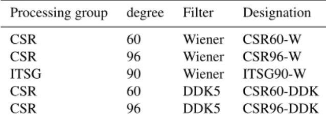
Table 1.Designations of filtered gravity field solutions.
Processing group degree Filter Designation
CSR 60 Wiener CSR60-W
CSR 96 Wiener CSR96-W
ITSG 90 Wiener ITSG90-W
CSR 60 DDK5 CSR60-DDK
CSR 96 DDK5 CSR96-DDK
its geodetic mission phase (2008–2013) are not used for the altimetry time series. Both satellites have a repeat track of approximately 10 days and the same orbital plane, which re-sults in a ground-track separation of approximately 315 km, or 2.8◦, at the Equator.
The steric component of sea level rise is determined us-ing measurement profiles of temperature and salinity from the Argo float network. Since the first deployments of Argo floats in the year 1999, the number of Argo floats has in-creased rapidly to approximately 3900 floats in the present day. Argo reached maturity around the year 2007, when at least 3000 floats were in the water (Canabes et al., 2013), which means that there is, on average, approximately 1 float per 3×3◦box. For the North Atlantic Ocean, steric sea lev-els can be analysed from 2004, because most areas are sam-pled already by Argo floats as shown in Fig. 1. In the North Atlantic Ocean, the areas around the Antilles and north of Ireland are the only problematic areas. Most floats descend to a depth around 1000–2000 m and measure temperature and salinity while travelling upward. The resurfacing time of an Argo float is approximately 10–12 days. Using the dis-tribution of temperature and salinity over depth, the steric sea level is computed.
The Earth’s time-variable gravity field is measured since 2002 by GRACE. This mission measures changes in the Earth’s gravity field by low Earth orbit satellite-to-satellite tracking. Traditionally the Earth’s gravity field is expressed in spherical harmonics. In this study, the release five monthly spherical harmonic solutions computed at the Center for Space Research (CSR) (Tapley et al., 2004), together with the ITSG-GRACE2016 solutions (Klinger et al., 2016) com-puted at the Institute for Theoretical geodesy and Satel-lite Geodesy (ITSG). The CSR solutions are computed up to degree and order 60 and 96, while the ITSG solutions are computed up to degree and order 90. All three prod-ucts are provided with full variance–covariance or normal matrices, which allows for statistically optimal filtering. In case of a proper error description, we expect that the re-sults of the CSR 60 and 96 degree solutions give compa-rable results, except in areas with large gradients in gravity. However, since the differences in variance–covariance matri-ces are small during the periods July 2003–December 2010 and February 2011–July 2013, but the orbit geometry sub-stantially varies within these periods, the provided variance–
covariance matrices are not expected to give a proper repre-sentation of the error, which leads to reduced quality filtering. Klinger et al. (2016) showed that the gravity field variability over the oceans indeed increases substantially during periods when GRACE enters repeat orbits. As a consequence, the months July–October 2004 are excluded from the analysis, when GRACE entered a near 4-day repeat orbit. The addi-tion of the ITSG soluaddi-tions enables us to compare an inde-pendent solution computed with a different approach to the standard CSR products. The non-dimensional gravity field coefficients are converted to units of equivalent water height (EWH) before filtering, to make them compatible with the other two observing systems. For comparison, we also used the publicly available Dense Decorrelation Kernel (DDK)-filtered solutions of CSR; however, no variance–covariance matrices for those solutions are publicly available. From here on, the designations listed in Table 1 are used to refer to the GRACE gravity field solutions. In the processing phase, the atmospheric and ocean de-aliasing level 1B (AOD1B) prod-uct is incorporated (Dobslaw et al., 2013), which is based on the Ocean Model for Circulation and Tides (OMCT) and the European Centre for Medium-range Weather Forecast (ECMWF) model. Monthly averages of the OMCT and the ECMWF are restored after processing to the time-varying gravity field in the form of spherical harmonics (Chambers and Willis, 2010); details of this are described in Sect. 3.3.
3 Methodology
The data described in the previous section are processed such that they are suited for establishing monthly regional sea level budgets. It implies that the equation
¯
hsla,GIA= ¯hssla+ ¯hmca,GIA (1)
is satisfied within uncertainties, whereh¯sla,GIA is the
GIA-corrected mean sea level (MSL) anomaly derived from the Jason satellites,h¯ssla the mean steric sea level anomaly
de-rived from Argo andh¯mca,GIA the mean GIA-corrected MC
anomaly in terms of EWH derived from GRACE. Note that MSL is inverse barometer-corrected and the MC anomaly from GRACE is made consistent. This section therefore de-scribes the processing strategies for the three observation types from individual measurements to an average over a specified region in the ocean including the propagation of the formal errors.
As far as altimetry is concerned, after computing individ-ual along-track sea level anomalies, two important process-ing steps are described in this section: a suitable averagprocess-ing method to come to a time series of MSL for a given area and a way to deal with geographical dependencies of the inter-mission bias between the two Jason inter-missions (Ablain et al., 2015).
July 2004
−80˚ −80˚
−70˚ −70˚
−60˚ −60˚
−50˚ −50˚
−40˚ −40˚
−30˚ −30˚
−20˚ −20˚
−10˚ −10˚
0˚ 0˚
10˚ 10˚
0˚ 0˚
10˚ 10˚
20˚ 20˚
30˚ 30˚
40˚ 40˚
50˚ 50˚
60˚ 60˚
0 10 20 30 40 50 60 70 80 90 100
July 2013
−80˚ −80˚
−70˚ −70˚
−60˚ −60˚
−50˚ −50˚
−40˚ −40˚
−30˚ −30˚
−20˚ −20˚
−10˚ −10˚
0˚ 0˚
10˚ 10˚
0˚ 0˚
10˚ 10˚
20˚ 20˚
30˚ 30˚
40˚ 40˚
50˚ 50˚
60˚ 60˚
0 10 20 30 40 50 60 70 80 90 100
Figure 1.Number of Argo floats within a 10×10◦box for grid cells where the depth is larger than 1000 m. Only floats considered in this study are used for the statistics (Sect. 3.2). The black dots indicate no floats in the 10×10◦box.
Of Seawater-2010 (TEOS-10) software is used (Pawlow-icz et al., 2012). Since the Argo measurements are non-homogeneously distributed over the ocean, the steric sea lev-els are first interpolated using an objective mapping proce-dure to a grid of 1×1◦before being averaged.
Monthly GRACE solutions of CSR and ITSG are provided with full variance–covariance and normal matrices, which allows the use of an anisotropic Wiener filter (Klees et al., 2008). Compared to other existing filters, it strongly reduces the stripes that are still present in the DDK-filtered solutions (as will be shown in Sect. 4), while not reducing the spatial resolution by applying a large Gaussian filter. A fan filter is applied after the optimal filter to reduce ringing artefacts that occur close to Greenland due to the limited number of spher-ical harmonic coefficients (degree and order 60–96). 3.1 Jason sea level
Individual sea level anomalieshslameasured with the Jason-1
and Jason-2 satellites are computed with respect to the mean sea surface (mss) DTU13 as
hsla=a−(R−1Rcorr)−mss, (2)
where a is the satellite altitude, R the Ku-band range and 1Rcorrthe applied geophysical corrections obtained from the RADS database. The satellite altitude is taken from the GDR-D orbits and the latest versions of the geophysical corrections are applied, as listed in Table 2. The 35 s smoothed dual-frequency delay is used to reduce the relatively large noise in the individual ionospheric corrections. For the wet tro-pospheric correction, we use the latest delay estimate from the radiometer, while the dry tropospheric delay is com-puted from the ECMWF pressure fields. Tidal corrections from the GOT4.10 model are applied, which are based on
Jason data instead of TOPEX data as in the GOT4.8 model (Ray, 2013). The Cartwright–Taylor–Edden solid earth tide model is applied (Cartwright and Taylor, 1971; Cartwright and Edden, 1973) and an equilibrium model for the pole tide (Wahr, 1985). For the sea state bias correction, a non-parametric model is used (Tran et al., 2012). To correct for high-frequency (<20 days) wind and pressure effects on the sea surface, a dynamic atmospheric correction is applied based on the MOG2D model (Carrère and Lyard, 2003). The dynamic atmosphere correction in RADS also includes an inverse barometer correction, which corrects for the low-frequency (>20 days) sea level anomalies caused by re-gional sea level pressure variations with respect to the time-varying global mean over the oceans. Sea level anomalies larger than 1 m are removed from further processing, as in the National Oceanic and Atmospheric Administration (NOAA) GMSL time series (Masters et al., 2012).
In GMSL time series, an intermission bias correction is applied, which is determined from the average GMSL dif-ference between Jason-1 and Jason-2 during their tandem phase, in which the satellites orbit the same plane only a minute apart (Nerem et al., 2010). However, the differences reveal a geographical dependence as shown in Fig. 2. Re-gional sea level budgets established in this study are more prone to these geographical differences than when estimat-ing global sea level budgets. This problem is partly corrected for by estimating a polynomial through the intermission dif-ferences, which only depends on latitude (Ablain et al., 2015) and is given by
1hsla,ib(λ)=c0+c1·λ+c2·λ2+c3·λ3+c4·λ4, (3)
whereλ is the latitude and 1hsla,ib(λ) is the intermission
inter-Figure 2.Geographical differences between Jason-1 and Jason-2 sea level estimates averaged over the tandem period.
Table 2.List of geophysical corrections applied in this study and for the MSLs of NOAA.
This study NOAA
Ionosphere Smoothed dual frequency Smoothed dual frequency Wet troposphere Radiometer Radiometer
Dry troposphere ECMWF ECMWF
Ocean tide GOT4.10 GOT4.8
Loading tide GOT4.10 GOT4.8
Pole tide Wahr Wahr
Solid Earth tide Cartwright–Taylor–Edden Cartwright–Taylor–Edden
Sea state bias Tran2012 CLS11
Dynamic atmosphere MOG2D MOG2D
mission differences is then computed as
hsla,c=hsla−1hsla,ib. (4)
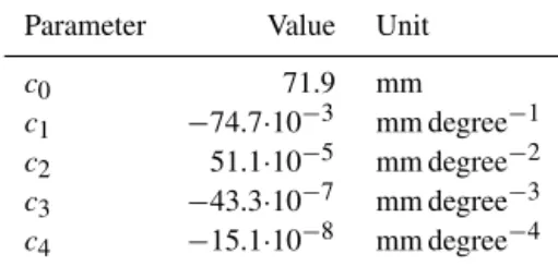
This correction is only applied to Jason-2 sea level anoma-lies. The parameters cn, with n=0,1, . . .4, depend on the
applied geophysical corrections. For the corrections given in Table 2, the values for the parameters are given in Table 3. In the middle of the North Atlantic Ocean (approximately 40◦N), the intermission difference is several millimetres less than when only including the constantc0parameter (which is slightly different if the other parameters are not estimated). This results in an approximate trend difference of several tenths of a millimetre over a period of 10 years.
Due to the limited sampling of the Argo network and the relatively large errors in the gravity field solutions it is nec-essary to integrate sea level anomalies over extended areas. Previous studies producing GMSL time series have used two different techniques (Masters et al., 2012): gridding or
lati-tude weighting based on the inclination of the orbit (Wang and Rapp, 1994; Nerem, 1995), which was simplified for a spherical Earth approximation by Tai and Wagner (2011). From here on, the latter is referred to as the Wang and Rapp method. The gridding method is problematic when using the Jason satellites, because of their large track spacing at the Equator, causing the number of individual observations per grid cell to decrease at low latitudes (Henry et al., 2014). A solution is to increase the grid cell size, but this has a disad-vantage if sea level budgets are constructed over an irregular and/or a small polygon. The Wang and Rapp method has the disadvantage that it underweights measurements at high lati-tudes (>50◦) (Scharroo, 2006), because it assumes the num-ber of measurements to reach infinity at the inclination of the satellites.
to the measurements to the number of measurementsNl in a
latitude bandlof 1◦and the area of the sea surfaceAlin the
following way: ωi(l)=
Al
Nl
. (5)
These weights are normalized: wi =
ωi
PI i=1ωi
. (6)
A MSL anomalyh¯slafor an area is computed with ¯
hsla= ˆwThˆsla,c, (7)
where wˆ is the vector of normalized weights and hˆsla,c is
the vector of sea level anomalies corrected for intermission differences.
For the error estimation, variance–covariance matrices are computed as described in Le Traon et al. (1998). Observa-tions over depths smaller than 1000 m are removed using the general bathymetric chart of the oceans (GEBCO) 1 min grid, because Argo steric sea level is referenced to this depth. This method separates the long-wavelength errors from the representativity errors due to ocean variability. White mea-surement noise is not considered here, because it becomes very small when averaged over large areas. Among the long-wavelength errors, we consider the orbit, ocean tide and in-verse barometer errors. These errors are assumed to be fully correlated between measurements within the track and un-correlated between inter-track measurements. It is noted that those correlations do not hold over large basins (>2000 km in the zonal direction) (Le Traon et al., 1998), and therefore the error is overestimated. For the other error sources, an e-folding decorrelation time of 15 days is assumed and the zero crossing of the correlation distance functiondcorris given by
(Le Traon et al., 2001): dcorr=50+250
900 λ2
avg+900
, (8)
whereλavgis the average latitude of two measurements.
Ulti-mately, this results in equations for the covariance of respec-tive measurements in different tracks and on the same track:
hǫi, ǫji =ρijσov2
hǫi, ǫji =ρijσov2 +σlw2 , (9)
whereρijis correlation computed with the decorrelation time
and distance provided above,σov2 is the ocean variability vari-ance andσlw2 is the long-wavelength variance. The values for σov andσlw are assumed to be 100 and 15 mm, where the
first number comes from typical mesoscale variability (Chel-ton et al., 2007). By putting these equations in the variance– covariance matrixCsla, the standard errorσ¯slafor the mean
sea level anomaly is computed using
¯
σsla= p
ˆ
wCslawˆT. (10)
Table 3.Values for the parameters of the intermission difference correction.
Parameter Value Unit
c0 71.9 mm
c1 −74.7·10−3 mm degree−1
c2 51.1·10−5 mm degree−2
c3 −43.3·10−7 mm degree−3
c4 −15.1·10−8 mm degree−4
Both the satellite altimetry mean sea level anomalies as well as the MC from GRACE are affected by GIA. For the corrections to GRACE and altimetry, we use the solution of Peltier et al. (2015) based on an Earth model with VM5a vis-cosity profile and ICE-6G deglaciation history. The altimet-ric measurements are corrected by subtracting the GIA geoid trend averaged over the region of interest. Errors in the GIA trends are typically assumed to be on the order of 30 % of the signal (Von Schuckmann et al., 2014).
Because the CSR gravity fields are created on a monthly basis and the altimetry measurements are averaged over a cy-cle of approximately 10 days, the altimetry measurements are low-pass filtered. A low-pass filterflpis computed by taking an inverse discrete time Fourier transform, which results in flp=
sin(2π fc(t−tm))
π(t−tm) , (11)
withfcthe cut-off frequency, which is taken as 12 cycles per
year,t is time vector of the altimetry time series andtmthe
time at the middle of a month. This filter is infinitely long, so therefore we cut it at 2 months. To obtain a better frequency response, the filter is windowed using a Hamming window wH, so that
wH=0.54−0.46 cos(
2π(t−tm−L/2)
L ), (12)
whereLis the length of the window which is 2 months. The applied filterhlpis then written in the time domain as
hlp=flp·wH. (13)
The mean of the GIA-corrected, low-pass filtered time series is subtracted, which leaves the MSL anomalyh¯sla,GIAfrom
Eq. (1).
3.2 Argo steric sea level
values measured by Argo to the absolute salinitySA(Grosso et al., 2010) as well as the ITS-90 temperatures to conserva-tive temperature2as defined in the TEOS-10 user manual (IOC, 2010). The TEOS-10 program numerically integrates the equation for the geostrophic steric sea level (IOC, 2010):
hssl= −
1 g0
P
Z
P0 ˆ
δ(SA(P′), 2(P′), P′)dP′, (14)
whereP0is the surface pressure,P is the reference pressure,
which is set to 1000 dbar (approximately 1000 m depth) and g0is a constant gravitational acceleration of 9.763 m s−2.
In the analysis, only profiles that reach at least 1000 m depth are included and have at least a measurement above 30 m depth, which is the typical depth of the mixed layer. A virtual measurement is created at 1 m depth, assuming the same salinity and potential temperature values as the highest real measurements, so that the top steric signal is not missed. Only measurements that have error flag “1” (good) or “2” (probably good) are used and the measurements are cleaned by moving a 5×5◦block to remove steric sea level estimates more than 3 rms from the mean.
To be able to average measurements monthly over a basin or a polygon, a grid is constructed by statistical interpolation of the steric sea levels at the profile locations based on the method described in Bretherton et al. (1976) and Gaillard et al. (2009). First, a background field is constructed by esti-mating a model through the 1000 closest measurements of a profile or grid cell location. This model contains a constant, a second-order 2-D longitude–latitude polynomial and six intra-annual to annual cycles (Roemmich and Gilson, 2009). The background sea surface height is taken as the model eval-uated at the grid cell (or profile) location.
Consecutively, the background field vector hˆssl,b is
sub-tracted from the sea level estimates, which results in δhˆssl= ˆhssl− ˆhssl,b, (15)
whereδhˆssl are the residuals. The ocean varianceσt2is
as-sumed to be 100 cm2(typical mesoscale variability) (Chelton et al., 2007), which is close to the average squared rms of fit of the differences of the measurements with the model. These variances are subdivided into three components to represent different correlation scales (Roemmich and Gilson, 2009) as follows:
σ12=0.77σt2 σ22=0.23σt2
σ32=0.15σt2, (16)
which are then used to construct covariance matricesCbased on those used for the Scripps fields (Roemmich and Gilson, 2009), such that
C(d)=σ12e−(140d )2+σ2 2e−
d
1111, (17)
and the measurement and representativity error matrixR:
R=diag(σ32), (18)
whered is a measure for the distance between the profilesp and the grid pointsg, such that
d=qa2dx2+dy2. (19) The parametera is one above 20◦ latitude and below this latitude thatadecays linearly to 0.25 at the Equator, in order to represent the zonal elongation of the correlation scale here (Roemmich and Gilson, 2009).
Using the covariances Cpg (between profiles and grid
points) and Cp (between profiles), the weight matrix Kis
computed as
K=Cpg(Cp+R)−1. (20)
The weight matrix is then used to compute a vector of steric sea levelshˆssl,gfor every grid point within the area:
ˆ
hssl,g=Kδhˆssl+ ˆhssl,b, (21)
for which also the variance–covariance matrixCssl,gis
com-puted, so that
Cssl,g=Cg−KCpgT, (22)
whereCgare the covariances of the background grid.
To average the steric sea level anomalies, the values are weighted by the cosine of the latitude, which results in
ωi =cos(λi). (23)
Like for altimetry, the weights are normalized: wi=
ωi
PI
i=0ωi
. (24)
Eventually these are used to compute the mean steric sea levelh¯ssland its associated errorσ¯ssl, with
¯
hssl= ˆwThˆssl,g, (25)
and
¯
σssl= q
ˆ wTC
ssl,gwˆ. (26)
Subtraction of mean from the mean steric sea level time se-ries yields the steric sea level anomaliesh¯sslaused in Eq. (1). 3.3 GRACE mass
of the signal to filter the coefficients. With the variance– covariance matricesCxandDxfor the errors and the signals,
respectively, the spherical harmonic coefficientsxˆare filtered as
ˆ
xof =(C−x1+D
−1
x )
−1C−1
x xˆ. (27)
For the filtered coefficients xˆof, a corresponding variance–
covariance matrixCx,ofis computed. This is a joint inversion
of a static background field, which is set to zero, and the time-varying coefficients, resulting in
Cx,of =(C−x1+D
−1
x )
−1. (28)
The derivation is elaborated upon in Appendix A.
The filtered grids contain ringing effects around strong signals over Greenland and the Amazon region, which can have substantial effects on the estimated trends in the ocean, which is discussed in Sect. 4. If averaged over large areas this will have hardly an effect, but on regional scales the ringing should be reduced. To obtain smoother fields, we use a fan filter (Zhang et al., 2009; Siemes et al., 2012), which is given as
ˆ
xff =sinc(
ˆ l lmax
)◦sinc( mˆ lmax
)◦ ˆxof, (29)
where the degreeˆland ordermˆ are related to the maximum degree, lmax. For a maximum degree of 60 and 96, this is
comparable to a Gaussian filter of 280 and 110 km, respec-tively (Siemes et al., 2012). SupposeFf =diag(sinc(
ˆ
l
lmax)◦
sinc(lmˆ
max)); then, the resulting covariance matrix Cx,ff is
written as
Cx,ff =FfCx,ofFf. (30)
Note that there is a fundamental difference between filtering the CSR and ITSG solutions. The CSR solutions are com-puted with respect to a static gravity field, while the ITSG solutions are computed with the respect to a static gravity field including a secular trend and an annual cycle. As a con-sequence, the CSR spherical harmonic coefficients and signal variance–covariance matrices include the annual and the sec-ular trend during Wiener and fan filtering. The ITSG gravity fields are Wiener-filtered first, then the annual cycle and the secular trend are added back and eventually the fan filter is applied.
Since the degree-1 coefficients are not measured by GRACE, we add those of Swenson et al. (2008) to the CSR solutions. For the ITSG solutions, a dedicated degree-1 solu-tion is computed using the same approach. Furthermore, we replace theC20 coefficient with satellite laser ranging
esti-mates (Cheng et al., 2013).
The intersatellite accelerations of GRACE are de-aliased for high-frequency ocean and atmosphere dynamics with the Atmospheric and Ocean De-aliasing Level-1B (AOD1B)
product. Monthly averages of the AOD1B are provided as the GAD product for both CSR and ITSG, where the mass changes over land are set to zero. To be able to combine the GRACE MC with inverse barometer-corrected altimetry, the GAD products containing the modelled oceanic and atmo-sphere mass are added back in the form of spherical harmon-ics. Because the ocean model in the AOD1B product is made mass conserving by adding/removing a thin uniform layer of water to or from the ocean, the degree zero is removed be-fore subtraction from the GAD product to compensate for the mean atmospheric mass change over the ocean, which is not measured by inverse barometer-corrected altimetry (Cham-bers and Willis, 2010).
To compute the MC at a specific grid cell, the 4π-normalized associated Legendre functionsyˆ are evaluated at its latitude–longitude location. The MC of the grid cellhmc is consecutively calculated with
hmc= ˆyTxˆff. (31)
For multiple grid cells, the vector yˆ becomes a matrix Y, such thathˆmcbecomes a vector of EWHs. This is written in
the form
ˆ
hmc=YTxˆff. (32)
It is possible to compute the grid’s variance–covariance ma-trixCmc(Swenson and Wahr, 2002) as
Cmc=YTCx,ffY. (33)
The averaging over an area is equal to that of the Argo grids. Suppose thatwˆ are the normalized latitude weights for the gridded MC; then
¯
hmc= ˆwThˆmc (34)
is the mean MC of an area and
¯
σmc= p
ˆ wTC
mcwˆ (35)
is its error.
To correct the GRACE MC for the GIA trend, we first convert the GIA spherical harmonic coefficients into EWH. The GRACE degree-2 coefficients are different than those for the altimetry, due to changes in the Earth’s rotation axis (Tamisiea, 2011). Note that GRACE only measures degrees 2 and higher, and therefore the coefficients of degree 0 and 1 are not taken into account. Eventually, the GIA spherical harmonic coefficients are converted to spatial grids, which are then averaged over the considered area, and consecutively the mean GRACE MC is corrected for the mean GIA trend.
The mean MC anomalyh¯mca,GIA used in Eq. (1) is
ob-tained by applying the GIA correction to the mean MCh¯mc
−80 −40 0 40 80 120
2004 2006 2008 2010 2012 2014
Sea level anomaly [mm]
Year
NOAA Wang and Rapp This study This study + geographical intermission bias
Figure 3.Comparison between North Atlantic mean sea level time series of NOAA (green), the Wang and Rapp method (red), our method (blue) and our method using a geographically dependent intermission bias correction and the latest geophysical corrections (light blue).
4 Comparison with existing products
In this section, a comparison is made between existing prod-ucts and the sea levels from altimetry, gravimetry and Argo floats. First, we compare the MSL time series over the North Atlantic Ocean with the existing time series provided by the NOAA Laboratory for Satellite Altimetry (Leuliette and Scharroo, 2010) and we show the effect of a latitude-dependent intermission bias. Secondly, amplitude and trend grids of steric sea level are compared to those computed from Scripps salinity and temperature grids (Roemmich and Gilson, 2009) and the Glorys reanalyses grids (Ferry et al., 2010). Thirdly, the optimal and fan-filtered gravimetry grids are compared to the DDK5-filtered gravity fields (Kusche, 2007; Kusche et al., 2009).
4.1 Total sea level
Figure 3 shows a comparison of the NOAA time series with the ones computed in this study for the North Atlantic Ocean north of 30◦N. The NOAA time series were computed by averaging over 3×1◦grid cells and then weighting them ac-cording to their latitude. The green, red and blue time series are all computed using the same geophysical corrections as given in the second column of Table 2, while the geophysi-cal correction in the first column are applied to the light blue line.
As visible from the figure, hardly any differences are ob-served between all four time series. The rms differences be-tween all time series computed in this study and NOAA are on the order of 3–4 mm, which is slightly larger than differ-ences found between the GMSL time series (Masters et al., 2012). The fact that the red and blue line resemble each other indicates that the under-weighting of high-latitude measure-ments in the Wang and Rapp method hardly has any effect on the trend. This also holds for averaging over smaller areas in the North Atlantic Ocean, where the only noticeable
differ-ence occurs when a substantial number of satellite tracks are missing due to some maintenance or orbit manoeuvres. How-ever, the time series may differ in places where strong decor-relations or strong differences in trends occur, especially in the north–south direction at high latitudes.
The application of a latitude-dependent intermission bias has a substantial effect on the trend. From the NOAA time series, a trend of 1.5 mm yr−1is found, while the time
se-ries from the Wang and Rapp method and our method pro-vide a trend of 1.8 mm yr−1. This difference can be explained by the combination of another averaging technique and geo-graphically varying trends in sea level. However, if the dif-ference in MSL is computed between 1 and Jason-2 over the North Atlantic Ocean during the tandem phase and this used as the intermission bias correction, trends of 1.3 and 1.4 mm yr−1, respectively, for the theoretical and the empirical weighting method are found. This is comparable to the trend computed by applying the geographical depen-dence of the intermission bias (the light blue line), which is 1.4 mm yr−1. To further illustrate this, Fig. 4 shows the differences in trend if a constant intermission bias is used or a latitude-dependent one is used. The mean difference of 0.4 mm yr−1is already significant, but locally the differences
in trend increase to approximately 0.8 mm yr−1. 4.2 Steric sea level
resem-Figure 4.Differences in sea level trends computed with and without a latitude-dependent intermission bias.
ble each other quite closely. However, to be able to create a variance–covariance matrix between grid cells, it was re-quired to do a 2-D interpolation of the steric sea levels in-stead of a 3-D interpolation of temperature and salinity pro-files. In order to do this, the criteria for removing profiles, as described in Sect. 3.2, is different for both methods. As a consequence of the 2-D interpolation and the differences in the removal criteria, the results differ.
In terms of the amplitudes of the annual signal, all three methods provide similar results in terms of the large-scale features. Typically, large signals are found in the Gulf Stream region and close to the Amazon Basin, while the areas around Greenland and west of Africa have small amplitudes. The Glorys grid differs from the others primarily in the Labrador Sea and northwest of Ireland. Secondly, the grid computed in this study and the Glorys grid exhibit more short-wavelength spatial variability than the Scripps grid. As long as the re-gions over which budgets are made are large enough, the methods will not differ substantially in terms of annual am-plitude.
The plots in the right column of Fig. 5 immediately re-veal a significant difference between the statistical methods and the reanalysis in terms of trend. It is not completely clear what the cause for this difference is. Since the Scripps grid
and our grid resemble each other in terms of large-scale fea-tures and are purely based onT /S data, we trust the inter-polation of Argo. The differences between those two meth-ods are again primarily the noise in the grids and the area around the Antilles, where Argo samples poorly, as discussed in Sect. 2.
4.3 Mass component
sig-(a) −80˚ −80˚ −70˚ −70˚ −60˚ −60˚ −50˚ −50˚ −40˚ −40˚ −30˚ −30˚ −20˚ −20˚ −10˚ −10˚ 0˚ 0˚ 10˚ 10˚ 0˚ 0˚ 10˚ 10˚ 20˚ 20˚ 30˚ 30˚ 40˚ 40˚ 50˚ 50˚ 60˚ 60˚
0 20 40 60 80 mm (b) −80˚ −80˚ −70˚ −70˚ −60˚ −60˚ −50˚ −50˚ −40˚ −40˚ −30˚ −30˚ −20˚ −20˚ −10˚ −10˚ 0˚ 0˚ 10˚ 10˚ 0˚ 0˚ 10˚ 10˚ 20˚ 20˚ 30˚ 30˚ 40˚ 40˚ 50˚ 50˚ 60˚ 60˚
−10 −5 0 5 10 mm yr−1
(c) −80˚ −80˚ −70˚ −70˚ −60˚ −60˚ −50˚ −50˚ −40˚ −40˚ −30˚ −30˚ −20˚ −20˚ −10˚ −10˚ 0˚ 0˚ 10˚ 10˚ 0˚ 0˚ 10˚ 10˚ 20˚ 20˚ 30˚ 30˚ 40˚ 40˚ 50˚ 50˚ 60˚ 60˚
0 20 40 60 80 mm (d) −80˚ −80˚ −70˚ −70˚ −60˚ −60˚ −50˚ −50˚ −40˚ −40˚ −30˚ −30˚ −20˚ −20˚ −10˚ −10˚ 0˚ 0˚ 10˚ 10˚ 0˚ 0˚ 10˚ 10˚ 20˚ 20˚ 30˚ 30˚ 40˚ 40˚ 50˚ 50˚ 60˚ 60˚
−10 −5 0 5 10 mm yr−1
(e) −80˚ −80˚ −70˚ −70˚ −60˚ −60˚ −50˚ −50˚ −40˚ −40˚ −30˚ −30˚ −20˚ −20˚ −10˚ −10˚ 0˚ 0˚ 10˚ 10˚ 0˚ 0˚ 10˚ 10˚ 20˚ 20˚ 30˚ 30˚ 40˚ 40˚ 50˚ 50˚ 60˚ 60˚
0 20 40 60 80 mm (f) −80˚ −80˚ −70˚ −70˚ −60˚ −60˚ −50˚ −50˚ −40˚ −40˚ −30˚ −30˚ −20˚ −20˚ −10˚ −10˚ 0˚ 0˚ 10˚ 10˚ 0˚ 0˚ 10˚ 10˚ 20˚ 20˚ 30˚ 30˚ 40˚ 40˚ 50˚ 50˚ 60˚ 60˚
−10 −5 0 5 10 mm yr−1
(a) −80˚ −80˚ −70˚ −70˚ −60˚ −60˚ −50˚ −50˚ −40˚ −40˚ −30˚ −30˚ −20˚ −20˚ −10˚ −10˚ 0˚ 0˚ 10˚ 10˚ 0˚ 0˚ 10˚ 10˚ 20˚ 20˚ 30˚ 30˚ 40˚ 40˚ 50˚ 50˚ 60˚ 60˚
0 20 40 60 80 mm (b) −80˚ −80˚ −70˚ −70˚ −60˚ −60˚ −50˚ −50˚ −40˚ −40˚ −30˚ −30˚ −20˚ −20˚ −10˚ −10˚ 0˚ 0˚ 10˚ 10˚ 0˚ 0˚ 10˚ 10˚ 20˚ 20˚ 30˚ 30˚ 40˚ 40˚ 50˚ 50˚ 60˚ 60˚
−10 −5 0 5 10 mm yr−1
(c) −80˚ −80˚ −70˚ −70˚ −60˚ −60˚ −50˚ −50˚ −40˚ −40˚ −30˚ −30˚ −20˚ −20˚ −10˚ −10˚ 0˚ 0˚ 10˚ 10˚ 0˚ 0˚ 10˚ 10˚ 20˚ 20˚ 30˚ 30˚ 40˚ 40˚ 50˚ 50˚ 60˚ 60˚
0 20 40 60 80 mm (d) −80˚ −80˚ −70˚ −70˚ −60˚ −60˚ −50˚ −50˚ −40˚ −40˚ −30˚ −30˚ −20˚ −20˚ −10˚ −10˚ 0˚ 0˚ 10˚ 10˚ 0˚ 0˚ 10˚ 10˚ 20˚ 20˚ 30˚ 30˚ 40˚ 40˚ 50˚ 50˚ 60˚ 60˚
−10 −5 0 5 10 mm yr−1
(e) −80˚ −80˚ −70˚ −70˚ −60˚ −60˚ −50˚ −50˚ −40˚ −40˚ −30˚ −30˚ −20˚ −20˚ −10˚ −10˚ 0˚ 0˚ 10˚ 10˚ 0˚ 0˚ 10˚ 10˚ 20˚ 20˚ 30˚ 30˚ 40˚ 40˚ 50˚ 50˚ 60˚ 60˚
0 20 40 60 80 mm (f) −80˚ −80˚ −70˚ −70˚ −60˚ −60˚ −50˚ −50˚ −40˚ −40˚ −30˚ −30˚ −20˚ −20˚ −10˚ −10˚ 0˚ 0˚ 10˚ 10˚ 0˚ 0˚ 10˚ 10˚ 20˚ 20˚ 30˚ 30˚ 40˚ 40˚ 50˚ 50˚ 60˚ 60˚
−10 −5 0 5 10 mm yr−1
(g) −80˚ −80˚ −70˚ −70˚ −60˚ −60˚ −50˚ −50˚ −40˚ −40˚ −30˚ −30˚ −20˚ −20˚ −10˚ −10˚ 0˚ 0˚ 10˚ 10˚ 0˚ 0˚ 10˚ 10˚ 20˚ 20˚ 30˚ 30˚ 40˚ 40˚ 50˚ 50˚ 60˚ 60˚
0 20 40 60 80 mm (h) −80˚ −80˚ −70˚ −70˚ −60˚ −60˚ −50˚ −50˚ −40˚ −40˚ −30˚ −30˚ −20˚ −20˚ −10˚ −10˚ 0˚ 0˚ 10˚ 10˚ 0˚ 0˚ 10˚ 10˚ 20˚ 20˚ 30˚ 30˚ 40˚ 40˚ 50˚ 50˚ 60˚ 60˚
−10 −5 0 5 10 mm yr−1
nal is lost in the CSR60-W and CSR96-W solutions. Thirdly, Tamisiea et al. (2010) estimated a slight increase in MC am-plitudes using fingerprint methods based on forward models of water mass redistribution around the Sahel and Amazon of 10–15 mm. In the Wiener-filtered CSR grids, larger plitudes are also visible in these regions; however, their am-plitude of 30–60 mm is far too large and is probably the result of hydrological leakage. This leakage is slightly reduced in CSR96-W compared to those of the CSR60-W.
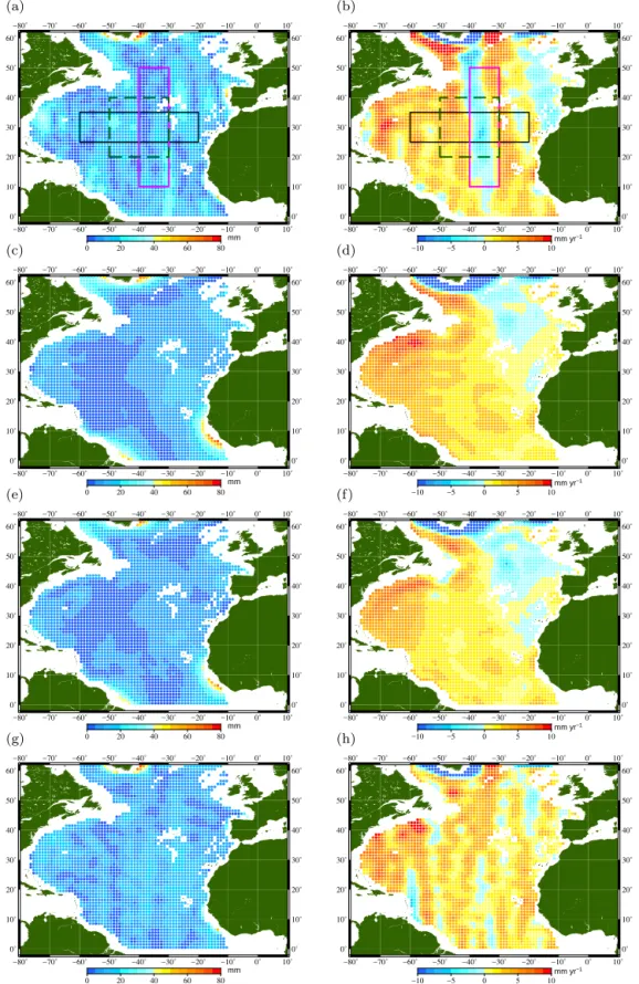
To determine how this effects sub-basin-scale MC time series, it is first required to determine the minimum area over which the measurements have to be integrated. GRACE gravity fields have a resolution of typically 250–300 km half wavelength (Siemes et al., 2012). For small ocean signals af-ter applying filaf-tering procedures, we expect the resolution to be closer to 400–500 km. Argo has approximately one to two floats per 3×3◦box, so its resolution is in the same range as that of GRACE. Jason-1 and Jason-2 have an inter-track spacing of 315 km at the Equator, which decreases substan-tially towards 60◦N. Considering all systems, this theoreti-cally makes it possible to create budgets over grid cells of approximately 500×500 km; however, due to the limited length of the time series, the error bars on the trends be-come much larger than the signals. The size of the polygons is therefore chosen based on the criterion that the error on the trends does not exceed 1 mm yr−1.
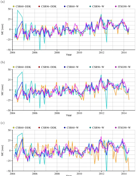
To illustrate the effects of different filters and residual striping on sub-basin-scale budgets, Fig. 7 shows time se-ries of mass averaged over the polygons shown in Fig. 6. All three polygons have approximately the same size, but have different orientations. The location is chosen in the middle of the Atlantic to avoid effects of hydrological leakage. Except for the months surrounding the near 4-day repeat period in 2004, where the variance–covariance matrices of CSR prob-ably do not properly described the noise of the gravity fields, the time series resemble each other best for the zonally ori-ented polygon. In the zonal polygon, the noise in CSR96-W is substantially larger than the other results. Furthermore, it becomes clear that the CSR96-DDK solutions do not con-tain a substantial signal above degree 60, because the red and yellow lines are on top of each other, while CSR60-W and CSR96-W are substantially different.
The month-to-month noise of CSR60-W and CSR96-W time series is comparable for all three polygons. The CSR60-DDK and CSR96-CSR60-DDK time series become much noisier for the meridionally oriented polygon, where month-to-month jumps of 10–20 mm occur. In addition, the DDK time se-ries exhibit a substantially different trend in the meridional polygon than the other time series, because the orientation of the polygon is aligned with the residual stripes (Fig. 6). So, in terms of trend and noise, the DDK time series strongly depends on the orientation of the polygon. Even though the ITSG90-W trend and amplitude grids suffer from striping, they do not become significantly noisier for the meridionally oriented polygon.
5 Results and discussion
The first objective of this section is to reveal patterns of sea level amplitudes and trends in the North Atlantic Ocean and how these resemble for the two different methods: altime-try and the combined method of Argo and GRACE, here-after referred to as Argo+GRACE. Secondly, this section discusses the closure of sea level budgets over polygons of approximately 1/10 of the North Atlantic Ocean in terms of trend, annual amplitude and residual variability. It is shown for which regions the budget is closed and possible causes for non-closure are discussed. Thirdly, we focus on the best choice of GRACE filter solutions for the MC.
5.1 North Atlantic sea level patterns
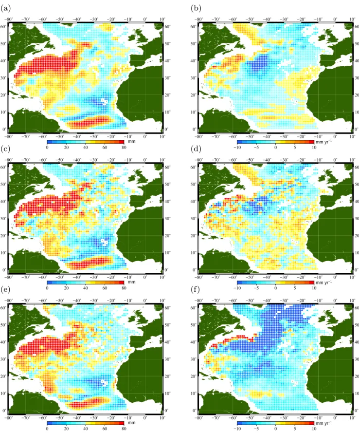
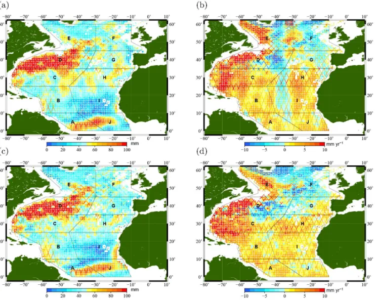
In Fig. 8, grids of trends and amplitudes computed from Argo+GRACE are overlaid with Jason-derived trends and amplitudes at the ground tracks. In areas where the ground tracks of altimetry are barely visible, there is a good resem-blance between Argo+GRACE and altimetry.
The grids and ground tracks shown in the left column show that large annual signals are present in the Gulf Stream region and in a tongue stretching from the Amazon to the Sahel. A region without any substantial annual signal is lo-cated just west of Africa, which is clearly visible in both the Argo+GRACE grid and altimetry. Both methods reveal these large-scale oceanographic features in amplitude, but there are also quite some differences. East of the Antilles, altimetric measurement show an annual amplitude of more than 60 mm, whereas Argo+GRACE estimates are in the range of 40– 50 mm, depending on the choice of GRACE filter. Note that in this area, there are barely any Argo floats (Fig. 1), which might lead to interpolation problems. A second difference is observed in the Wiener-filtered grid (bottom left) at the Ama-zon and Sahel regions. This is exactly at the areas where the Wiener-filtered MC grids of Fig. 6 exhibit probable hydro-logical leakage.
The trends from altimetry in the right column of Fig. 8 show a distinct pattern, where positive trends are found south of 35◦N and negative trends north of it, with the exception of the North American coastline. Large trends along the North American coast are also found by tide gauge studies (Sal-lenger at al., 2012), where they attribute this to a weakening Atlantic meridional overturning circulation (AMOC). The Argo+CSR96-W solution resembles the trend patterns de-rived from altimetry measurement better, while the residual stripes in the CSR96-DDK solution are clearly visible. Note that a significantly larger altimetric trend is visible west of the Mediterranean. Possible causes will be discussed below. 5.2 Sub-basin-scale budgets
(a)
−50 −25 0 25 50
2004 2006 2008 2010 2012 2014
MC [mm]
Year
CSR60−DDK CSR96−DDK CSR60−W CSR96−W ITSG90−W
(b)
−50 −25 0 25 50
2004 2006 2008 2010 2012 2014
MC [mm]
Year
CSR60−DDK CSR96−DDK CSR60−W CSR96−W ITSG90−W
(c)
−50 −25 0 25 50
2004 2006 2008 2010 2012 2014
MC [mm]
Year
CSR60−DDK CSR96−DDK CSR60−W CSR96−W ITSG90−W
Figure 7.Sub-basin-scale time series of the MC using various filters for three polygons with different orientation: zonal(a), square(b)and meridional(c). Red and yellow represent the CSR60-DDK and the CSR96-DDK solutions. The blue and light blue time series represent, respectively, the CSR60-W and the CSR96-W solutions. In purple are the time series of the ITSG90-W solution.
through the major oceanographic features in the latitudinal direction, like the salt water tongue in front of the Mediter-ranean and the Gulf Stream, as shown in Fig. 8. Any ob-servations within 200 km from the coast are excluded using a grid provided by Goddard Space Flight Center (GSFC). Just as in Sect. 4.3, the size of the regions is chosen such that the error on the trends does not exceed 1 mm yr−1. First, we will discuss three representative examples of time series.
Figure 8.Amplitudes of the annual signal (left) and trends (right) computed of the sum of the components (Argo+GRACE) overlayed with those computed from the total sea level measured with altimetry. For the two top figures, the CSR96-DDK(a, b)solutions are used and for the bottom two, the CSR96-W(c, d)solution is used.
5.2.1 Time series
Budgets for three representative regions, using the Wiener-filtered MC solutions, are shown in Fig. 9. The time series for the rest of the regions can be found in the Supplement. The left plots confirm that the main driver for annual fluctuations in sea level is the steric sea level, but that the trend is strongly influenced by a mass component. On the right side, we see that the sum of the components and the total sea level agree to within the error bars, but some problems arise in the Gulf Stream area (region D), probably caused by sharp gradients in sea level. The sea levels in polygons D and I also contain some interannual signals, which is especially pronounced be-tween 2010 and 2012. The left column shows that the inter-annual variability is primarily a steric signal. Note that the larger size of the error bars in regions B and I is due to the decrease in altimetry track density closer to the Equator and
the elongation of the correlation radius for the interpolation of Argo floats.
5.2.2 Trends
Region B
−100 −50 0 50 100
2004 2006 2008 2010 2012 2014 2004 2006 2008 2010 2012 2014
Sea level [mm]
Year Year
Total Steric Mass Total Mass+Steric
Region D
−100 −50 0 50 100
2004 2006 2008 2010 2012 2014 2004 2006 2008 2010 2012 2014
Sea level [mm]
Year Year
Total Steric Mass Total Mass+Steric
Region I
−100 −50 0 50 100
2004 2006 2008 2010 2012 2014 2004 2006 2008 2010 2012 2014
Sea level [mm]
Year Year
Total Steric Mass Total Mass+Steric
Figure 9.Time series of sea level components for regions B, D and I. Left: total sea level from altimetry in red, steric sea level in green and the ITSG90-W mass in blue. Right: total sea level from altimetry in red and the sum of steric sea level and mass in blue. In yellow and light blue: their 95 % confidence interval.
Table 4.Trends of total sea level (mm yr−1) and their standard deviations from altimetry (Jason) and the sum of steric and mass from Argo (A.) and GRACE (CSR, ITSG) for different filter solutions. NA is the trend for the complete North Atlantic Ocean between 0 and 65◦N. A 0.4 mm yr−1 drift error is taken into account for altimetry based on the comparisons with tide gauges (Mitchum, 1998, 2000).
Jason CSR96+A. CSR96+A. CSR60+A. ITSG90+A. GIA GIA
DDK5 Wiener Wiener Wiener ASLa EWHb
A 2.6±0.5 1.8 2.4±0.9 2.7±0.9 2.3±0.9 −0.3 −2.2 B 2.8±0.5 3.1 3.0±0.7 3.7±0.7 3.1±0.7 −0.5 −3.4 C 3.2±0.4 4.2 4.4±0.5 4.8±0.5 4.5±0.5 −0.6 −5.1 D 1.0±0.4 1.5 1.9±0.5 3.1±0.5 2.3±0.4 −0.6 −6.0 E 0.5±0.4 2.2 0.3±0.5 0.0±0.5 2.2±0.4 −0.5 −7.1 F −2.4±0.4 −2.0 −3.4±0.5 −3.0±0.5 −1.8±0.4 −0.5 −4.6 G 0.7±0.5 −0.8 −0.2±0.6 0.0±0.6 0.4±0.6 −0.5 −3.6 H 4.7±0.4 1.4 2.5±0.6 2.7±0.6 3.3±0.6 −0.5 −3.5 I 2.3±0.4 1.4 2.1±0.6 2.5±0.6 2.5±0.6 −0.5 −2.8 J 2.4±0.4 1.7 1.3±0.7 1.3±0.7 1.6±0.6 −0.3 −2.0 NA 1.8±0.4 1.8 1.5±0.3 1.8±0.3 2.2±0.2 −0.5 −4.1
Table 5.Amplitudes (mm) of the annual signal from total sea level from altimetry and the sum of steric and mass from Argo and GRACE for different filter solutions.
Jason CSR96+A. CSR96+A. CSR60+A. ITSG90+A. A. only
DDK5 Wiener Wiener Wiener
A 42.3±1.3 36.0 26.8±3.4 28.2±3.4 36.3±3.1 32.2±3.1 B 34.2±0.9 27.5 27.8±2.7 29.6±2.7 30.5±2.5 30.2±2.4 C 54.0±0.7 52.6 49.3±2.1 48.5±2.1 52.9±1.9 47.1±1.9 D 82.1±0.6 85.0 84.3±2.0 82.8±1.9 88.3±1.7 82.6±1.7 E 48.0±0.5 43.2 40.2±1.9 38.5±1.8 42.8±1.5 39.3±1.4 F 45.8±0.6 40.4 37.6±2.0 39.6±1.9 41.2±1.6 35.1±1.6 G 45.1±0.9 44.5 37.7±2.2 39.9±2.1 43.2±2.0 38.4±1.9 H 49.9±0.8 48.8 45.1±2.3 46.5±2.3 48.1±2.1 39.6±2.1 I 18.7±0.8 19.0 16.0±2.3 17.8±2.2 19.1±2.0 11.9±2.0 J 40.3±1.2 40.8 46.1±2.5 49.0±2.4 42.9±2.2 33.9±2.1 NA 44.6±0.3 42.6 39.5±1.1 40.0±1.0 43.3±0.8 37.7±0.8
for the different MC solutions. It is important to note that es-pecially region F suffers from some ringing artefacts before the fan filter is applied and that the far northeast is not very well covered by Argo floats. The trends of CSR96-DDK in region G are a bit further off than the other solutions, proba-bly resulting from the striping, as visible in Fig. 6.
In the northwest of the Atlantic, the choice of gravity field filter either substantially influences the estimated trends (D and E), or they are just outside of 2 standard deviations (C) for one or more solutions. Using the CSR96-W solution, the budget is closed within 2 standard deviations for all three polygons, whereas the other solutions do not close the bud-get. For region C, the results of the all filters resemble one another quite well, but some are just outside of 2 standard deviations from altimetry. For region D, the CSR60-W re-sults are far off, but the other rere-sults are close again. In this region, sharp gradients occur not only in the MC with the presence of a neighbouring continental shelf but also in the steric component. This might lead to leakage of the continen-tal shelf mass signal or problematic interpolation of the Argo steric sea levels. In addition, for both of the aforementioned regions, the GIA correction on the MC is relatively large. Adding a GIA correction error of 10–20 %, which is smaller than discussed in Sect. 3.3, to the mass trends would close the budget in these regions for all the solutions, except for the CSR60-W solution in region D. In region E, a clear split is visible between the Wiener-filtered CSR solutions, which close the budget, and the other two solutions, which do not close the budget. The difference in results could be caused by the filter not being able to handle the large gradients (Klees et al., 2008) in the MC within this region (Fig. 8). However, if we would again add only a 10–20 % GIA correction error, it would suffice to close the budget for all filters.
Ultimately, only the budget in region H cannot be closed with any of the solutions and there is no strong GIA signal present, which could be responsible for a large bias. In addi-tion, the sea level in this polygon does not exhibit any strong
gradients and the number of Argo floats is substantial. This excludes interpolation or filtering problems. Therefore, we argue that this can be explained by a deep-steric effect that could be related to variations in the export of saline water from the Mediterranean (Ivanovic et al., 2014), which is not captured by Argo.
In conclusion, it is possible to close the sea level budget within two standard deviations for 9 out of 10 regions using CSR96-W. If a 10–20 % GIA correction error is taken into account, the budget for 9 out of 10 polygons is also closed for CSR96-DDK and ITSG90-W. This also suggests that the commonly assumed GIA correction error of 20–30 % (Von Schuckmann et al., 2014) is probably overestimated. 5.2.3 Annual signal
We indicated that the seasonal cycles are primarily caused by steric variations in sea level (Fig. 9). By comparing the first column with the last column in Table 5, it becomes clear that in most cases an additional mass signal is required to close the budget in terms of annual amplitude. The discrepancy be-tween Argo and altimetry for the whole North Atlantic Ocean reveals that, on average, in-phase mass signals with an am-plitude of approximately 7 mm are required to close the bud-gets, which is in line with the modelled results of Tamisiea et al. (2010). They modelled, using fingerprints, amplitudes of the MC ranging from 3 to 12 mm, and phases (not shown here) between days 210 and 330, which is in phase with the steric signal.
Region B
−100 −50 0 50 100
2004 2006 2008 2010 2012 2014 2004 2006 2008 2010 2012 2014
Sea level [mm]
Year Year
Steric Mass Total Mass+Steric
Region D
−100 −50 0 50 100
2004 2006 2008 2010 2012 2014 2004 2006 2008 2010 2012 2014
Sea level [mm]
Year Year
Steric Mass Total Mass+Steric
Region I
−100 −50 0 50 100
2004 2006 2008 2010 2012 2014 2004 2006 2008 2010 2012 2014
Sea level [mm]
Year Year
Steric Mass Total Mass+Steric
Figure 10.Time series of sea level components for polygons B, D and I after removing the trends and the annual and semiannual signals. Left: ITSG90-W mass in blue and steric sea level in green. Right: total sea level from altimetry in red and the sum of steric sea level and mass in blue.
H and I) the amplitude budget closes within 2 standard devi-ations using these solutions.
Even though no error bars are computed for the CSR96-DDK, it is clear that the results are far better in terms of budget closure. The results are comparable to ITSG90-W, which closes 7 out of 10 budgets within 2 standard devi-ations. CSR DDK5+Argo underestimates the amplitude in region B, while ITSG90-W+Argo overestimates the ampli-tude with respect to altimetry in region D. In region B, the es-timate of ITSG90-W+Argo is relatively small, and in region D, the CSR96-DDK+Argo also relatively large. Note that the number of Argo floats in region B is often small (Fig. 1) and that large gradients in the steric sea level in region D could cause interpolation problems for steric sea level. Sec-ondly, in both northern polygons E and F, both combinations of Argo+GRACE underestimate the amplitude compared to altimetry. Why this underestimation occurs is not completely clear. A likely culprit is the gravity field filtering, but yearly deep convection events in these regions (Vå ge et al., 2009), which transport surface water to depths below 1000 m, and
the limited number of Argo floats, could also be contributing factors.
Table 6.Fraction of explained variance,R2, of altimetry total sea level by Argo+GRACE steric and mass for different gravity field filter solutions after removing the semiannual and annual signals and the trend.
CSR96+A. CSR96+A. CSR60+A. ITSG90+A.
DDK5 Wiener Wiener Wiener
A 0.32 0.07 0.33 0.38
B 0.02 −0.46 0.09 0.24
C 0.37 0.14 0.38 0.40
D 0.31 0.16 0.36 0.34
E 0.14 −0.19 0.29 0.44
F 0.09 −0.17 0.45 0.52
G 0.13 −0.05 0.29 0.34
H −0.12 −0.49 0.21 0.27
I 0.34 0.14 0.50 0.49
J 0.39 0.17 0.45 0.53
NA −0.05 −1.21 −0.06 −0.01
5.2.4 Residual variability
Time series for the same regions as in Fig. 9 are shown in Fig. 10, but their trend, semiannual and annual signals have been reduced to show the residual variability. For the rest of the regions, plots of the residuals are given in the Sup-plement. In contrast to the time series for the whole North Atlantic Ocean (not shown), the sub-basin-scale time series show significant interannual variability. Region D, located at the east coast of the United States, shows a jump of 60– 70 mm within 3 months at the end of 2009. This jump co-incides with a shift in the Gulf Stream described by Pérez-Hernández and Joyce (2014) as the largest in the decade, which they related to the North Atlantic Oscillation. As il-lustrated in the left column, the shift in the Gulf Stream is primarily of steric nature; however, small deviations in the mass signal are also present. It is remarkable that at the same time on the other side of the Atlantic (region I, bottom fig-ures), an increase in sea level is observed by both altime-try and Argo. This suggest a link between the latitude of the Gulf Stream and sea level temperatures in the east of the At-lantic. In region B, we also observe a small interannual ef-fect by altimetry and Argo. However, the amplitude of the signal is larger for altimetry than is captured by Argo, which suggests either some interpolation issues in an area without many Argo floats or a deep-steric effect.
Using any of the filtered CSR or ITSG solutions, it is pos-sible to detect the interannual variability described, probably because most of the signal is of steric origin. However, for the interannual signals that are less pronounced, or for high-frequency behaviour of sea level, there are some differences between the MC solutions. Table 6 shows the fraction of vari-ance of the residual signal of altimetry (trend, semiannual and annual cycles removed) explained by Argo+GRACE.
The third column indicates that Argo in combination with CSR96-W does not explain much of the residual variance,
but mostly introduces additional noise, which causes the neg-ative values. Using the DDK5-filtered MC, the explained variance increases, but the best performance is obtained with the CSR60-W and especially the ITSG90-W gravity fields. The last column shows that after reducing the trend, and the semiannual and annual signals, between 24 and 53 % of the residual signal can be explained by the combination of Argo and ITSG90-W. It is remarkable that for the whole North Atlantic Ocean (last row), no variance is explained by the Argo+GRACE, primarily due to the absence of a clear interannual signal. Note that the value−1.21 for the CSR96-W gravity fields indicates that variance increases af-ter its subtraction from altimetry, which indicates that the Argo+GRACE time series is substantially noisier than the altimetry time series.
6 Conclusions
For the first time, it is shown that sea level budgets can be closed on a sub-basin scale. With the current length of the time series, it is possible to establish budgets over ar-eas of approximately 1/10 of the North Atlantic Ocean. To obtain error bars on the annual amplitudes, trends and time series, errors for altimetry and Argo profiles are propa-gated from existing correlation functions, while for GRACE full variance–covariance matrices are used. For altimetry, a latitude-dependent intermission bias is applied and it is shown that this leads to trend differences ranging up to 0.8 mm yr−1if the period from 2004–2014 is considered.
error is added. The results of the CSR96-DDK filter, how-ever, strongly depend on the orientation of averaging area due to residual meridional striping. The strong resemblance be-tween trends also indicates that the errors on the GIA model are probably smaller than the commonly assumed 20–30 %. Furthermore, a large difference in trend between altimetry and Argo+GRACE is observed in front of the Mediterranean Sea where only a small GIA correction is applied. We believe that this originates from steric effects below the considered 1000 m, where saline water enters the Atlantic Ocean from the Strait of Gibraltar and dives to large depths. Further re-search is needed to confirm this hypothesis.
The CSR60-W and CSR96-W solutions appear to underes-timate the amplitude of the annual signal substantially. They also suffer from what appears to be leakage around the Ama-zon and Sahel, regions with a substantial annual hydrological cycle. Using the CSR96-DDK gravity fields and the ITSG90-W solutions, the sum of the steric and mass components be-comes significantly closer to that of altimetry, with closure in 7 out of 10 regions. However, it must be noted that the altimetry signals tend to be slightly larger. This is likely due to partial destruction of the signal by filtering of the gravity fields or limited Argo coverage or, in some regions, deep-steric signals.
By removing the semiannual and annual signals and trends, interannual variability can be detected. Since most of the interannual variability in the North Atlantic Ocean is con-tained in the steric component, the type of filter on the gravity fields is not really important. However, if we look at differ-ences on a month-to-month basis, high-frequency variations or small interannual fluctuations in mass, it is best to use the CSR60-W the ITSG90-W solutions, because the fraction of explained variance of the altimetric sea level time series by the sum of the components using these solutions is largest. Using the ITSG90-W solution, 24–53 % of the variability in the altimetry-derived sea level time series is explained. The CSR96-W solution only introduces noise and explains virtu-ally no residual variability of the altimetry time series. Espe-cially in the 4-day repeat orbits in 2004 and even the months around them, the Wiener-filtered solutions do not give proper estimates of the MC, which partly contributes to a lower ex-plained variance.
Appendix A
The Wiener filter is, in principle, a joint inversion between the spherical harmonic coefficients of the background field
ˆ
xb and those of the time-varying gravity field xˆ. Suppose
thatCxis the error variance–covariance matrix ofxˆ andDx
the signal variance–covariance matrix; then the filtered coef-ficientsxˆf are expressed as
ˆ
xf =(C−x1+Dx−1)−1C−x1xˆ+(C−x1+D−x1)−1D−x1xˆb. (A1)
Assuming the spherical harmonic coefficients of the back-ground field are zero, this equation reduces to Eq. (27). Its filtered variance–covariance matrixCx,f is computed using
Cx,f =
(C−x1+D−x1)−1C−x1Cx((C−x1+D
−1
x )
−1C−1
x )T
+(C−x1+Dx−1)−1D−x1Dx((C−x1+D−x1)−1D−x1)T. (A2)
Since the matrices(C−x1+Cx−1)−1andC−x1are symmetric, it is possible to simply change the order underneath the trans-pose sign and leave
Cx,f =
(C−x1+Dx−1)−1C−x1CxC−x1(C−x1+D−x1)−1
+(C−x1+D−x1)−1D−x1DxD−x1(C
−1
x +D
−1
x )
−1, (A3)
which is further simplified by using the identityC−x1Cx=I
to
Cx,f =(C−x1+D
−1
x )
−1C−1
x (C
−1
x +D
−1
x )
−1
+(C−x1+D−x1)−1Dx−1(C−x1+D−x1)−1. (A4) Finally, this equation is rewritten, such that
Cx,f =(C−x1+D
−1
x )
−1(C−1
x +D
−1
x )(C
−1
x +D
−1
x )
−1, (A5)
Appendix B
List of abbreviations
AMOC Atlantic meridional overturning circulation ANS Anisotropic non-symmetric
AOD Atmosphere and ocean de-aliasing CSR Center for Space Research DDK Dense Decorrelation Kernel
ECCO Estimating the circulation & climate of the ocean ECMWF European Centre for Medium-range Weather Forecasts EWH Equivalent water height
GEBCO General bathymetric chart of the oceans GIA Glacial isostatic adjustment
GMSL Global mean sea level
GRACE Gravity Recovery And Climate Experiment GSFC Goddard Space Flight Center
ITSG Institute of Theoretical geodesy and Space Geodesy OBP Ocean bottom pressure
OMCT Ocean Model for Circulation and Tides
MC Mass component
MSL Mean sea level
NOAA National Oceanic and Atmospheric Administration RADS Radar Altimetry Database System
rms Root mean square