Impact of combining GRACE and GOCE gravity data on ocean circulation estimates

(1)

OSD

8, 1535–1573, 2011

GRACE/GOCE data and ocean circulation

estimates

T. Janji´c et al.

Title Page

Abstract Introduction

Conclusions References

Tables Figures

◭ ◮

Back Close

Full Screen / Esc

Printer-friendly Version Interactive Discussion

Discussion

P

a

per

|

Dis

cussion

P

a

per

|

Discussion

P

a

per

|

Discussio

n

P

a

per

Ocean Sci. Discuss., 8, 1535–1573, 2011 www.ocean-sci-discuss.net/8/1535/2011/ doi:10.5194/osd-8-1535-2011

Ocean Science Discussions

This discussion paper is/has been under review for the journal Ocean Science (OS). Please refer to the corresponding final paper in OS if available.

Impact of combining GRACE and GOCE

gravity data on ocean circulation

estimates

T. Janji ´c1, J. Schr ¨oter1, R. Savcenko2, W. Bosch2, A. Albertella3, R. Rummel3,

and O. Klatt1

1

Alfred Wegener Institute for Polar and Marine Research, Bussestrasse 24, 27570 Bremerhaven, Germany

2

Deutsches Geod ¨atisches Forschungsinstitut, Munich, Germany

3

Institute for Astronomical and Physical Geodesy, TU Munich, Munich, Germany

Received: 22 May 2011 – Accepted: 14 June 2011 – Published: 27 June 2011

Correspondence to: T. Janji´c ([email protected])

(2)

OSD

8, 1535–1573, 2011

estimates

T. Janji´c et al.

Title Page

Tables Figures

◭ ◮

Back Close

Full Screen / Esc

Discussion

P

a

per

|

Dis

cussion

P

a

per

|

Discussion

P

a

per

|

Discussio

n

P

a

per

|

Abstract

In this work we examine the impact of assimilation of multi-mission-altimeter data and the GRACE/GOCE gravity fields into the finite element ocean model (FEOM), with the focus on the Southern Ocean circulation. In order to do so, we use the geode-tic approach for obtaining the dynamical ocean topography (DOT), that combines the 5

multi-mission-altimeter data and the GRACE/GOCE gravity fields, and requires that both fields be spectrally consistent. The spectral consistency is achieved by filtering of the sea surface height and the geoid using profile approach. Combining the GRACE and GOCE data, a considerably shorter filter length resolving more DOT details can be used. In order to specify the spectrally consistent geodetic DOT we applied the 10

Jekeli-Wahr filter corresponding to 241 km, 121 km, 97 km and 81 km halfwidths for the GRACE/GOCE based gravity field model GOCO01S and to the sea surface. More re-alistic features of the ocean assimilation were obtained in the Weddel gyre area due to increased resolution of the data fields, particularly for temperature field at the 800 m depth compared to Argo data.

15

1 Introduction

One of the central topics in oceanography is reliable estimation of ocean circulation. Many authors demonstrated that the satellite altimetry is suitable for estimation of ocean circulation variability (Schr ¨oter et al., 1993; Fu and Chelton, 2001; Fukumori, 2001; Le Traon and Morrow, 2001). Attempts to assimilate variance of DOT in an eddy 20

resolving model were reported by K ¨ohl and Willebrand (2002). They applied the 4DVAR method to infer gradients of statistical moments. In the same year Staneva et al. (2002) assimilated only variability of DOT referenced to an unknown (or grossly uncertain) mean. Both studies demonstrate the need of an appropriate mean sea surface as ref-erence. Indeed Staneva et al. (2002) find an even small data misfit for variability when 25

(3)

OSD

8, 1535–1573, 2011

estimates

T. Janji´c et al.

Title Page

Tables Figures

◭ ◮

Back Close

Full Screen / Esc

Discussion

P

a

per

|

Dis

cussion

P

a

per

|

Discussion

P

a

per

|

Discussio

n

P

a

per

the importance of non linear processes in the ocean circulation, mainly advection. Therefore, to correctly estimate the mean ocean state, the assimilation of the

abso-lute dynamical topography appears to be necessary. This is a difficult task because the

ocean general circulation models commonly show systematic deviation from the mea-sured mean dynamic topography. This systematic deviation can be caused by a variety 5

of reasons including poor knowledge of surface forcing, inadequate parametrizations of subgrid processes and missing details of the bottom topography used in the model. Further, global ocean circulation models usually lack a proper representation of

high-latitude processes due to a limited model domain or insufficient resolution. On the other

side,the bottom waters occupying the major ocean basins are originating mainly from 10

Antarctic (Antarctic Bottom Water). Here, the Weddell Sea is an important source of the Antartic bottom water (Carmack, 1977; Orsi et al., 1999; Fahrbach et al., 1995, 2001; Convey et al., 2009), and thus it is a key region for the global thermohaline circulation. The ability of models together with data assimilation to better represent properties in this area are therefore crucial for ocean circulation.

15

The measured mean DOT can be constructed from geodetic data using an altimetric mean sea surface (from more than 17 yr of radar altimetry), and an accurate geoid. The DOT can also be constructed by combining in-situ oceanographic data (temperature and salinity of seawater, direct measurements of current velocity, etc). Yet another way of measured mean DOT generation is by combining the geodetic estimate (altimetry 20

and geoid) with the traditional oceanographic estimate (Niiler et al., 2003). The detailed picture of the mean ocean circulation from data only is obtained by combining the geodetic estimates of DOT with fine scale ocean observations. However, in order to be able to predict changes in ocean circulation, and to have more accurate estimates of not so well observed fields, the assimilation of DOT in the ocean model is required. 25

(4)

OSD

8, 1535–1573, 2011

estimates

T. Janji´c et al.

Title Page

Tables Figures

◭ ◮

Back Close

Full Screen / Esc

Discussion

P

a

per

|

Dis

cussion

P

a

per

|

Discussion

P

a

per

|

Discussio

n

P

a

per

|

by a separate estimate of the mean DOT from the ocean data or unconstrained ocean model.

In contrast to the usual practice of treating the mean DOT and its temporal variation

separately (Penduffet al., 2002; K ¨ohl et al., 2007; Stammer et al., 2007), in our study,

the mean DOT and its variability are not separated. Instead, time series of 10 day 5

”absolute” DOTs are generated using the satellite altimetry and our knowledge of the geoid as given by the GOCO1S model. Such a 10 day geodetic DOT time series is then assimilated into the ocean model for one year.

A major advantage of satellite observations is their global coverage and continuity in time. This is especially important, for example, for studies of the Southern Ocean. 10

There, observations using conventional techniques are sparse and had been limited to CTD measurements along hydrographic sections till Argo program started in 1999 (Fahrbach, 1999; Fahrbach and Naggar, 2001; Fahrbach et al., 2003; Fahrbach and

de Baar, 2010). Unfortunately, the radar altimetry is also not su_fficiently reliable for

those regions where the sea-ice coverage exceeds a certain percentage during the 15

entire year, or near-coastal zones. Furthermore, the extent of the ice-covered ocean area changes with the seasonal cycle, thereby averting the radar altimetry from deliv-ering complete and representative measurements over time.

The geoid from GRACE and altimetry were previously used to estimate geodetic ocean topography which was then assimilated into a numerical model in order to pro-20

duce a modified ocean circulation field (Skachko et al., 2008; Janji´c et al., 2011b). Having higher spatial resolution, the new GOCE data allow for an increase in the spec-tral content of the geodetic DOT data. The goal of this paper is to demonstrate and examine the impact of the increased spectral content of the DOT data on ocean fields, especially for the Southern Ocean. We will show that by assimilating globally DOT 25

(5)

OSD

8, 1535–1573, 2011

estimates

T. Janji´c et al.

Title Page

Tables Figures

◭ ◮

Back Close

Full Screen / Esc

Discussion

P

a

per

|

Dis

cussion

P

a

per

|

Discussion

P

a

per

|

Discussio

n

P

a

per

2 Ocean model

The ocean model used to perform this study is the Finite-Element Ocean circulation Model (FEOM) (Danilov et al., 2004; Wang et al., 2008). The model is configured

on a global, almost regular triangular mesh with spatial resolution of 1.5◦_{, and with 24}

unevenly spaced levels in the vertical. The ocean model solves the standard set of 5

hydrostatic ocean dynamics primitive equations. It uses a finite-element flux corrected transport algorithm for tracer advection (L ¨ohner et al., 1987).

The model is forced at the surface with momentum fluxes derived from the ERS scat-terometer wind stresses complemented by TAO derived stresses (Menkes et al., 1998). The vertical mixing is parameterized by Pakanowsky-Philander scheme (Pakanowski 10

and Philander, 1981). The thermodynamic forcing is replaced by restoring of surface temperature and salinity to monthly mean surface climatology of WOA01 (Stephens et al., 2002). The model is initialized by mean climatological temperature and salinity of Gouretski and Koltermann (2004).

The FEOM ocean model has been tested in several previous studies. In a recent 15

study, Sidorenko et al. (2011) compared the FEOM model to other ocean models par-ticipating in the experiment under the normalized year forcing of Coordinated Ocean-ice Reference Experiments. It was shown that the ocean state simulated by FEOM is in most cases within the spread of other models. The FEOM model was also compared to the independent data and used for data assimilation studies with real observations in 20

the work of (Skachko et al., 2008; Rollenhagen et al., 2009; Janji´c et al., 2011a,b). Fur-ther, Timmermann et al. (2009) examined the properties of the model with its standard setup, and compared its transport estimates in the Southern Ocean with those from observations. Especially hydrographic properties were simulated fairly accurately, but more research needs to be done in this context on the role of eddies, the freshwater 25

(6)

OSD

8, 1535–1573, 2011

estimates

T. Janji´c et al.

Title Page

Tables Figures

◭ ◮

Back Close

Full Screen / Esc

Discussion

P

a

per

|

Dis

cussion

P

a

per

|

Discussion

P

a

per

|

Discussio

n

P

a

per

|

3 Geodetic dynamical ocean topography

As already pointed out, the DOT can be constructed from geodetic data using an alti-metric sea surface and an accurate geoid. This apparently simple concept has to be

realized with care as the sea surface and the geoid are defined in a completely different

way: While the geoid is expressed spectrally by a spherical harmonic series, the sea 5

surface is in general provided in terms of gridded products. Therefore the mutual spec-tral consistency of these two surfaces must be ensured to avoid that unknown omission error is introduced in the DOT (Schr ¨oter et al., 2002; Losch and Schr ¨oter, 2004; Bing-ham et al., 2008). Further, it is recognized that the gridded sea surface itself is already a derived product, generated by resampling the sea surface heights originally observed 10

along the ground tracks of satellite altimetry. In this section a dedicated procedure for obtaining a time series with 10 day snapshots of DOT is explained and properties of obtained data set are discussed.

The geodetic dynamic ocean topography is defined as the difference between sea

surface heightshand geoid heightsN,

15

DOT=h₋N. (1)

First, it has to be emphasized that the two quantities to be subtracted should be

inde-pendent of each other. This implies that the geoid heightsN must be computed from

gravity field models estimated without any surface gravity which is over ocean area ob-tained from altimetry itself. Satellite-only gravity fields, derived exclusively from GRACE 20

or GOCE data satisfy this condition and avoid the risk that geoid heights are corrupted by altimetry. Thus, for this study geoid heights were computed from the ITG-Grace03s (Mayer-G ¨urr, 2007) and GOCO01S (Pail et al., 2010) gravity field models. Both

quanti-tieshandN are usually computed w.r.t. an ellipsoid of revolution. Naturally, the same

ellipsoid has to be applied. In addition, the permanent tidal deformation which is due 25

to the attraction of Sun and Moon has to be treated in the same way for both, the sea

surface and the geoid. The sea surface heights hwere computed from the

(7)

OSD

8, 1535–1573, 2011

estimates

T. Janji´c et al.

Title Page

Tables Figures

◭ ◮

Back Close

Full Screen / Esc

Discussion

P

a

per

|

Dis

cussion

P

a

per

|

Discussion

P

a

per

|

Discussio

n

P

a

per

(on its interleaved ground track). The altimetric mission, data source and repeat cycle

of each mission used for computing DOT are listed in Table 1. The di_fferent sampling

characteristics of these missions ensure the best possible spatial coverage through

the entirety of ground tracks. However, in order to apply data from different missions

a dedicated pre-processing is necessary. The altimeter data were homogenized by 5

applying the best known mission specific corrections. For the computation of altimetric sea surface heights the standard corrections provided with the used altimeter products were applied with the modifications listed in Appendix A. Moreover, common geophys-ical models have been used for correcting ocean tides and the reaction of sea level to atmospheric pressure. Subsequently relative radial error components have been esti-10

mated by means of a multi-mission crossover analysis (Dettmering and Bosch, 2010). After correcting these radial errors the altimeter data of all missions can be expected to be as consistent as possible.

The di_fferences of Eq. (1) are then directly performed with the sea surface heights

observed on the altimeter ground tracks. This method further on called profile approach 15

has several advantages. First, it avoids any initial gridding which always implies an

un-desirable smoothing that is difficult to control. Second, the original sea surface heights

observed along the ground tracks can be used with their high sampling rate. Finally, the approach treats individual profiles and consequently results in estimates of instan-taneous DOT profiles. It is then straightforward to use these DOT profiles in order to 20

generate any temporal mean representing the DOT for a specific period of time. In this paper instantaneous multi-mission DOT profiles are used to generate a time series of ten day DOT snapshots.

The difficulty to realize the profile approach is to ensure the consistent filtering of h

andN. Let 2-D[ ] be a two-dimensional filter operator, taking into account the spectral

25

properties of the geoid. A Gauss-type Jekeli-Wahr filter (Jekeli, 1981) is used here as this filter has neither side lobes in the spectral domain nor in the spatial domain. Instead of Eq. (1) the DOT should be derived by applying the 2-D filter operation

(8)

OSD

8, 1535–1573, 2011

estimates

T. Janji´c et al.

Title Page

Tables Figures

◭ ◮

Back Close

Full Screen / Esc

Discussion

P

a

per

|

Dis

cussion

P

a

per

|

Discussion

P

a

per

|

Discussio

n

P

a

per

|

whereNSATdenotes the geoid heights from the satellite only gravity field. As his not

a two dimensional quantity, but available only along track profiles, a one-dimensional

filtering 1-D[h] can be applied only. In order to account for the systematic differences

between one- and two-dimensional filtering, the identity

2-D[h]=1-D[h]+2-D[h]−1-D[h]

5

≈1-D[h]+2-D[NHR]−1-D[NHR], (3)

is used and approximated by applying the last two filter operations to an ultra-high

resolution geoid, denoted by NHR, derived from the EGM2008 (Pavlis et al., 2008),

expanded in spherical harmonics up to degree and order 2190. Combining Eqs. (2) and (3) and re-ordering the filter operations gives

10

DOT=1-D[h₋NHR]+δPG (4)

whereδPG₌2-D[NHR]−2-D[NSAT]=2-D[NHR−NSAT] is the pre-geoid correction which

can be computed in advance. Equation (4) indicates that the instantaneous DOT

pro-files can be estimated by a one-dimensional filter operation applied to the difference

between sea surface height and geoid height from EGM2008 performed for the along 15

track sequence of observation points, plus the correctionδPG evaluated at the same

points.

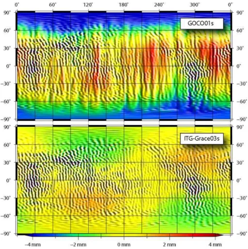
The magnitude of the pre-geoid correction is small and remains below a few mil-limetres. This is illustrated by the two panels of Fig. 1 showing for a filter length of

241 km the geographical pattern ofδPGcomputed for ITG-Grace03S (lower panel) and

20

GOCO01S (upper panel). For ITG-Grace03S the δPG values are even smaller than

for GOCO01S. This is due to the fact that ITG-Grace03S has been used to construct

the low degree part of EGM2008 (Pavlis et al., 2008). TheδPG values for GOCO01S

exhibit some systematic differences. As GOCO01S is expected to provide a much

bet-ter spatial resolution, filbet-ter operations with smaller filbet-ter length of 121 and 97 km were 25

applied to GOCO01S only. As can be seen in Fig. 2 the magnitude ofδPG is inversely

(9)

OSD

8, 1535–1573, 2011

estimates

T. Janji´c et al.

Title Page

Tables Figures

◭ ◮

Back Close

Full Screen / Esc

Discussion

P

a

per

|

Dis

cussion

P

a

per

|

Discussion

P

a

per

|

Discussio

n

P

a

per

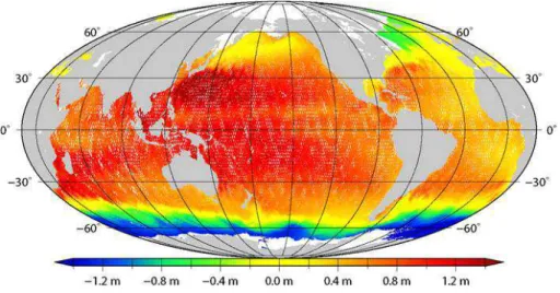
The results of the profile approach described thus far are instantaneous DOT pro-files. Gridded DOT values can be obtained from the DOT profiles by the application of gridding procedures for any arbitrary chosen time period. The Fig. 3 shows the snap-shot of the multi-mission DOT computed for ten days around 25 April 2004 using the filter length of 121 km. The sequence of ten day DOTs used for the assimilation are 5

generated by linear interpolation onto finite element grid of model using weighted mean of values from profiles lying in the cell near grid nodes. The weights were obtained by means of linear distance depending weighting. All measurements lying within ten day period were used. Therefore, the exact time in which measurement was made was not taken into account. Figure 3 shows the lack of data (white region) in the Southern 10

Ocean where the ice covered area drifts zonally with the seasonal cycle so that the sig-nificant part of the surface appears to be ice-covered at least for some time during the year. In particular, the Weddell Sea is without any data coverage. Further data gaps are seen in ten day estimates of DOT. These result from the interpolation of the

altime-try profiles to the model grid, with an area of influence of 2◦

×2◦. This interpolation is

15

kept as local as possible to avoid any additional filtering of the data. The described procedure produces for every 10 days maps of DOT. The mean over 10 day maps was calculated in order to investigate the information content of these data sets.

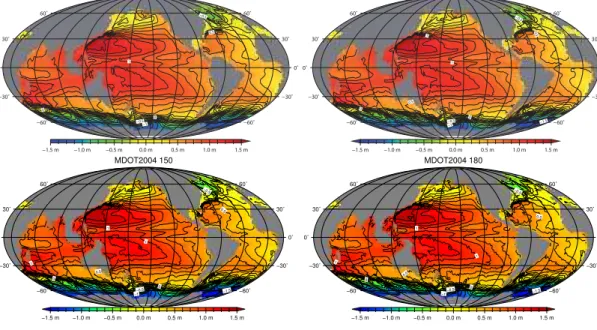
In Fig. 4 mean over one year DOTs obtained using profile approach are shown for Jekeli-Wahr filter with half width of 241 km (upper left), 121 km (upper right), 97 km 20

(lower left) and 81 km (lower right). The result of GOCO1s model filtered up to degree half width of 241 km was compared to the results using ITG-Grace03s. As can been

seen in Fig. 5 where the di_fference between two mean fields is shown, these are almost

identical. Small differences that do not exceed 0.5 cm can be still noted (see Fig. 5).

In Fig. 5 also the differences between geodetic DOTs filtered with different half width

25

are plotted. Filtering to the smaller half widths allow much more details to remain in

both altimetric and gravity field data. In particular, the main differences between the

(10)

OSD

8, 1535–1573, 2011

estimates

T. Janji´c et al.

Title Page

Tables Figures

◭ ◮

Back Close

Full Screen / Esc

Discussion

P

a

per

|

Dis

cussion

P

a

per

|

Discussion

P

a

per

|

Discussio

n

P

a

per

|

parallel positive and negative bands that appear in the regions of strong ocean currents such as ACC, Gulf Stream, the Kuroshio Current and its extension, and the equatorial

currents. These are visible if one compares the difference between results obtained

by filtering to half width of 241 km and 121 km (see Fig. 5 upper right) and to much

lesser extent in the di_fference between 121 km and 97 km filtered results (lower left).

5

The difference between the mean DOTs obtained as result of the filtering between

97 km (lower left) and 81 km on the other side seem to be dominated by the noise. Further improvements are expected for these half widths once six months of GOCE data instead of only two is used.

Therefore, the effect of filtering is to smear out the gradient resulting in weaker and

10

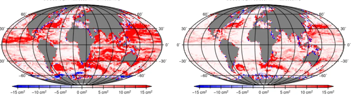
less well defined estimates of the ocean currents. The use of only satellite data starting with half width of 121 km show fine space scales that were previously poorly resolved with half width of 241 km. However, also the time variability of the data set are attenu-ated as a result of spatial filtering. Increase in resolution of the DOT is accompanying the increase in the variability. In Fig. 6 increase in variance is shown by the change of 15

the filter length from 241 km to 121 km to 97 km. The figure shows the increase of the signal variance of sequences of ten day DOT grids by decrease of the filter lengths. The most significant changes occur in the change of the filter length from 241 km to 121 km. The further reduction of the filter length leads to significant increase of the variances in the areas of significant variability of sea surface e.g. Gulf and Kuroshio 20

streams. The apparent dilution of variance in polar and coastal areas can be explain by the better performance of the filter with the small filter length near the critical areas e.g. coast or sea ice boundaries.

4 Assimilation of DOT data

Details of the data assimilation algorithm are described in Janji´c et al. (2011b,a) for 25

(11)

OSD

8, 1535–1573, 2011

estimates

T. Janji´c et al.

Title Page

Tables Figures

◭ ◮

Back Close

Full Screen / Esc

Discussion

P

a

per

|

Dis

cussion

P

a

per

|

Discussion

P

a

per

|

Discussio

n

P

a

per

order to take into account higher resolution data. Further we describe the filtering prop-erties of the assimilation scheme depending on the data that is being assimilated and

compare differences in the results of assimilation.

Four simulations were performed for the period between January 2004 and Decem-ber 2004. These simulations were free model run, i.e. a model integration within the 5

chosen time period without data assimilation and three simulations with assimilation of data filtered up to 241 km, 121 km and 97 km. For assimilation simulations, time vary-ing DOT data are assimilated every 10 days. The data assimilation scheme corrects all the ocean fields, although only geodetic DOT is assimilated. A diagonal observation error covariance matrix is used with 5 cm STD for data filtered up to 241 km, 121 km 10

and 7 cm STD for data filtered up to 97 km.

We use the domain localized singular evolutive interpolated Kalman filter (SEIK) al-gorithm (Pham et al., 1998; Pham, 2001; Nerger et al., 2006) as implemented within the parallel data assimilation framework (PDAF, Nerger et al., 2005). We update the full model state, consisting of temperature, salinity, SSH, and velocity fields. The SEIK 15

algorithm is used together with the method of weighting of observations proposed by Hunt et al. (2007). In Janji´c et al. (2011a) it was shown that a) the optimal influence

region is a circle with a radius of 900 km (cutofflength) for observations that are filtered

to half width 241 km and b) that optimal covariance for localization of ensemble Kalman filter algorithm approximates well a Gaussian with length scale of 246 km. For the data 20

filtered up to 121 km, experiments were performed using the same specification, as

well as a localization function with length scale of 123 km (450 km cutoff). For these

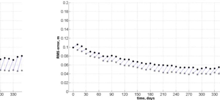
two experiments Fig. 7 shows the 10 day time evolution of the RMS error of the SSH for analysis and forecast compared to the data assimilated over the entire ocean. Further

experiments with different length scale of localization function confirmed that length

25

scale of 123 km (450 km cutoff) is optimal for observations that are filtered to half width

(12)

OSD

8, 1535–1573, 2011

estimates

T. Janji´c et al.

Title Page

Tables Figures

◭ ◮

Back Close

Full Screen / Esc

Discussion

P

a

per

|

Dis

cussion

P

a

per

|

Discussion

P

a

per

|

Discussio

n

P

a

per

|

to the geodetic DOT) to 4 cm for analysis and 5 cm for the prediction if proper cuttoff

length, depending on the data that is assimilated, is used. Accordingly, the length scale

of localization function was chosen to have the 360 km cutofffor observations that are

filtered to half width 97 km.

As an example, mean DOTs obtained as result of assimilation of data filtered up to 5

degree 121 km are presented in Fig. 8. The mean DOT obtained by averaging 10 day outputs from the simulations can be subtracted from a corresponding mean geodetic

DOT. The differences between the observations and the assimilation results of data

filtered up to degree 121 km are presented in Fig. 9 for the mean DOTs obtained both from the analysis and from the forecast. Similarly as in case of assimilation of data 10

filtered to other degrees, di_fferences between mean forecasted field and the data have

the maximum amplitudes in the open ocean in the Southern Ocean east of South

America and in between 70◦_{E and 120}◦_{E, as well as at 140}◦_{W. These locations are}

characterized by strong eddy activity. Di_fferences are also larger along the west Pacific

coast, in the Labrador Sea area, as well close to the Indonesian region. 15

In order to investigate the ability of the data assimilation scheme to incorporate the

higher resolution data into the model, the di_fference between the mean analysis

ob-tained as a result of assimilation of different resolution of data is considered. Figure 10

shows the difference between mean fields for assimilation of data with the half width of

241 and 121 km as well as the di_fference in results for assimilation of data with 121 km

20

and 97 km. Similar pattern and magnitudes are shown in Fig. 5 for data only fields. The increase in resolution from the half width of 241 to 121 km modifies the fields with

the di_fferences that can exceed 10 cm, while the changes from the half width of 121 to

97 km are smaller.

Figure 11 shows the details of the mean DOT obtained as the result of analysis and 25

(13)

OSD

8, 1535–1573, 2011

estimates

T. Janji´c et al.

Title Page

Tables Figures

◭ ◮

Back Close

Full Screen / Esc

Discussion

P

a

per

|

Dis

cussion

P

a

per

|

Discussion

P

a

per

|

Discussio

n

P

a

per

in South Atlantic where the turning of the Subantartic front now coincides with the estimates of location of this front by Orsi et al. (1995) (full black lines in Figs. 10 and 11). However, some features that are seen in the mean analysis are not seen in the mean forecast anymore, indicating the inconsistency between the data and ability of the model to predict them.

5

Figure 12 shows the magnitude of the velocity at 50 m depth from mean of forecast for the three assimilation results. In this figure also the magnitude of the geostrophic velocities computed from 6 months of GOCE data and altimetry (Albertella et al., 2011) filtered up to half width of 97 km is shown. Increase in resolution of the data primarily

effects the magnitudes of velocities. These are increasing for forecasted velocities at

10

50 m with the increase in resolution of DOT data. Stronger velocities are observed in the areas where ACC fronts are quite close to one another or in case of meandering of the currents. Forecasted velocities at 50 m depth agree very well with the geostrophic velocities as calculated from data only filtered up to half width of 97 km, with slightly lower magnitudes.

15

Finally it is interesting to compare the assimilation results in the area which is only partially observed by altimetry, namely Weddell Sea. For this comparison we use the independent Argo data set to show the impact of assimilation of global DOT.

5 Validation of results

5.1 Data set used for validation

20

For the validation of the results of the assimilation of DOT filtered to different halfwidths,

we use the Argo data set (http://www.argo.ucsd.edu, http://argo.jcommops.org). Since 1999 more than 200 Argo floats were deployed in the vicinity of the Weddell Gyre. These floats drift with the ocean currents at typically 800 m depth, collecting vertical profiles of temperature and salinity between 2000 m depth and the sea surface every 25

(14)

OSD

8, 1535–1573, 2011

estimates

T. Janji´c et al.

Title Page

Tables Figures

◭ ◮

Back Close

Full Screen / Esc

Discussion

P

a

per

|

Dis

cussion

P

a

per

|

Discussion

P

a

per

|

Discussio

n

P

a

per

|

standards. The additional delayed mode quality control for salinity was performed as described in (Owens and Wong, 2009), comparing float data to a high quality reference CTD data (climatology). These comparisons are made on deep isotherms and assume that the temperature sensor of the float is stable and that salinity on deep isotherms is

steady and uniform. The accuracy of the float data is better than 0.01◦_{C in}

tempera-5

ture and 0.01 in salinity. The floats are modified with ice sensing algorithm, and have RAFOS tracking allowing them to operate during winter (Klatt et al., 2007).

A cycling period of 10 days allows using subsurface displacements as a direct and absolute measurement of the oceans’ velocity at the parking depth (800 m mostly). For the comparison in this study velocity components are calculated using the first 10

Argos fix from the present cycle and the last Argos fix from the previous cycle and dividing each underwater displacement by its corresponding exact duration

(Nunez-Riboni et al., 2005). The velocities were averaged into 1.5◦ _{longitude by 1}◦ _latitude

bins. A simple low-pass filter (calculating the average of a bin and all of its eight immediate neighbors) was applied in each bin.

15

In Fig. 13 locations of the Argo floats used for this calculation are plotted. These floats are used in our study for validation only. In Fig. 13 (right) the Weddell gyre flow and in-situ temperature at 800 m are shown as estimated from Argo data. At

about 30◦_{E, both temperature and flow field show clearly the southward spreading of}

waters influenced by the ACC, resulting in an intrusion of warm water masses with 20

temperatures of about 1◦_{C into Antarctic waters. From about 60}◦_{S southward, these}

waters spread to the west as part of the southern branch of the Weddell Gyre. Their subsequent transformation into deep and bottom water feeds the global thermohaline circulation. Additional southward float displacements are just about visible to the east of

Conrad Rise at about 50◦_{E. Possibly, warmer waters from the north are entrained here}

25

into the Weddell Gyre as well, which would be consistent with (Park and Gamb ´eroni,

1995), who place the boundary of the Weddell Gyre as far east as 60◦_{E near the}

(15)

OSD

8, 1535–1573, 2011

estimates

T. Janji´c et al.

Title Page

Tables Figures

◭ ◮

Back Close

Full Screen / Esc

Discussion

P

a

per

|

Dis

cussion

P

a

per

|

Discussion

P

a

per

|

Discussio

n

P

a

per

at (58◦_{S, 10}◦_{E), this observation supports the double cell structure of the Weddell}

Gyre as suggested by (Beckmann et al., 1999). Again the Subantartic, Polar and ACC fronts as estimated from historical station data (Orsi et al., 1995) are superimposed on the Fig. 13. It is interesting to note very good agreement between ACC front line as estimated by Orsi et al. (1995) and the Argo composite results.

5

5.2 Results of global assimilation of DOT

In Fig. 14 the temperature at 800 m depth is plotted for four simulations. Model only re-sults show generally warmer water than observed. East of prime meridian temperature

below 0.5◦_{C are not obtained.}

RMS values calculated for the area presented in Fig. 14 with model only results 10

compared to Argo as well as for the three assimilation simulations are shown in Table 2.

For the area north of 60◦_{S, the RMS values are smaller for temperature, and higher}

for velocities. Use of data assimilation decreased the RMS errors for temperature and slightly for velocities once the data filtered to half width of 241 km are used. Further, improvements can be noted when data with higher spectral resolution is assimilated. 15

The RMS values for assimilation of data filtered to 97 km are 0.35◦_{C for temperature}

and 3.4, 2.4 cms−1_{for velocity, north of 60}◦_{S values are 0.22}◦_{C, 4 and 2.8 cm s}−1_.

Most striking difference between model only and assimilation results is however a

spatial structure of temperature at 800 m depth. Area in between ACC and Polar front is represented better with use of the data assimilation and with use of higher resolution 20

data. Warmer water is entrained between the front lines as result of assimilation in

the area between 25◦_{W and 50}◦_{W, for example. Similarly with higher resolution data,}

area 25◦_{E to 50}◦_{E and north of 54}◦_{S shows better agreement to the Argo data. Minima}

at 58◦_{S at 10}◦_{E in the Argo data is seen in the assimilation of global DOT results,}

however more east than observed. Temperature in the area between 25◦_{W to 25}◦_E

25

are now significantly closer to observed by ARGO. Also, water masses characterized

by lower than observed temperature west of 30◦_{W are closer to observed values with}

(16)

OSD

8, 1535–1573, 2011

estimates

T. Janji´c et al.

Title Page

Tables Figures

◭ ◮

Back Close

Full Screen / Esc

Discussion

P

a

per

|

Dis

cussion

P

a

per

|

Discussion

P

a

per

|

Discussio

n

P

a

per

|

at 800 m level. Also temperature field south of 66◦_{S still is warmer then observed by}

Argo data.

6 Conclusions

Geodetic DOT with much finer space scales, that were previously poorly resolved, is obtained by combining GRACE and GOCE gravity field data. These data fields are 5

constructed for every 10 days. Mean obtained by averaging 10 day geodetic estimates of DOT shows fine space scale structures, that are particularly visible in the areas of strong currents. Both the mean filed and variability of this data set are attenuated as a result of spatial filtering. Such a global geodetic data set was assimilated in the finite element ocean model. Results of assimilation into the global finite element ocean 10

model, shows similar increase in the resolution of DOT obtained as seen in the data.

In this work we investigated the impact of assimilation of global DOT data with diff

er-ent resolution. We showed that by assimilating globally DOT data, the model simulation can be further improved. This is shown also for the Southern Ocean that is not well

observed south of 60◦_{S and that plays a crucial role for properly representing ocean}

15

circulation. Comparison of the results with independent Argo data set shows positive impact of assimilation not only for DOT fields, and close to the surface, but also in tem-perature field at 800 m depth. Once the temtem-perature and salinity data are assimilated in the model, further improvements in results are expected.

Appendix A 20

Mission specific corrections

(17)

OSD

8, 1535–1573, 2011

estimates

T. Janji´c et al.

Title Page

Tables Figures

◭ ◮

Back Close

Full Screen / Esc

Discussion

P

a

per

|

Dis

cussion

P

a

per

|

Discussion

P

a

per

|

Discussio

n

P

a

per

models for the mean ocean tide models, geoid heights, and reaction of sea level to atmospheric pressure were used. For the computation of altimetric sea surface heights, the standard corrections provided with the used altimeter products (see Table 1) were applied with the following modifications:

1. for GFO the ionospheric corrections were computed from GIM ionospheric model 5

scaled with the IRI model (Iijima et al., 1999);

2. all corrections described in Schrama et al. (2000) were applied to the ERS-1/2 data sets;

3. the orbit data of ERS-1/2 was replaced by DEOS precise orbits (Scharroo and Visser, 1998);

10

4. the GDR ENVISAT orbits were replaced by ESA orbits of GDR-C standards;

5. for Jason1 the radiometer wet troposphere correction are replaced using replace-ment product provided by Jet Propulsion Laboratory (JPL) (S. Desai, personal communication, 2009);

6. for the sea state bias of TOPEX, the model of Chambers et al. (2003) was used; 15

7. the orbits of TOPEX and Jason-1 missions were replaced by Lemoine et al. (2010);

8. for Jason-1, TOPEX/Poseidon and ENVISAT, the dual frequency ionospheric cor-rections were smoothed by means of median filter with the filter length of 20 s;

9. the TOPEX microwave radiometer are replaced using replacement product 20

(S. Desai, personal communication, 2003);

(18)

OSD

8, 1535–1573, 2011

estimates

T. Janji´c et al.

Title Page

Tables Figures

◭ ◮

Back Close

Full Screen / Esc

Discussion

P

a

per

|

Dis

cussion

P

a

per

|

Discussion

P

a

per

|

Discussio

n

P

a

per

|

11. for all altimeter systems the ocean tide corrections were computed using the EOT10a (Mayer-G ¨urr et al., 2011) tide model;

The second step was the multi-mission-cross-calibration. The radial error compo-nent and relative mission specific biases were corrected by means of multi-mission-crossover analysis (Dettmering and Bosch, 2010).

5

Acknowledgements. This work has been funded under DFG Priority Research Programme

SPP 1257 “Mass Transport and Mass Distribution in the Earth System”.

References

Albertella, A., Savcenko, R., Janji´c, T., Rummel, R., Bosch, W., and Schroeter, J.: First experi-ments with high resolution dynamical topography computation from GOCE, Geophys. J. Int., 10

submitted, 2011. 1547, 1571

Beckmann, A., Hellmer, H., and Timmermann, R.: A numerical model of the Weddell Sea:large-scale circulation and water mass distribution, J. Geophys. Res., 104, 23374–23391, 1999. 1549

Bingham, R. J., Haines, K., and Hughes, C. W.: Calculating the Ocean’s Mean Dynamic Topog-15

raphy from a Mean Sea Surface and a Geoid., J. Atmos. Ocean. Technol., 25, 1808–1822, 2008. 1540

Carmack, E.: Water charachteristics of the Southern Ocean south of the Polar Front, in: Angel, M. (ed.), A voyage of discovery–George Deacob 70th Anniversary Volume, 15–41, Pergamon Press, 1977. 1537

20

Chambers, D. P., Hayes, S. A., Ries, J. C., and Urban, T. J.: New TOPEX sea state bias models

and their effect on global mean sea level, J. Geophys Res., 108, 3305, 2003. 1551

Convey, P., Bindschadler, R., di Prisco, G., Fahrbach, E., Gutt, J., Hodgson, D., Mayewski, P., Summerhayes, C., and Turner, J.: Antarctic Climate Change and the Environment, Antarct. Sci., 21, 541–563, doi:10.1017/S0954102009990642, 2009. 1537

25

Danilov, S., Kivman, G., and Schr ¨oter, J.: A finite-element ocean model: principles and evalua-tion, Ocean Model., 6, 125–150, 2004. 1539

(19)

OSD

8, 1535–1573, 2011

estimates

T. Janji´c et al.

Title Page

Tables Figures

◭ ◮

Back Close

Full Screen / Esc

Discussion

P

a

per

|

Dis

cussion

P

a

per

|

Discussion

P

a

per

|

Discussio

n

P

a

per

Fahrbach, E.: Die Expedition ANTARKTIS XV/4 des Forschungsschiffes POLARSTERN 1998 :

[28. Mrz 1998 - 23. Mai 1998, Punta Arenas - Kapstadt]=The expedition ANTARKTIS XV/4

of the research vessel POLARSTERN in 1998, Berichte zur Polar- und Meeresforschung=

Reports on polar and marine research 314, Alfred Wegener Institute for Polar and Marine Research, 1999. 1538

5

Fahrbach, E. and de Baar, H.: The expedition of the research vessel POLARSTERN to the Antarctic in 2008 (ANT-XXIV/3) / ed. by Eberhard Fahrbach and Hein de Baar, Berichte zur

Polar- und Meeresforschung=Reports on polar and marine research 606, Alfred Wegener

Institute for Polar and Marine Research, 2010. 1538

Fahrbach, E. and Naggar, S. E.: Die Expeditionen ANTARKTIS XVI/1-2 des Forschungsschiffes

10

POLARSTERN 1998/1999=The expeditions ANTARKTIS XVI/1-2 of the research vessel

POLARSTERN in 1998/1999, Berichte zur Polar- und Meeresforschung=Reports on polar

and marine research 380, Alfred Wegener Institute for Polar and Marine Research, 2001. 1538

Fahrbach, E., Rohardt, G., Scheele, N., Schr ¨oder, M., Strass, V., and Wisotzki, A.: Formation 15

and discharge of deep and bottom water in the northwestern Weddell Sea, J. Mar. Res., 53/4, 515–538, 1995. 1537

Fahrbach, E., Harms, S., Rohardt, G., Schr ¨oder, M., and Woodgate, R.: Flow of bottom water in the northwestern Weddell Sea, J. Geophys. Res., 106, 2761–2778, 2001. 1537

Fahrbach, E., Fuetterer, D. K., and Naggar, S. E. D. E.: Die Expedition ANTARKTIS XVIII/3-20

4 des Forschungsschiffes POLARSTERN 2000/2001 sowie die Aktivitaeten an Land und

bei der Neumayer-Station = The expedition ANTARKTIS XVIII/3-4 of the research vessel

POLARSTERN in 2000/2001 including operations on land and at the Neumayer Station,

Berichte zur Polar- und Meeresforschung = Reports on polar and marine research 445,

Alfred Wegener Institute for Polar and Marine Research, 2003. 1538 25

Fahrbach, E., Hoppema, M., Rohardt, G., Boebel, O., Klatt, O., and Wisotzki, A.: Warming of deep and abyssal water masses along the Greenwich meridian on decadal time scales: The

Weddell gyre as a heat bu_ffer, Deep.-Sea Res. Pt. II, in press, 2011. 1572

Fu, L. and Chelton, D.: Large-scale ocean circulation, in Sattelite Altimetry and Earth Sciences, Int. Geophys.Ser., 69, edited by: Fu, L. L. and Cazenave, A., 133–169, Academic, San Diego, 30

Calif., 2001. 1536

(20)

OSD

8, 1535–1573, 2011

estimates

T. Janji´c et al.

Title Page

Tables Figures

◭ ◮

Back Close

Full Screen / Esc

Discussion

P

a

per

|

Dis

cussion

P

a

per

|

Discussion

P

a

per

|

Discussio

n

P

a

per

|

2001. 1536

Gouretski, V. V. and Koltermann, K. P.: WOCE Global Hydrographic Climatology, Bundesamt

f ¨ur Seeschifffahrt und Hydrographie, Hamburg und Rostock, Germany, 2004. 1539

Hunt, B. R., Kostelich, E. J., and Szunyogh, I.: Efficient Data Assimilation for Spatiotemporal

Chaos: A local Ensemble Transform Kalman filter., Physica D, 230, 112–126, 2007. 1545 5

Iijima, B. A., Harris, I. L., Ho, C. M., Lindqwister, U. J., Mannucci, A. J., Pi, X., Reyes, M. J., Sparks, L. C., and Wilson, B. D.: Automated daily process for global ionospheric total elec-tron content maps and satellite ocean ionospheric calibration based on Global Positioning System, J. Atmos. Sol.-Terr. Phy., 61, 1205–1218, 1999. 1551

Janji´c, T., Nerger, L., Albertella, A., Schroeter, J., and Skachko, S.: On domain localization 10

in ensemble based Kalman filter algorithms., Special collection -Intercomparisons of 4D-Variational Assimilation and the Ensemble Kalman Filter. Early online edition, Mon. Weather Rev., doi: 10.1175/2011MWR3552.1, 2011a. 1539, 1544, 1545

Janji´c, T., Schr ¨oter, J., Albertella, A., Bosch, W., Rummel, R., Savcenko, R., Schwabe, J., and Scheinert, M.: Assimilation of geodetic dynamic ocean topography using ensemble based 15

Kalman filter, J. of Geodynam., nn, nn, 2011b. 1538, 1539, 1544

Jekeli, C.: Alternative methods to smooth the earth’s gravity field., in: Dept. Geod. Sci. and Surv., Ohio State University, Columbus., rep. 327, 1981. 1541

Klatt, O., Boebel, O., and Fahrbach, E.: A Profiling Float’s Sense of Ice, J. Atmos. Ocean Technol., 24, 1301–1308, 2007. 1548, 1572

20

K ¨ohl, A. and Willebrand, J.: An adjoint method for the assimilation of statistical characteristics into eddy-resolving ocean models, Tellus, 54, 406–425, 2002. 1536

K ¨ohl, A., Stammer, D., and Cornuelle, B.: Interannual to Decadal Changes in the ECCO Global Synthesis, J. Phys. Oceanogr., 37, 313–337, 2007. 1538

Le Traon, P. and Morrow, R.: Ocean Currents and Eddies, in Sattelite Altimetry and Earth 25

Sciences, Int. Geophys.Ser, 69, edited by: Fu, L. L. and Cazenave, A., 171–215, Academic, San Diego, Calif., 2001. 1536

Lemoine, F., Zelensky, N., D.S.Chinn, Pavlis, D., Rowlands, D., Beckley, B., Luthcke, S., Willis, P., Ziebart, M., Sibthorpe, A., Boy, J., and Luceri, V.: Towards development of a consistent orbit series for TOPEX/Poseidon, Jason-1, and Jason-2, Adv. Space Res., DORIS special 30

issue, 46, 12, 1513–1540, 2010. 1551

(21)

OSD

8, 1535–1573, 2011

estimates

T. Janji´c et al.

Title Page

Tables Figures

◭ ◮

Back Close

Full Screen / Esc

Discussion

P

a

per

|

Dis

cussion

P

a

per

|

Discussion

P

a

per

|

Discussio

n

P

a

per

1109, 1987. 1539

Losch, M. and Schr ¨oter, J.: Estimating the circulation from hydrography and satellite altimetry in the Southern Ocean: limitations imposed by the current geoid models, Deep.-Sea Res. Pt. I, 51, 1131–1143, 2004. 1540

Mayer-G ¨urr, T.: ITG-GRACE03s: The latest GRACE gravity field solution computed in Bonn, in: 5

Presentation, Joint Grace Sc. Team and DFG SPP Meeting, Potsdam, Germany, 15 October 2007. 1540

Mayer-G ¨urr, T., Savcenko, R., Bosch, W., Daras, I., Flechtner, F., and Dahle, C.: Ocean tides from satellite altimetry and GRACE, J. Geodynam., submitted, 2011. 1552

Menkes, C., Boulanger, J., A.Busalacchi, Vialard, J., Delecluse, P., McPhaden, M., Hackert, 10

E., and Grima, N.: Impact of TAO vs. ERS wind stresses onto simulations of the tropical Pacific Ocean during the 1993-1998 period by the OPA OGCM, in: Climate Impact of Scale Interaction for the Tropical Ocean-Atmosphere System, 13, Euroclivar Workshop Report, 1998. 1539

Nerger, L., Hiller, W., and Schr ¨oter, J.: PDAF – The Parallel Data Assimilation Framework: 15

Experiences with Kalman filtering, in: Use of High Performance Computing in Meteorology, Proceedings of the 11. ECMWF Workshop, 63–83, World Scientific, reading, UK, 25–29 October 2004/Eds.: Walter Zwieflhofer; Geoge Mozdzynski, Singapore [u.a.], 2005. 1545 Nerger, L., Danilov, S., Hiller, W., and Schr ¨oter, J.: Using sea level data to constrain a

finite-element primitive-equation ocean model with a local SEIK filter., Ocean Dyn., 56, 634–649, 20

2006. 1545

Niiler, P. P., Maximenko, N. A., and McWilliams, J. C.: Dynamically balanced absolute sea level of the global ocean derived from near–surface velocity obsevrations, Geophys. Res. Lett., 30, 7.1–7.4, 2003. 1537

Nunez-Riboni, I., Boebel, O., Ollitrault, M., You, Y., Richardson, P., and Davis, R.: Lagrangian 25

Circulation of Antarctic Intermediate Water in the subtropical South Atlantic, Deep-Sea Res. Pt. II, Topical Studies in Oceanography, 52, 545–564, 2005. 1548

Orsi, A. H., WhitworthIII, T., and Nowlin Jr., W. D.: On the meridional extent and fronts of the Antarctic Circumpolar Current, Deep. Sea. Res. Part I, 42, 641–673, 1995. 1546, 1547, 1549, 1569, 1570, 1571, 1572, 1573

30

Orsi, A. H., Johnson, G. C., and Bullister, J. L.: Circulation, mixing and production of Antartic Bottom Water, Prog. Oceanography, 43, 55–109, 1999. 1537

(22)

OSD

8, 1535–1573, 2011

estimates

T. Janji´c et al.

Title Page

Tables Figures

◭ ◮

Back Close

Full Screen / Esc

Discussion

P

a

per

|

Dis

cussion

P

a

per

|

Discussion

P

a

per

|

Discussio

n

P

a

per

|

sensor on autonomous CTD profiling floats by theta-S climatology., Deep.-Sea Res. Pt. I, 56, 450–457, 2009. 1548

Pail, R., Goiginger, H., Schuh, W. D., H öck, E., Brockmann, J. M., Fecher, T., Gruber, T., Mayer-G ürr, T., Kusche, J., J äggi, A., and Rieser, D.: Combined satellite gravity field model GOCO01S derived from GOCE and GRACE, Geophys. Res. Lett., 37, L20314, 5

doi:10.1029/2010GL044906, 2010. 1540

Pakanowski, R. and Philander, S.: Parametrization of vertical mixing in numerical models of tropical oceans, J. Phys.Oceanogr., 11, 1443–1451, 1981. 1539

Park, Y.-H. and Gamb ´eroni, L.: Large-scale circulation and its variability in the South Indian Ocean from TOPEX/POSEIDON altimetry, J. Geophys. Res., 100, 911–924, 1995. 1548 10

Pavlis, N. K., Holmes, S. A., Kenyon, S. C., and Factor, J. K.: An Earth Gravitational Model to Degree 2160: EGM2008, in: 2008 General Assembly of the European Geosciences Union, 13–18 April, Vienna, Austria, 2008. 1542

Pendu_ff, T., Brasseur, P., Testut, C.-E., Barnier, B., and Verron, J.: A four-year eddy-permitting

assimilation of sea-surface temperature and altimetric data in the South Atlantic Ocean., J. 15

Mar. Res., 60, 805–833, 2002. 1538

Pham, D. T.: Stochastic methods for sequential data assimilation in strongly nonlinear systems, Mon. Weather Rev., 129, 1194–1207, 2001. 1545

Pham, D. T., Verron, J., and Gourdeau, L.: Singular evolutive Kalman filters for data assimilation in oceanography, C. R. Acad. Sci., Ser. II, 326, 255–260, 1998. 1545

20

Rollenhagen, K., Timmermann, R., Janji´c, T., Schroeter, J., and Danilov, S.: Assimilation of sea ice motion in a Finite Element Sea Ice Model, J. Geophys. Res., 114, C05007, doi:10.1029/2008JC005067, 2009. 1539

Scharroo, R. and Visser, P. N. A. M.: Precise orbit determination and gravity field improvement for the ERS satellites, J. Geophys. Res., 103, 8113–8127, 1998. 1551

25

Schrama, E., Scharroo, R., and Naeije, M.: Radar Altimeter Database System (RADS): To-wards a generic multi-satellite altimeter database system, USP-2 00, BCRS/SRON, Delft, The Netherlands, 2000. 1551

Schr ¨oder, M. and Fahrbach, E.: On the structure and the transport in the Eastern Weddell Gyre., Deep.-Sea Res. Pt. II, 46, 501–527, 1999. 1539

30

(23)

OSD

8, 1535–1573, 2011

estimates

T. Janji´c et al.

Title Page

Tables Figures

◭ ◮

Back Close

Full Screen / Esc

Discussion

P

a

per

|

Dis

cussion

P

a

per

|

Discussion

P

a

per

|

Discussio

n

P

a

per

Schr ¨oter, J., Losch, M., and Sloyan, B.: Impact of the Gravity Field and Steady-State Ocean Circulation Explorer (GOCE) mission on ocean circulation estimates 2. Volume and heat transports across hydrographic sections of unequally spaced stations., J. Geophys. Res., 107, 11–13, doi:10.1029/2000JC000647, 2002. 1540

Sidorenko, D., Wang, Q., Danilov, S., and Schr ¨oter, J.: FESOM under Coordinated Ocean-ice 5

Reference Experiment forcing, Ocean Dynam., doi:10.1007/s10236-011-0406-7, 2011. 1539 Skachko, S., Danilov, S., Janjic’, T., Schrter, J., Sidorenko, D., Savcenko, R., and Bosch, W.: Sequential assimilation of multi-mission dynamical topography into a global finite-element ocean model, Ocean Sci., 4, 307–318, doi:10.5194/os-4-307-2008, 2008. 1538, 1539 Stammer, D., K ¨ohl, A., and Wunsch, C.: Impact of accurate Geoid fields on Estimates of the 10

Ocean Circulation, J. Atmos. Ocean. Technol., 24, 1464–1478, 2007. 1538

Staneva, J., Wenzel, M., and Schr ¨oter, J.: Oceanic state during 1993–1999 determined by 4D VAR data assimilation, International WOCE Newsletter, 11–13, 2002. 1536

Stephens, C., Antonov, J. I., Boyer, T. P., Conkright, M. E., Locarnini, R. A., O’Brien, T. D., and Garcia, H. E.: World Ocean Atlas 2001, Volume 1: Temperature. S. Levitus, Ed., NOAA Atlas 15

NESDIS 49, U.S. Government Printing O_ffice, Wash., D.C., 167 pp., 2002. 1539

Timmermann, R., Danilov, S., Schr ¨oter, J., B ¨oning, C., Sidorenko, D., and Rollenhagen, K.: Ocean circulation and sea ice distribution in a finite element global sea ice – ocean model, Ocean Model., 27, 114–129, 2009. 1539

Wang, Q., Danilov, S., and Schroeter, J.: Finite element ocean circulation model based on trian-20

gular prismatic elements with application in studying the effect of topography representation,

J. Geophys. Res., 113, 5015, 2008. 1539

Wenzel, M. and Schr ¨oter, J.: Assimilation of TOPEX/POSEIDON altimer data into a global primitive equation model, in: Minutes of the TOPEX/POSEIDON Science Working Team Meeting, C18–C23, 6176, JPL D12817, 1995. 1537

(24)

OSD

8, 1535–1573, 2011

estimates

T. Janji´c et al.

Title Page

Tables Figures

◭ ◮

Back Close

Full Screen / Esc

Discussion

P

a

per

|

Dis

cussion

P

a

per

|

Discussion

P

a

per

|

Discussio

n

P

a

per

|

Table 1. The altimetric mission, data source and repeat cycle of each mission used for

computing DOT.

Mission Cycles repeat period data source

(day)

Jason1 70–113 10 GDR-C CNES/NASA

T/P 413–456 10 MGDR-B/NASA

ENVISAT 23–34 35 GDR/CERSAT

(25)

OSD

8, 1535–1573, 2011

estimates

T. Janji´c et al.

Title Page

Tables Figures

◭ ◮

Back Close

Full Screen / Esc

Discussion

P

a

per

|

Dis

cussion

P

a

per

|

Discussion

P

a

per

|

Discussio

n

P

a

per

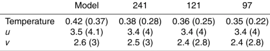
Table 2. RMS values compared to the Argo data for the area presented in Fig. 14 and four

simulations. In parenthesis values are shown calculated for north of 60◦_S.

Model 241 121 97

Temperature 0.42 (0.37) 0.38 (0.28) 0.36 (0.25) 0.35 (0.22)

u 3.5 (4.1) 3.4 (4) 3.4 (4) 3.4 (4)

(26)

OSD

8, 1535–1573, 2011

estimates

T. Janji´c et al.

Title Page

Tables Figures

◭ ◮

Back Close

Full Screen / Esc

Discussion

P

a

per

|

Dis

cussion

P

a

per

|

Discussion

P

a

per

|

Discussio

n

P

a

per

|

Fig. 1.Pre-Geoid corrections for GOCO01s and ITG-Grace03s gravity fields for Gaussian filter

(27)

OSD

8, 1535–1573, 2011

estimates

T. Janji´c et al.

Title Page

Tables Figures

◭ ◮

Back Close

Full Screen / Esc

Discussion

P

a

per

|

Dis

cussion

P

a

per

|

Discussion

P

a

per

|

Discussio

n

P

a

per

(28)

OSD

8, 1535–1573, 2011

estimates

T. Janji´c et al.

Title Page

Tables Figures

◭ ◮

Back Close

Full Screen / Esc

Discussion

P

a

per

|

Dis

cussion

P

a

per

|

Discussion

P

a

per

|

Discussio

n

P

a

per

|

Fig. 3. DOT from TOPEX, Jason-1, GFO, and ENVISAT obtained from data within ten day

(29)

OSD

8, 1535–1573, 2011

estimates

T. Janji´c et al.

Title Page Abstract Introduction Conclusions References Tables Figures ◭ ◮ ◭ ◮ Back Close

Full Screen / Esc

Printer-friendly Version Interactive Discussion Discussion P a per | Dis cussion P a per | Discussion P a per | Discussio n P a per −60˚ −60˚ −30˚ −30˚ 0˚ 0˚ 30˚ 30˚ 60˚ 60˚ −1 −0.5 −0.5 0 0 0.5 1

−1.5 m −1.0 m −0.5 m 0.0 m 0.5 m 1.0 m 1.5 m

−60˚ −60˚ −30˚ −30˚ 0˚ 0˚ 30˚ 30˚ 60˚ 60˚ −1.5 −1 −0.5 −0. 5 0 0 0.5 0.5 1 1

−1.5 m −1.0 m −0.5 m 0.0 m 0.5 m 1.0 m 1.5 m

MDOT2004 150 −60˚ −60˚ −30˚ −30˚ 0˚ 0˚ 30˚ 30˚ 60˚ 60˚ −1.5 −1−0.5 −0.5 0 0 0.5 0.5 1 1 1

−1.5 m −1.0 m −0.5 m 0.0 m 0.5 m 1.0 m 1.5 m

MDOT2004 180 −60˚ −60˚ −30˚ −30˚ 0˚ 0˚ 30˚ 30˚ 60˚ 60˚ −1.5 −1−0.5 −0.5 0 0 0.5 0.5 1 1 1

−1.5 m −1.0 m −0.5 m 0.0 m 0.5 m 1.0 m 1.5 m

Fig. 4. Mean DOT obtained using geodetic approach with Jekeli-Wahr filter with half width of

(30)

OSD

8, 1535–1573, 2011

estimates

T. Janji´c et al.

Title Page

Tables Figures

◭ ◮

Back Close

Full Screen / Esc

Discussion

P

a

per

|

Dis

cussion

P

a

per

|

Discussion

P

a

per

|

Discussio

n

P

a

per

|

GOCO01s JW241.6667km − ITG−Grace03s

−60˚ −60˚

−30˚ −30˚

0˚ 0˚

30˚ 30˚

60˚ 60˚

−1.0 cm −0.5 cm 0.0 cm 0.5 cm 1.0 cm

GOCO01s (JW 120.8333km − 241.6667km)

−60˚ −60˚

−30˚ −30˚

0˚ 0˚

30˚ 30˚

60˚ 60˚

−6 cm −4 cm −2 cm 0 cm 2 cm 4 cm 6 cm

GOCO01s (JW 96.6667km − 120.8333km)

−60˚ −60˚

−30˚ −30˚

0˚ 0˚

30˚ 30˚

60˚ 60˚

−1.0 cm −0.5 cm 0.0 cm 0.5 cm 1.0 cm

GOCO01s (JW 80.5556km − 96.6667km)

−60˚ −60˚

−30˚ −30˚

0˚ 0˚

30˚ 30˚

60˚ 60˚

−1.0 cm −0.5 cm 0.0 cm 0.5 cm 1.0 cm

Fig. 5. The difference between mean geodetic DOTs obtained from GRACE data only and

by combining GRACE and GOCE gravity data with both filtered using Jekeli-Wahr filter with

half width of 241 km (upper left). The difference between geodetic DOTs obtained combining

GRACE and GOCE gravity data filtered up to degree 241 km and 121 km (upper right), filtered up to degree 121 km and 97 km (lower left), filtered up to degree 97 km and 81 km (lower right).

(31)

OSD

8, 1535–1573, 2011

estimates

T. Janji´c et al.

Title Page

Tables Figures

◭ ◮

Back Close

Full Screen / Esc

Discussion

P

a

per

|

Dis

cussion

P

a

per

|

Discussion

P

a

per

|

Discussio

n

P

a

per

GOCO01s (JW 120.8333km − 241.6667km)

−60˚ −60˚

−30˚ −30˚

0˚ 0˚

30˚ 30˚

60˚ 60˚

−15 cm2 _{−10 cm}2 _{−5 cm}2 _{0 cm}2 _{5 cm}2 _{10 cm}2 _{15 cm}2

GOCO01s (JW 96.6667km − 120.8333km)

−60˚ −60˚

−30˚ −30˚

0˚ 0˚

30˚ 30˚

60˚ 60˚

−15 cm2 _{−10 cm}2 _{−5 cm}2 _{0 cm}2 _{5 cm}2 _{10 cm}2 _{15 cm}2

Fig. 6.Difference in temporal variance for 2004 between half width 241 km and 121 km filtering

(32)

OSD

8, 1535–1573, 2011

estimates

T. Janji´c et al.

Title Page

Tables Figures

◭ ◮

Back Close

Full Screen / Esc

Discussion

P

a

per

|

Dis

cussion

P

a

per

|

Discussion

P

a

per

|

Discussio

n

P

a

per

|

Fig. 7. Evolution of RMS error of SSH for the world ocean. The black lines with bullets

repre-sent the 10-day model forecasts, while the dotted gray lines correspond to the analysis. RMS error for assimilation of data filtered up to half width of 121 km and localization function that

correspond to Gaussian with length scale 246 km (900 km cutoff) (left). RMS error for

assim-ilation of data filtered up to half width of 121 km and localization function that corresponds to

(33)

OSD

8, 1535–1573, 2011

estimates

T. Janji´c et al.

Title Page

Tables Figures

◭ ◮

Back Close

Full Screen / Esc

Discussion

P

a

per

|

Dis

cussion

P

a

per

|

Discussion

P

a

per

|

Discussio

n

P

a

per

MDOT analysis

−60˚ −60˚

−30˚ −30˚

0˚ 0˚

30˚ 30˚

60˚ 60˚

−1

−0.5 0

0

0.5 1

1

−1.5 m −1.0 m −0.5 m 0.0 m 0.5 m 1.0 m 1.5 m

MDOT forecast

−60˚ −60˚

−30˚ −30˚

0˚ 0˚

30˚ 30˚

60˚ 60˚

−1

−0.5 0

0

0.5 1

1

−1.5 m −1.0 m −0.5 m 0.0 m 0.5 m 1.0 m 1.5 m

Fig. 8.Mean DOT obtained as the result of analysis (upper) and forecast (lower). An example of

assimilation of data filtered up to half width of 121 km and localization function that correspond