under the Inflation Targeting Regime:
Commitment vs. Discretion
Andreza Aparecida Palma
∗
, Marcelo Savino Portugal
†
Contents: 1. Introduction; 2. Theoretical Model; 3. Data Description; 4. Results; 5. Conclusion; A. Results of Model Estimation Using the Monetary Conditions Index (MCI).
Palavras-chave: Inflation Target, Central Bank Preferences, Central Bank of Brazil, Kalman Filter. Códigos JEL: C61; E52; E58.
This work aims to estimate the preferences of the Central Bank of Brazil during the inflation targeting regime, using a standard new key-nesian model with forward-looking expectations, as proposed by Gi-vens (2010). The presence of rational expectations in the model makes a distinction between two modes of optimization, commitment and discretion, and thus allows us to evaluate which of these specifications is favored by the data. Using quarterly data for the period from 2000-1 to 2010-4, the obtained results allow us to affirm that the data favor a discretionary policy. Estimates of the loss function show that the mo-netary authority gives great weight to inflation stabilization, followed by interest rate smoothing and stabilization of the output gap.
O objetivo principal deste trabalho é estimar as preferências do Banco Central do Brasil durante o regime de metas de inflação, usando um modelo novo-keynesiano padrão com expectativasforward-looking, conforme pro-posto por Givens (2010). A consideração de expectativas racionais separa as políticas em dois casos possíveis, regras e discrição e, portanto, permite avaliar com qual desses dois casos os dados são mais consistentes. Usando observações trimestrais, para o período de 2000-1 a 2010-4, os resultados obtidos permitem afirmar que, para o período considerado, os dados fa-vorecem uma política discricionária. As estimativas da função perda reve-lam que a autoridade monetária dá um grande peso para a estabilização
∗Assistant Professor of Economics at Universidade Federal de São Carlos (UFSCAR) and PhD Student in Economics at Universidade
Federal do Rio Grande do Sul (UFRGS). Rodovia João Leme dos Santos (SP-264), km. 110 – CEP 18052-780 – Bairro do Itinga – Sorocaba – São Paulo. E-mail:[email protected]
†Professor of Economics at both Graduate Program in Business Administration (PPGA) and Graduate Program in Economics
(PPGE) at Universidade Federal do Rio Grande do Sul. Av. João Pessoa, 52 sala 33B – 3◦andar – CEP 90040-000 – Centro – Porto
da inflação, seguida pela suavização da taxa de juros e pela estabilização do hiato do produto.
1. INTRODUCTION
The Taylor rule, which empirically describes the monetary authority’s response to macroeconomic variables, has been the standard tool used to assess the behavior of central banks over the past few decades. Even though this rule was proposed from a thoroughly empirical standpoint, there also exists a theoretical basis, which offers the solution to a constrained optimization problem through which the central bank minimizes a quadratic loss function.1 This way, the coefficients estimated in a reaction function are rather complex combinations of preference parameters (objective function coefficients) of the monetary authority with structural parameters of the model. Therefore, the coefficients obtained for the reaction function are reduced-form estimates and do not describe the structural characteristics of the monetary policy, having no use in assessing issues relative to the monetary policy formulation process.
Having information about the preferences of the central bank is of utmost importance. Several episodes of inflation, for instance, can be triggered by the monetary authority’s attempt to stabilize the output above its natural rate. Moreover, the larger the relative weight of output on the loss function, the larger the inflationary bias towards the economy. According to Castelnuevo e Surico (2003, p. 336), knowing the preferences of the central bank makes it possible to assess its performance more accurately, as it allows determining whether the result obtained is the one actually pursued by the central bank or whether it is just a random gain from favorable macroeconomic conditions.
There are numerous studies that have sought to estimate the preferences of central banks world-wide, especially for the US (Federal Reserve– FED). Among them, we cite Ozlale (2003) and Favero e Rovelli (2003), which estimate versions of the purely backward-looking model devised by Rudebusch e Svensson (1999), using the maximum likelihood method and the generalized method of moments (GMM), respectively. Applying a calibration strategy, Söderlind et alii (2002) and Castelnuevo e Surico (2003) find the relative weights for the FED’s preferences. Bearing in mind forward-looking models, we can cite the one developed by Ilbas (2008), which uses a DSGE model and Bayesian methods to estimate the FED’s preferences, taking into account a commitment environment. Dennis (2004) utilizes a new Keynesian model with a fully discretionary policy. These studies conclude that the FED pays greater importance to interest rate smoothing and lesser or insignificant importance to the output gap.
In Brazil, Aragon e Portugal (2009) were the first (and, to our knowledge, the only ones) to analyze the monetary authority’s preferences. In a calibration exercise of the loss function, these authors use a backward-looking model and choose preference parameter values that minimize the deviation between the simulated optimal trajectory and the true trajectory of the Selic rate. Given that in a calibration exercise, inference would not be possible, they use the optimal structure to estimate the preferences by maximum likelihood. Their results indicate that the Central Bank of Brazil gives the inflation rate a heavier weight and that the preoccupation with interest rate smoothing is greater than with the output gap. Note, however, that in the maximum likelihood estimation, the loss function parameters were insignificant. This, as explained by the authors, may have occurred because of the small sample size used.
In light of the facts mentioned above, gaining a better understanding of the monetary authority’s preferences in Brazil, mainly during the inflation targeting regime, is fundamental. Our goal is to es-timate these preferences in a more robust manner. We are going to use a standard new Keynesian model with forward-looking expectations, as proposed by Givens (2010). The structure of the economy is modeled by an IS and a Phillips curve. As far as rational expectations are concerned, it is necessary
to make a key distinction about how the agents’ expectations are dealt with in the optimization prob-lem, that is, to tell commitment and discretion apart, as pointed out by Kydland e Prescott (1977) and Barro e Gordon (1983). The major difference between the two possibilities lies in the way how agents’ expectations are dealt with in the central bank’s optimization problem.
In a commitment environment, the optimization of the monetary authority occurs only once and the effects of its choices will be internalized in the agents’ expectations. Conversely, in a discretionary policy regime, the monetary authority reoptimizes its loss function in each and every period, taking the agents’ expectations as given. Unlike other studies that estimate the preferences of the central bank using forward-looking models, no given policy (commitment×discretion) will be determined for the estimation process. Actually, based on the data and on the estimation of the two possible cases, we can decide which is more plausible. The main objective here is to estimate the monetary authority’s preferences and to verify which case is more compatible with the current monetary policy framework.
It should be noted that the inflation targeting regime is a tool that enhances transparency, commu-nication, and coherence of the monetary policy and that does not necessarily consist of a traditional rigid system of rules (Bernanke e Mishkin, 1997). As a matter of fact, this regime is compatible with the discretionary behavior of the monetary policy. According to Mendonça (2001), the transparency of the inflation targeting regime enables the use of discretionary policies without the monetary authority losing its credibility.
Thus, the present paper innovates by using a forward-looking model that is more consistent with the optimization and rational expectations approaches, making it a one-of-a-kind piece of work for the Brazilian case. The forward-looking behavior stresses the central role in expectations formation, especially under the inflation targeting regime, highlighting the importance of future events in relation to current ones. This will help improve the understanding of monetary policy conduct in Brazil during the inflation targeting regime, correcting some flaws of previous studies dealing with the same topic.
The remainder of the paper is organized as follows. Section 2 introduces the theoretical model, al-lowing for the estimation of the monetary authority’s preferences, and the estimation method. Section 3 describes the dataset. Section 4 presents the results of the paper and Section 5 concludes. The ap-pendix contains the same model used in main body of the article but the monetary policy instrument is assumed to be the MCI (monetary conditions index).
2. THEORETICAL MODEL
To estimate the preferences, we follow Givens (2010). The structure of the economy is represented by a standard new Keynesian model, which consists of two equations (IS and Phillips curve) that are used as constraint on the monetary authority’s optimization problem. The IS curve contains backward-looking and forward-backward-looking terms and is represented by equation (1) below. The new Keynesian Phillips curve is given by equation (2).
yt = φEtyt+1+ (1−φ) (βyt−1+ (1−β)yt−2)−σ(it−Etπt+1) +uy,t (1) πt = αEtπt+1+ (1−α)πt−1+κyt+uπ,t (2)
In IS equation (1),ytis the output gap (i.e., the log of the deviation between the real and the
poten-tial output),πtis the inflation rate between(t−1)and(t), itis the short-term nominal interest rate, uy,tis a non-autocorrelated demand shock, with zero mean and constant varianceσ2y(e.g., government
spending),σis the intertemporal elasticity of substitution in consumption (which measures the impact of changes in the real interest rate on the current output), φ ∈ [0,1]measures the forward-looking behavior of the agents’ spending decisions.
Fuhrer e Rudebusch, 2004) and theoretically as well, owing to habit formation in consumption (Fuhrer, 2000). In fact, as demonstrated in Givens (2010), an IS equation with the same lag structure can be derived from a general equilibrium model with habit formation. The same lag structure was found by Aragon e Portugal (2009) for the Brazilian case using the correlogram method.
The Phillips curve follows Galí e Gertler (1999). It is a hybrid new keynesian Phillips curve where a fraction of the economic agents do not set prices in optimal framework. Therefore uπ,t is a
non-autocorrelated supply shock, with zero mean and constant varianceπ2
π, which can be interpreted as
a cost-push shock, that is, variations in the marginal cost that do not affect the output gap (Clarida et alii, 1999). The parameter α ∈ [0,1]measures how much monopolistically competitive firms are forward-looking in their pricing decisions. Ifα= 1, we have the new Phillips curve estimated by Galí e Gertler (1999), which is consistent with a model of monopolistically competitive firms and sticky prices, according to Calvo (1983). If firms have the chance to reprice, they maximize their profits restricted to the probability of subsequent changes in prices. The key factor that influences the pricing decisions of firms is the real marginal cost, which varies proportionally to the output gap (Woodford, 2003a). Ifα < 1, (2) includes an inertial term, which supports the empirical evidence that inflation has a slow reaction to economic shocks. Fuhrer e Moore (1995), Fuhrer (1997) and Roberts (1997) state that, without this inertial behavior, the model would generate a dynamics with “jumps”, running counter to the empirical evidence. Theoretically, this inclusion can be justified by the presence of non-optimizing firms, which choose prices automatically indexed to the past inflation2or by the existence of a set of firms that use a given rule of thumb for price determination, which depends on the recent price history (Galí e Gertler, 1999). The restriction that the coefficients of the past and future inflation add up to 1 ensures that the Phillips curve given by (2) is compatible with the fact that the monetary policy does not have a long-term effect on output.
The slope coefficientκ > 0provides information about the frequency of price revisions. There-fore, the larger the nominal rigidity (i.e., the less frequent the revisions), the smaller the value of this parameter.
In addition, the model allows for the correlation between supply and demand shocks, with covari-ance given byσyπ.
2.1. Central bank and the optimal monetary policy rule
The intertemporal loss function of the monetary authority is given by equation (3). The monetary authority’s objective is therefore to minimize (3) subject to the restrictions given by (1) and (2).
Lt=Et(1−δ) ∞ X
j=0 δjnπ2
t+j+λyyt+j2 +λ△i(it+j−it+j−1) 2o
(3)
whereδis the intertemporal discount rate andEtis the expectation operator conditional on the set of
data available at time andλy,λ△i>0are the parameters related to the central bank preferences.
The quadratic loss function given in (3) is commonly used in the literature. The monetary authority is assumed to be in charge of stabilizing the annualized inflationπt+jaround the inflation target. Note,
however, that the inflation target is time-invariant and is therefore normalized to zero, as all variables in the model are expressed as deviations from the mean. As shown in Dennis (2006), this does not change the derivation of central bank preferences. In addition to seeking to stabilize inflation, the monetary authority is also concerned with output stabilization (represented in the equation by output gapyt+j) and with interest rate smoothing, last term of equation (3). The output target is its potential
level.
The monetary authority’s preference parameters for output gap stabilization and interest rate smooth-ing are given relative to the inflation stabilization weight, besmooth-ing normalized to unit. As the sum of the weights of each of the three variables of the loss function adds up to one, it is possible to obtain the absolute weights from the relative weights.
The choice of a quadratic loss function is quite attractive and is generally used in the related liter-ature. According to Aragon e Portugal (2009), this is due to three main reasons. First, this quadratic function combined with linear restrictions produces linear policy rules. Second, a function like this allows for the inclusion of the nominal interest rate smoothing term. Finally, loss functions such as (3), but without the interest rate smoothing term, can be derived from a second-order approximation of the intertemporal utility function of the representative agent,3which provides a welfare criterion for the classification of alternative policies. Moreover, as (3) is commonly used in the literature, the estimated parameters can be easily interpreted and it is possible to compare them with previous results. Accord-ing to Svensson (1996), the major goal of a central bank that adopts the inflation targetAccord-ing regime can be described by a loss function which stabilizes inflation and by a measure of real activity.
The inclusion of the interest rate smoothing term has received massive empirical support in the lit-erature, despite the difficulty in providing a theoretical explanation. Note that the interest rate smooth-ing term is used here to capture the preference for reducsmooth-ing the variance of the first difference of the nominal interest rate.4 The preference for gradual movements in this variable may be explained by a number of reasons. For example, abrupt changes in the interest rate can destabilize the financial and exchange rate markets (Lowe e Ellis, 1997). Furthermore, according to Woodford (2003b), in forward-looking models, the interest rate inertia is typical of an optimal inflation target rule.
Details on the model solution and estimation procedures are omitted here, but can be found Givens (2010).
3. DATA DESCRIPTION
Quarterly data for the Brazilian economy in the post-target period (January 2000 – December 2010) will be used, totaling 44 observations of the following variables:
• Output gap: percentage deviation of the seasonally adjusted real GDP from the potential GDP (calcu-lated through the Hodrick-Prescott filter).
• Annualized inflation rate (IPCA): IPCA over 12 months (percentage variation). Quarterly mean. Source: IBGE
• Nominal interest rate (1st difference): annualized Selic rate. Quarterly mean. Source: BCB – Sisbacen.
The stationarity of the series used was checked by Dickey-Fuller and Phillips-Perron tests, whose results are shown below. It may be concluded that the series are stationary at a 5% significance level. It is important to note that we use the interest rate in first difference, since it is non-stationary in the Brazilian case. Nevertheless, one may argue that the monetary policy instrument is the interest rate itself (Selic target). We test both possible ways of introducing the interest rate in the model (in level and in first difference). The results were not substantially different. Therefore we preferred to use the stationary series.5
According to the literature, the variables for inflation rate and nominal interest rate were calculated as deviation from the sample means. This is interesting for two reasons. The major goal of the paper
3About this latter argument, see Woodford (2003a).
4Some works use this same term to denote a reaction function in which the coefficient of the lagged interest rate is substantially
greater than zero (Givens, 2010).
Table 1: Unit root tests
Variable ADF test Phillips-Perron test (pvalue) (pvalue) Output gap -4.635629 -2.283105
(0.0005) (0.0232) Inflation -2.249315 -1.969038
(0.0253) (0.0478) Interest rate -5.812382 -2.651965 (1st difference) (0.0000) (0.0092)
is to estimate the preferences of the central bank and to compare the fit of the model under commit-ment and discretion, instead of obtaining the estimates for the central bank’s implicit targets for these variables. In addition, this procedure produces the same inflation targets and interest rate for both optimization cases. The choice for quarterly observation of the data, a gold standard in the related lit-erature, seeks to minimize problems with measurement errors and to reduce the number of lags in the model, as the effects of the monetary policy actions on inflation take two or three semesters to appear.
4. RESULTS
The model was estimated using the Matlab6software and the results are shown in Tables 2 and 3 for the commitment and discretion cases, respectively. Table 4 shows the comparison of fit measures between the two models: log-likelihood, Bayesian information criterion and pseudo-posterior odds. The latter measure shows the probability of a given model conditional on data. The variances were calculated from elements of the diagonal of the information matrix.
The comparison between the models shown in Table 4 allows us to state that the data are more consistent with the discretionary policy for the analyzed period. Therefore, the central bank’s behav-ior would not be limited to promises made in previous periods. In Brazil, the targets are adjustable (flexible), that is, they can be changed in the presence of adverse shocks. At first sight, this result may seem undesirable because, according to Kydland e Prescott (1977), discretionary policies would reduce the welfare of society at large. However, a more recent strand of the literature demonstrates that a rule-based policy could be inferior to a discretionary one. For instance, Sauer (2007) concludes that if an economy is characterized by sticky prices, low discount factor, large preference for output stabilization or if it is far enough from its steady state, a discretionary policy could be preferable over one that is based on commitment.
The parameters of both models (discretion and commitment) are very much alike, except for the preference parameters. As to IS and Phillips curves, it should be noted that the forward-looking and backward-looking components are rather significant and important, but the backward-looking term is superior to the forward-looking only in the IS curve. The intertemporal elasticity of substitution in consumption(σ)is quite small in both models, which may indicate smoothed consumption, as the larger the elasticity, the smaller the risk aversion. Low values for this coefficient concur with those of some other empirical studies that estimate this parameter for the Brazilian economy.7 The results also
6The routines were kindly granted by Gregory Givens.
Table 2: Model estimated under commitment
Parameters Estimate Std deviation Pvalue (Wald test)
σy 0.2009 0.059697 0.00076453
σπ 0.7 0.017149 0.00000000
σyπ -0.052482 0.05826 0.30307311 σi 1.05 0.008352 0.00000000 λy 0.19 0.026733 0.00000000 λ△i 20.005 0.05142 0.00000000 φ 0.2500 0.023453 0.00000000
β 1.300 0.15602 0.00000000
σ 0.0500 0.057155 0.38167506
α 0.6500 0.003757 0.00000000
κ 0.0001 0.04105 0.99805631
Absolute weights:λ′
y= 0.0596 λ′△i= 0.6270 λ
′
π= 0.3134
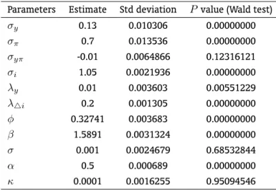
Table 3: Model estimated under discretion
Parameters Estimate Std deviation Pvalue (Wald test)
σy 0.13 0.010306 0.00000000 σπ 0.7 0.013536 0.00000000 σyπ -0.01 0.0064866 0.12316121 σi 1.05 0.0021936 0.00000000 λy 0.01 0.003603 0.00551229 λ△i 0.2 0.001305 0.00000000 φ 0.32741 0.003683 0.00000000
β 1.5891 0.0031324 0.00000000
σ 0.001 0.0024679 0.68532844
α 0.5 0.000689 0.00000000
κ 0.0001 0.0016255 0.95094546
Absolute weights:λ′
y= 0.0083 λ′△i= 0.1653 λ
′
π= 0.8264
Table 4: Comparison between the models
show the importance of both the forward-looking and backward-looking components in the Phillips curve. The small estimation value for parameterκ, although not statistically significant, implies large nominal price rigidity. With respect to the estimates of covariance, the demand shocks are more volatile than supply shocks in both models. On the other hand, the estimate ofσi reveals that the difference
between the optimal policy given by the model and the observed policy is invariant in both models. The preference parameters of the central bank markedly differ between the two behaviors of the monetary authority. Under commitment, interest rate smoothing is more important, followed by in-flation, while little attention is paid to output stabilization. This significant difference between the two models is due to the fact that there is an increase in interest rate volatility under commitment, causing the maximum likelihood method to make up for this effect by placing a heavier weight on the parameter that captures the interest rate smoothing, in order to fit the model to the data (Givens, 2010). In the discretionary policy, we have a heavier weight on inflation stabilization, followed by interest rate and output stabilization. The results obtained by Aragon e Portugal (2009) showed a larger weight on inflation than on other variables (albeit not statistically significant), but a smaller weight than that attributed in the present paper to the discretionary policy. Thus, it may be concluded that the Central Bank of Brazil gives inflation stabilization a larger weight, but that it does not rule out output stabi-lization or interest rate smoothing. The lesser weight on output stabistabi-lization implies a low inflationary bias in the analyzed period. The results are quite plausible in economic terms, given that the major objective of the monetary authority is inflation stabilization. In addition, the monetary authority’s concern with output exists only because its stabilization helps control inflation. The concern with in-terest rate smoothing is also consistent with the fact that the central bank does not adjust the nominal interest rate at once in response to changes in economic fundamentals.
5. CONCLUSION
The present paper sought to estimate the monetary authority’s preferences using a standard new keynesian model in which the monetary authority minimizes an intertemporal loss function subject to economic restrictions given by IS and Phillips curves, using rational expectations. Considering the forward-looking nature of the model, it is necessary to make a distinction between the two approaches (commitment and discretion) to the optimization problem. In the discretionary policy, optimization occurs in each and every period. Under commitment, however, it occurs only once. This way, it is possible to determine which case is more compatible with the dataset by using some fit measures.
The model was estimated using quarterly data (to minimize measurement errors and the number of lags) in the post-target period (2000-1 to 2010-4). The results allow asserting that the data are favorable to the discretionary policy. The monetary authority assigns a large weight on inflation stabilization, but it also takes into account interest rate smoothing and output stabilization. Albeit small, the weights on output stabilization and interest rate smoothing are statistically different from zero. This result is quite plausible in economic terms, as the main goal of the monetary authority is inflation stabilization. Moreover, the monetary authority’s concern with output only exists because its stabilization helps control inflation.
The results show that the Central Bank of Brazil adopts a flexible inflation targeting regime com-patible with a discretionary policy, which is also comcom-patible with the monetary authority’s behavior observed during the period. In some instances, such as in 2002, the inflation target to be followed was changed, but this change was not announced to the public at an early stage. According to Mendonça (2001), because of the transparency of the inflation targeting regime, it is possible to use discretionary policies without affecting the credibility of the monetary authority. The discretionary policy adopted in the period is therefore compatible with the findings of previous studies that indicate an improvement in the credibility of the Central Bank of Brazil under the inflation targeting regime.8
BIBLIOGRAFIA
Aragon, E. K. & Portugal, M. S. (2009). Central bank preferences and monetary rules under the inflation targeting regime in Brazil. Brazilian Review of Econometrics, 29(1):79–109.
Barro, R. J. & Gordon, D. B. (1983). A positive theory of monetary policy in a natural rate model.Journal of Political Economy, 91(4):589–610.
Bernanke, B. & Mishkin, F. (1997). Inflation targeting: A new framework for monetary policy? Journal of Economic Perspectives, 11(2):97–116.
Calvo, G. A. (1983). Staggered prices in a utility maximizing framework. Journal of Monetary Economics, 12(3):383–398.
Castelnuevo, E. & Surico, P. (2003). What does monetary policy reveal about a central bank’s preferences?
Economic Notes, 32(3):335–359.
Christiano, L. J., Eichenbaum, M., & Evans, C. L. (2005). Nominal rigidities and the dynamic effects of a shock to monetary policy. Journal of Political Economy, 113(1):1–45.
Clarida, R., Galí, J., & Gertler, M. (1999). The science of monetary policy: A new keynesian perspective.
Journal of Economic Literature, 37(4):1661–1707.
Dennis, R. (2004). Inferring policy objectives from economic outcomes.Oxford Bulletin of Economics and Statistics, 66(S1):735–764.
Dennis, R. (2006). The policy preferences of the US Federal Reserve. Journal of Applied Econometrics, 21(1):55–77.
Estrella, A. & Fuhrer, J. C. (2002). Dynamic inconsistencies: Counterfactual implications of a class of rational-expectations models. The American Economic Review, 92(4):1013–1028.
Favero, C. A. & Rovelli, R. (2003). Macroeconomic stability and the preferences of the Fed: A formal analysis,1961-98.Journal of Money, Credit and Banking, 35(4):545–556.
Fuhrer, J. C. (1997). The (un)importance of forward-looking behavior in price specifications. Journal of Money, Credit and Banking, 29(3):338–350.
Fuhrer, J. C. (2000). Habit formation in consumption and its implications for monetary-policy models.
The American Economic Review, 90(3):367–390.
Fuhrer, J. C. & Moore, G. R. (1995). Inflation persistence. The Quarterly Journal of Economics, 110(1):127– 159.
Fuhrer, J. C. & Rudebusch, G. D. (2004). Estimating the Euler equation for output. Journal of Monetary Economics, 51(6):1133–53.
Galí, J. & Gertler, M. (1999). Inflation dynamics: A structural econometric analysis. Journal of Monetary Economics, 44(2):195–222.
Givens, G. (2010). Estimating central bank preferences under commitment and discretion. Working Paper Middle Tennessee State University.
Issler, J. V. & Piqueira, N. S. (2000). Estimating relative risk aversion, the discount rate and the in-tertemporal elasticity of substitution in consumption for Brazil using three types of utility function.
Brazilian Review of Econometrics, 20(2):201–239.
Kydland, F. E. & Prescott, E. C. (1977). Rules rather than discretion: The inconsistency of optimal plans.
Journal of Political Economy, 85(3):473–491.
Lowe, P. & Ellis, L. (1997). Smoothing of official interest rates. In Lowe, P., editor,Monetary Policy and Inflation Targeting, pages 286–312. Reserve Bank of Australia.
Mendonça, H. (2001). Mecanismos de transmissão monetária e a determinação da taxa de juros: Uma aplicação da regra de Taylor ao caso brasileiro.Economia e Sociedade, 16:65–81.
Ozlale, U. (2003). Price stability vs. output stability: Tales of federal reserve administrations. Journal of Economic Dynamics and Control, 17(9):1595–1610.
Palma, A. A. & Portugal, M. S. (2009). Análise empírica da formação de expectativas de inflação no Brasil: Uma aplicação de redes neurais artificiais a dados em painel. Revista de Economia Contemporânea, 13(3):391–437.
Roberts, J. M. (1997). Is inflation sticky? Journal of Monetary Economics, 39(3):173–196.
Rudebusch, G. D. & Svensson, L. E. (1999). Policy rules for inflation targeting. In Taylor, J. B., editor,
Monetary Policy Rules. The University of Chicago Press, Chicago.
Sauer, S. (2007). Discretion rather than rules? When is discretionary policy-making better than the timeless perspective? European Central Bank Working Paper Series, 717.
Smets, F. & Wouters, R. (2003). An estimated dynamic stochastic general equilibrium model of the Euro area.Journal of European Economic Association, 1(5):1123–1175.
Söderlind, P., Söderström, U., & Vredin, A. (2002). Can calibrated new-keynesian models of monetary policy fit the facts? Stockholm: Sveriges Riksbank, Working paper 140.
Svensson, L. E. O. (1996). Inflation forecasting targeting: Implementing and monitoring inflation targets. Cambridge: National Bureau of Economic Research (Working Paper 5797).
Woodford, M. (2003a).Interest and Prices: Foundations of a Theory of Monetary Policy. Princeton University Press, New Jersey.
A. RESULTS OF MODEL ESTIMATION USING THE MONETARY CONDITIONS INDEX (MCI)
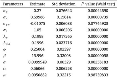
In trying to consider the influence of exchange rate on the inflation and on the setting the interest rate by the Central Bank the model was also estimated using the MCI as the monetary policy instrument. The MCI is weighted average to interest rate and exchange rate. In a way it also means that the Central Bank cares about both inflation and exchange rate dynamics. The MCI weights were extracted from a price equation. The estimated results are presented in the following tables. This is a simple way of trying to acknowledge that exchange rate dynamics may be more relevant for the Central Bank of Brazil then to the FED.
Table A.1. Model estimated under commitment – MCI (commitment)
Parameters Estimate Std deviation Pvalue (Wald test)
σy 0.75 0.053486 0.00000000 σπ 0.05 0.009775 0.00000031 σyπ -0.07 0.030558 0.02197928 σi 0.1 0.008404 0.00000000 λy 0.0001 0.050411 0.99841724 λ△i 0.05 0.001888 0.00000000
φ 0.6 0.025929 0.00000000
β 1.25 0.18713 0.00000000
σ 0.08964 0.020271 0.00000978
α 0.3500 0.032744 0.00000000
κ 0.001 0.041091 0.98058441
Absolute weights:λ′
y= 0.0001 λ′△i= 0.0476 λ
′
π= 0.9523
Table A.2. Model estimated under discretion – MCI (commitment)
Parameters Estimate Std deviation P value (Wald test)
σy 0.27 0.076642 0.00042690 σπ 0.69986 0.15614 0.00000739 σyπ -0.01075 0.006088 0.07744928 σi 1.05 0.006206 0.00000000 λy 0.1998 0.017365 0.00000000 λ△i 0.1996 0.023716 0.00000000 φ 0.25004 0.02397 0.00000000
β 15.996 0.32008 0.00000058
σ 0.0099949 0.00329 0.00238183
α 0.56066 0.006558 0.00000000
κ 0.0050882 0.32215 0.98739833
Absolute weights:λ′
y= 0.1428 λ′△i= 0.1426 λ
′
Table A.3. Comparison between the models
Model Log-likelihood BIC Pseudo-odds Commitment -422.43 -443.243 2.92E-67 Discretion -269.23 -290.043 1.00