Saturation in autoregressive models

(1)

(2)

8

9

Neste artigo estendemos a ideia base do algorítmo de saturação de modelos com variáveis indicadores a um tipo particular de modelos dinâmicos. Demonstra-se que o procedimento mantém o nível de significância real correcto para processos AR(1) estacionários, independentemente do número de partições da amostra usado. Derivamos a potência teórica em face de um outlier de tipo aditivo e apresentamos evidência de Monte Carlo que demonstra uma boa taxa de rejeição empírica da hipótese nula nesse caso. É apresentado um conjunto extenso de simulações de Monte Carlo que

evidenciam que o procedimento tem uma potência apreciável quando existe quebra na média condicional do processo nas últimas rT% observações da amostra. Este resultado não depende do nível de autocorrelação das observações, nem da utilização de um mal especificado modelo do tipo location-scale, abrindo assim as portas a uma nova classe de testes automáticos de quebras de estrutura que poderão revelar-se melhores que testes do tipo de Bai-Perron em pequenas amostras.

resumo résumé / abstract

Carlos Santos1_{/ David Hendry}2

1_{Portuguese Catholic University, FEG /}2_{University of Oxford, Department of Economics}

Saturation in Autoregressive Models

In this paper, we extend the impulse satura-tion algorithm to a class of dynamic models. We show that the procedure is still correctly sized for stationary AR(1) processes, inde-pendently of the number of splits used for sample partitions. We derive theoretical power when there is an additive outlier in the data, and present simulation evidence show-ing good empirical rejection frequencies against such an alternative. Extensive Monte Carlo evidence is presented to document that the procedure has good power against a level shift in the last rT%of the sample observa-tions. This result does not depend on the level of serial correlation of the data and does not require the use of a (mis-specified) loca-tion-scale model, thus opening the door to an automatic class of break tests that could out-perform those of the Bai-Perron type. JEL Codes: C22; C51

(3)

A key recent development in testing for parameter non-constancy is doing so by adding a complete set of indicators to a model (see Hendry, Johansen and Santos, 2005). This new technique came to be known as impulse or indicator saturation. Using general-to-specific (GETS) procedures, the authors establish the null distribution of the mean and variance estimators in a location-scale model, after adding Timpulses, when Tis the sample size, and retaining the relevant ones. A two-fold process is investigated whereby half the indicators are added and the significant ones recorded. Then, the other half is examined, and finally the two are combined in a union model. Under the null hypothesis that no indicator matters, the average retention rate of indicators is αT, matching the binomial result exactly, and showing that there is no overfitting3_. Moreover, Hendry at al. (2005) show that other splits (such as T/3, T/4, etc) do not affect the retention rate of the model under the null.

Hendry and Santos (2006) extend this procedure to break testing in location-scale models. What under the null was a model selection problem, under the alternative becomes a test for breaks at unknown dates, since an indicator is tested for every observation. Theoretical power of the impulse saturation break test is derived, both for the case of a mean shift and for the case of a variance shift. Results are shown to be remarkably close to Monte Carlo outcomes.

Previous results on GETS model selection where there are more candidate indicator variables than indicators are given in Hendry and Krolzig (2003). Notwithstanding, the theoretical analysis for the general case treated there is hardly as developed as the analysis in Hendry et al. (2005) for the case of a complete set of indicators. Clearly, the reason for this is that impulse dummies are perfectly orthogonal to each others, so we do not have to cope with the problems of collinearity faced in more general settings (see Hendry and Krolzig (2003), and Hendry and Castle (2005)). Hendry (2000) advises orthogonalization of the regressors prior to model selection as a way to reduce model uncertainty.

The objective of this paper is to extend the baseline impulse saturation results to a class of dynamic models, namely that of stationary autoregressive models. We provide Monte Carlo evidence that there are no size distortions in impulse saturating stationary autoregressive processes, and that the procedure has good power properties in this class of models both to detect additive outliers (AO) and to detect level shifts at unknown dates.

The paper is organized as follows. Section 2 presents Monte Carlo evidence of the null rejection frequencies (NRFs) of indicators in saturated stationary AR(1) models. A pilot extension to a unit root process is also documented. Section 3 derives analytical power of the procedure for the additive outlier case, and compares such results with Monte Carlo evidence. Section 4 provides simulation results for rejection frequencies of the null when there is a level shift on the last of the sample observations. Section 5 concludes.

1. Introduction

1 Corresponding Author: csantos@porto.ucp.pt . Universidade Católica Portuguesa, Faculdade de Economia e Gestão, Rua Diogo Botelho 1327, 4169-005 Porto. Phone contact: 00351226196200, ext. 180.

2 This research was conducted while the first author was a doctoral student at the University of Oxford, UK, and is a part of his doctoral dissertation. Both authors acknowledge the invaluable contributions of Soren Johansen and Bent Nielsen in several discussions. Several participants at the Royal Economic Society Annual Conference 2006 provided useful comments and suggestions. James Reade provided invaluable research assistance. The authors are also most grateful for comments by the Editor and an anonymous referee. The usual disclaimer applies. Financial Support from the Fundação para a Ciência e a Tecnologia, Lisbon, and from the ESRC under a Professorial Fellowship, RES051270035, are acknowledged by the first and second authors respectively. 3 Hendry, Leamer and Poirier (1990) conclude that the tests have the same properties at each reduction stage as when applied in the General Unrestricted Model. Hence, there is no need to adjust critical values for testing in the union model. White (1991) and Mayo (1980) corroborate this. In particular Mayo (1980) argues that test information is independent from sufficient statistics from which parameter estimates are derived.

(4)

We consider the stationary AR (1) process with zero mean as the Data Generating Process (DGP):

(1) We assume that ε_t~ IN(0;1) and that |r| <1. We consider adding Timpulses in partitions of T/2 and T/3 to (1). Hence, the two General Unrestricted Models (GUMs) would be the DGP

augmented by T/2 indicators, in the first case studied. In the second case, the three GUMs would match (1) augmented with T/3 indicators.

That is, for T/2we consider the intermediate econometric models:

and

A partition of T/3would naturally imply three intermediate regressions.

We allow rto vary across the Monte Carlo experiments, taking values from 0.1 to 0.9. The objective of considering this range for the autoregressive parameter is to check if the null properties of the model depend on the degree of first order serial correlation in the sample. The sample sizes considered are T = 100, T= 200 and T = 3005_{. Individual significance tests on} the impulse indicators are conducted for a range of significance levels α, taking values from the set {0.1; 0.05; 0.025; 0.01}6_.

It should be noticed that the computed t-ratios are constructed using the standard normal approximation to the distribution of the individual significance test statistics. M = 10000 replications are conducted in each experiment and the empirical rejection frequency is the average across all experiments of the ratio of indicators retained in the union model to the sample size. Table 1 reports the results for T = 300 and a split of T/2.

10

11

4 All the Monte Carlo simulations conducted in this paper were written using Ox 3.4 (Doornik, 2001). In particular, autoregressive series were generated using the armagen function within the ARMA package. All codes written for this paper are available from the authors on request.

5 In practice we have generated samples of sizes 120, 220 and 320 and we have disregarded the first 20 observations in each case, in order to eliminate dependence on the initial values.

6 Santos (2006) shows the results are not sensitive to changes to in the innovation variance.

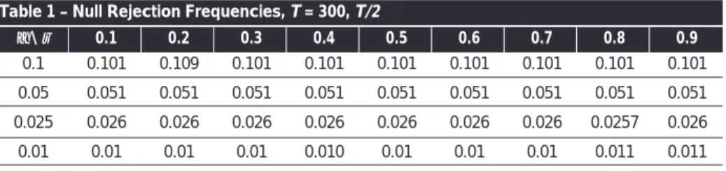
Table 1 – Null Rejection Frequencies, T = 300, T/2

0.1 0.05 0.025

0.01

2. Null Rejection Frequencies in the Impulse Saturated Stationary AR(1) Process4

α\ ρ 0.101 0.051 0.026 0.01 0.1 0.109 0.051 0.026 0.01 0.2 0.101 0.051 0.026 0.01 0.3 0.101 0.051 0.026 0.010 0.4 0.101 0.051 0.026 0.01 0.5 0.101 0.051 0.026 0.01 0.6 0.101 0.051 0.026 0.01 0.7 0.101 0.051 0.0257 0.011 0.8 0.101 0.051 0.026 0.011 0.9

(5)

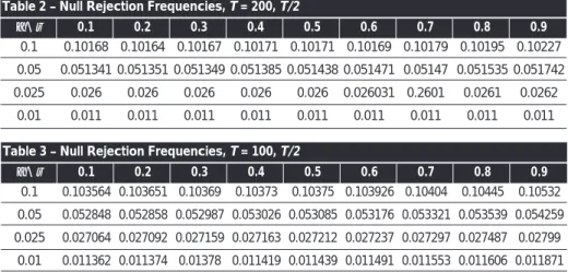
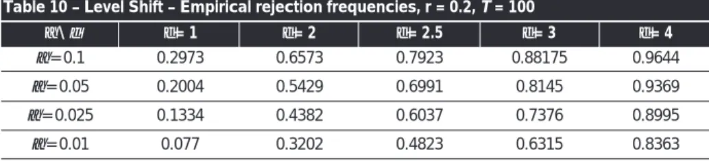
Table 1 shows that for such a sample size, the nominal significance level is close to the empirical rejection frequency: the two are never apart by more than two tenths of a percentage point. Table 2 refers to the T= 200 case. Again the split considered is T/2. In spite of the reduction in the sample size, the empirical rejection frequency is still close to the nominal significance. Table 3 reports the results for the case T= 100. Nominal and real significance levels diverge as the sample size decreases, as was to be expected given the asymptotic approximation used. Nonetheless, for T= 100, such a divergence is still small: in nearly all cases never greater than four tenths of a percentage point.

0.1 0.05 0.025 0.01 α\ ρ 0.10168 0.051341 0.026 0.011 0.1 0.10164 0.051351 0.026 0.011 0.2 0.10167 0.051349 0.026 0.011 0.3 0.10171 0.051385 0.026 0.011 0.4 0.10171 0.051438 0.026 0.011 0.5 0.10169 0.051471 0.026031 0.011 0.6 0.10179 0.05147 0.2601 0.011 0.7 0.10195 0.051535 0.0261 0.011 0.8 0.10227 0.051742 0.0262 0.011 0.9

0.1 0.05 0.025 0.01 α\ ρ 0.103564 0.052848 0.027064 0.011362 0.1 0.103651 0.052858 0.027092 0.011374 0.2 0.10369 0.052987 0.027159 0.01378 0.3 0.10373 0.053026 0.027163 0.011419 0.4 0.10375 0.053085 0.027212 0.011439 0.5 0.103926 0.053176 0.027237 0.011491 0.6 0.10404 0.053321 0.027297 0.011553 0.7 0.10445 0.053539 0.027487 0.011606 0.8 0.10532 0.054259 0.02799 0.011871 0.9

0.1 0.05 0.025 0.01 α\ ρ 0.10072 0.050676 0.0255 0.010299 0.1 0.10073 0.050676 0.025487 0.010295 0.2 0.10074 0.050671 0.025474 0.010306 0.3 0.10076 0.050691 0.025465 0.010291 0.4 0.10082 0.050697 0.025454 0.010295 0.5 0.10081 0.050694 0.025447 0.010308 0.6 0.10085 0.050716 0.025439 0.01029 0.7 0.10092 0.050746 0.025439 0.0103 0.8 0.10091 0.050789 0.025537 0.010347 0.9

0.1 0.05 0.025 0.01 α\ ρ 0.10118 0.05096 0.025689 0.010533 0.1 0.10123 0.050947 0.025725 0.01053 0.2 0.010114 0.051013 0.025726 0.010533 0.3 0.10117 0.051028 0.025726 0.010554 0.4 0.010119 0.051061 0.025698 0.010552 0.5 0.10119 0.051083 0.025726 0.010537 0.6 0.10127 0.051092 0.025748 0.010537 0.7 0.10134 0.051124 0.025781 0.010562 0.8 0.10157 0.05117 0.025885 0.01059 0.9 Tables 1, 2 and 3 also confirm that divergence between nominal and real significance levels are slightly more pronounced as ρbecomes closer to unity. In any case, the fundamental conclusion from the three tables is that nominal and real significance levels are close, overcoming most of the effects introduced by dynamics.

We now turn to investigate the impact of a different sample split on the empirical rejection frequency, under the null. The same defaults apply. Table 4 refers to the T= 300 case and table (5) to the T= 100.

(6)

As was already the case with the Monte Carlo evidence in the IID location-scale model, the change in the split from T/2 to T/3 does not alter the main result that nominal and real significance levels are close for the sample sizes considered.

In conclusion, the Monte Carlo analysis conducted suggests that it is possible to implement impulse saturation algorithm in a stationary AR(1) model, under the null hypothesis of no indicators in the DGP. NRFs distortions are, for the sample sizes considered, very small.

2.1. Rejection Frequency under the null: Unit Root Case

We have also run a pilot experiment to check whether there would be any significant NRFs problems in a random walk model. We considered the DGP:

(2) We assume that ε_t~ IN(0;1). Hence there are no dummies in the DGP, but there is a unit root. We consider the average across the Monte Carlo replications of the ratio of retained indicators to the sample size, at each replication as our measure of empirical NRFs. Results are reported on table 6 and confirm closeness of nominal and empirical NRFs. T/2 is used.

12

13

Table 6 – Null Rejection Frequencies Unit Root Case, T/2

0.1 0.05 0.025 0.01 α\ T 0.10402 0.052895 0.027025 0.011227 T = 300 0.106 0.054478 0.028076 0.011949 T = 200 0.11056 0.058025 0.030874 0.0113675 T = 100

Although there is a slight increase in the discrepancy between real and nominal sizes, at all significance levels, it is our view that these are not sufficient to preclude the saturation of a unit root model like (2). Nonetheless, the analysis of the unit root case would require considerable more evidence, whilst all we are doing here is to suggest that it would be possible to use dummy saturation in such models as well.

3.1 Monte Carlo evidence on power

In order to evaluate the use of a GETS modelling strategy for the inclusion of indicators in a stationary AR(1), we shall look at the problem under H₁, that is when the indicator’s coefficient of some impulse is not zero. We shall do this by imposing an additive outlier in the DGP, that is now given by:

(3)

where we assume that ε_t~ IN(0;1) and that |ρ| <1. Hence, at t= t* there is an additive outlier. We assume that this is an exogenous shock to y_t*such that,

(4)

(7)

In our Monte Carlo experiments, we allow to take values from the set {2; 2.5; 3; 4; 5}. Furthermore, it is known that the additive outlier has an effect in two periods in the residuals of the stationary AR(1) model: t*and t*+ 1. If the effect of the additive outlier at the time when it occurs is δ, on the following period it has an effect ρδ. Hence, for the relevant impulse indicators’ coefficients estimators to be unbiased they should have expectations equal to δand -ρδ. For |ρ| <1, this means that the second coefficient is smaller than the first in absolute value: the individual significance test statistics will have lower non-centralities implying lower power (see the analysis of theoretical power in the next subsection).

Table 7 reports the empirical rejection frequencies of the null, for the indicator at t*, when the sample size is T = 100, and an additive outlier occurs at T = 80. A significance level of 0.025 is used for impulse saturation, and the split is T/2. Table 8 refers to the t*+ 1 indicator.

7 Additional evidence as to the unbiasedness of the indicators’ coefficients in the two periods and as to the positive effect from impulse saturation, reducing the bias of ρ^, could also be given and is available upon request.

Table 7 – AO: Empirical Rejection Frequencies for the indicator at t*, T = 100, T/2 δ= 2 δ= 2.5 δ= 3 δ= 4 δ\ ρ 0.4063 0.6013 0.7729 0.9574 0.1 0.4057 0.6017 0.7721 0.9578 0.2 0.4065 0.6014 0.7726 0.958 0.3 0.4066 0.6009 0.7726 0.9577 0.4 0.4069 0.6011 0.7728 0.9571 0.5 0.4055 0.6012 0.7729 0.9564 0.6 0.4056 0.6005 0.7748 0.9559 0.7 0.4041 0.6013 0.7741 0.9562 0.8 0.4031 0.6001 0.771 0.9556 0.9

Table 8 – AO: Empirical Rejection Frequencies for the indicator at t* + 1, T = 100, T/2 δ= 2 δ= 2.5 δ= 3 δ= 4 δ\ ρ 0.033 0.0375 0.0418 0.0507 0.1 0.0432 0.0489 0.0597 0.0848 0.2 0.0574 0.0732 0.0943 0.1419 0.3 0.0782 0.1069 0.1419 0.232 0.4 0.1067 0.1532 0.211 0.3526 0.5 0.1429 0.2128 0.2996 0.4853 0.6 0.1902 0.2879 0.3985 0.6238 0.7 0.2464 0.3691 0.5086 0.754 0.8 0.3079 0.4616 0.6207 0.8589 0.9

The method appears to have good power to detect the moment at which the AO occurs. Power at that moment does not depend on the autoregressive coefficient, as was expected. Also, we confirm that the second indicator will be retained less often, with the autoregressive coefficient playing a role here7_.

3.2. Theoretical power derivation for the Additive Outlier case

We shall proceed with the analysis of theoretical power separating conclusions for the indicator at time t*and at time t*+1. Consider the DGP defined by (3) and (4), where |ρ| <1, ε_t~ IN(0;1). Consider the econometric model:

(5) D_tis a single impulse indicator such that D_t*= 1. d_tis another single impulse indicator such that d_t*+1= 1.

Suppose we wish to test the null hypothesis:

H

₀

:

ψ = 0

(8)

in a model that differs from (5) because it does not contain the lagged dummy (for simplicity). We make use of the test statistic:

(see Hendry and Santos, 2005). Hence,

Notice that:

Since,

and

we obtain,

which simplifies to:

14

(9)

Notice also that,

Under the alternative,

where χ2 _(1;_δ2_{) is a non-central}_χ2_{distribution with 1 degree of freedom and non-centrality} parameter δ2_{(see Johnson, Kotz and Balakrishnan, 1995).}

Bearing in mind that the relationship, between a non-central and a central χ2 _{with m}_{degrees of} freedom is given by:

(see Hendy, 1995), where,

and

for a significance level of 0.025, we can compute the probability of rejecting the null when indeed that is false as:

(6) The noticeable conclusion is that the non-centrality depends only on δ, and not on the sample size Tnor on the autoregressive coefficient ρ. This is line with our findings in table 7. Hence, for δ

∈ {2; 2.5; 3; 4} the values for theoretical power are

(7)

The Monte Carlo evidence reported on the relevant table of the previous subsection suggests that empirical power is always below theoretical power, but that the difference is never too big: about 0.1 for 2 ≤δ≤ 3, and vanishing rapidly for δ> 3.

(10)

3.3 Dummy at t + 1 when AO is at t

In this case,

(8) Hence, the noncentrality, and therefore power, will now depend both on δand on ρ. Suppose ρ = 0.9 and δ ∈ {2; 2.5; 3; 4}. Then, for a similar critical value as above,

(9)

Results should be compared with those in table 9. Again empirical power converges to theoretical power as δincreases.

16

17

Any reference to the power properties of impulse saturation algorithm in stationary

autoregressions, under the alternative, would have to contemplate both outliers and level shifts. In a sense, however, the analysis is not all that different, since level shifts are sequences of additive outliers (see Peña, 2001). Hence, we expect the impulse saturation algorithm to have power against level shifts in this class of models.

For the purpose of the Monte Carlo analysis we postulate a DGP where, for T ≤T*: (10) and for T >T*,

(11) where ε_t~ IN(0;1) and |ρ| <1. By assumption, . That is, the break occurs for the last 20% sample observations. In the first set of Monte Carlo results reported in tables 10-12, we assume that ρ= 0.5. Keeping ρand rfixed, we allow for different significance levels and break magnitudes. Tables 10-12 report the empirical null rejection frequencies for the indicators covering those last observations. The entire break period is comprised within a single partition. T/2is used.

Results reported in tables 10-12 are encouraging: empirical null rejection frequencies for the indicators in the break period indicate useful power for δ≥ 2.5, and α≥ 0.025. The sample size is

Table 9 – Theoretical power at time t + 1 δ= 2 δ= 2.5 δ= 3 δ= 4 δ\ ρ 0.3079 0.4616 0.6207 0.8589 0.9

(11)

not playing a relevant role here. A complete study should also allow rto vary. Nonetheless, this is not the main effect we are interested in studying here.

Table 10 – Level Shift – Empirical rejection frequencies, r = 0.2, T = 100 α= 0.1 α= 0.05 α= 0.025 α= 0.01 0.2973 0.2004 0.1334 0.077 0.6573 0.5429 0.4382 0.3202 α\ δ δ= 1 δ= 2 δ= 2.5 δ= 3 δ= 4 0.7923 0.6991 0.6037 0.4823 0.88175 0.8145 0.7376 0.6315 0.9644 0.9369 0.8995 0.8363

Table 13 – Level Shift – Empirical rejection frequencies, r = 0.2, T = 300, ρ= 0.9 α= 0.1 α= 0.05 α= 0.025 α= 0.01 0.093 0.157 0.23 0.3324 0.364 0.4825 0.585 0.693 α\ δ δ= 1 δ= 2 δ= 2.5 δ= 3 δ= 4 0.512 0.6343 0.725 0.811 0.65 0.7524 0.825 0.888 0.829 0.892 0.931 0.961

Rather we investigate whether the impulse saturation procedure is sensitive to the degree of serial correlation in the series. That is, instead of ρ= 0.5, as in the previous example, we shall be considering empirical power when ρ= 0.9. Therefore, we considered the following DGP:

(12) where ε_tis a Gaussian white noise process with unit variance, and δ ∈{1; 2; 2.5; 3; 4}. Table 13 reports results for a sample size of T = 300 and table 14 reports results for T = 100. Other defaults apply.

(12)

18

19

Comparing with the corresponding tables for ρ= 0.5, it is clear that there is no significant dominating power loss when ρis increased to 0.9. Indeed, in some cases power is even increased. This is an important result as it suggests power of this procedure does not depend on degree of serial correlation of the data.

In this paper we have established that the impulse saturation method can also be applied to stationary AR(1) models. Monte Carlo evidence has shown that nominal and real size are close for this type of model. There are some indications that the magnitude of the autoregressive coefficient and that the sample size might cause some deviations but these are, in any case, always very slight. A pilot extension to a unit root process suggests the process could be applied there as well.

On the other hand, impulse saturation tests are shown to have power (in the AR(1) framework) against additive outliers and level shifts. Theoretical power is studied for the AO case, whilst results for the level shift case are entirely simulation-based. In any event, the empirical rejection frequencies for the indicators at the AO date, or covering the shift period, indicate the procedure has good power against these alternatives.

A most relevant conclusion of this paper is that the impulse saturation test for level shifts in dynamic models does not depend on the degree of serial correlation of the sample, nor does it seem to demand that the test is conducted in a (mis-specified) location scale model. Hence there appears to be some advantages of using this procedure over the Bai and Perron test (1998, 2003). Santos (2006) explores this issue further.

The analysis developed here has already proven to be useful for the development of new super exogeneity tests (see Hendry and Santos, 2006a), and follows from the preliminary papers by Hendry, Johansen and Santos (2005) where the properties of the impulse saturation algorithm under the null that no indicators matter were studied in detail in a location-scale model, and Hendry and Santos (2006b) where it the power properties of the procedure in location-scale models were studied. Santos and Oliveira (2006) and Santos (2006) have developed empirical applications of these procedures.

Table 14 – Level Shift – Empirical rejection frequencies, r = 0.2, T = 100, ρ= 0.9 α= 0.1 α= 0.05 α= 0.025 α= 0.01 0.147 0.227 0.309 0.413 0.465 0.574 0.665 0.759 α\ δ δ= 1 δ= 2 δ= 2.5 δ= 3 δ= 4 0.604 0.708 0.784 0.8553 0.717 0.83 0.8623 0.913 0.858 0.909 0.941 0.966 5. Conclusions

(13)

Bai, J.; Perron, P. (1998) Estimating and Testing Linear Models with Multiple Structural Changes, Econometrica, 66, 47-78.

Bai, J.; Perron, P. (2003) Computation and Analysis of Multiple Structural Change Models, Journal of Applied Econometrics, 18, 1-22.

Doornik, J. A. (2001) OX – An Object Oriented Matrix Programming Language, London, Timberlake Consultants.

Hendry, D. F. (2000) Econometrics, Alchemy or Science?, Oxford, Oxford University Press. Hendry, D. F. (1995) Dynamic Econometrics, Oxford, Oxford University Press.

Hendry, D. F.; Castle, J. L. (2005) A low dimension collinearity robust test for non-linearity, Unpublished Paper, Department of Economics, University of Oxford,

Hendry, D. F.; Krolzig, H.-M. (2003) Sub-Sample Model Selection Procedures in GETS Modelling, paper presented at the ESAM,

Hendry, D. F.; Santos C. (2005) Regression Models with Data-Based Indicator Variables, Oxford Bulletin of Economics and Statistics, 67, 5, 571-595

Hendry, D. F.; Santos, C. (2006a) Automatic Super Exogeneity Tests, Univeristy of Oxford, Department of Economics, Unpublished Paper.

Hendry, D. F.; Santos C. (2006b) On the Power of Impulse Saturation Break Tests, Unpublished Paper, University of Oxford, Department of Economics.

Hendry, D. F.; Leamer, E. E.; Poirier, D. J. (1990) The ET Dialogue: a Conversation on Econometric Methodology, Econometric Theory, 6, 2, 171-261.

Hendry, D. F.; Johansen, S.; Santos, C. (2005) Selecting a Regression Saturated with Indicators, University of Oxford, Department of Economics, Unpublished Paper.

Johnson, N. L.; Kotz, S.; Balakrishnan, N. (1995) Continuous Univariate Distributions —2, 2nd edition, New York: John Wiley and Sons.

Mayo, D. (1981) Testing Statistical Testing, in Pitt, J. C. (ed.), Philosophy in Economics, 175-230, D. Reidel Publishing Co.

Santos, C. (2006) Structural Breaks and Outliers in Economic Time Series, D.Phil. Thesis, Univeristy of Oxford.

Santos, C.; Oliveira, M. A. (2006) Modelling the German Yield Curve and Testing the Lucas Critique, mimeo.

Peña, D. (2001) Outliers, Influential Observations and Missing Data, in Peña, D., Tiao, G. C. and Tsay, R. S. (eds.), A Course in Time Series Analysis, Wiley Series in Probability and Statistics, New York: John Wiley and Sons.

Santos (2006) Structural Breaks and Outliers in Economics Time Series: Modelling and Inference, D.Phil. Thesis, University of Oxford, Department of Economics.

White, H. (1990) A Consistent Model Selection Procedure based on M-testing, in Granger, C. W. J. (ed.), Modelling Economic Series, 369-383, Oxford: Clarendon Press.

(14)