Brazilian Journal of Physics, vol. 36, no. 3A, September, 2006 623
Monte Carlo Simulations of a
Semi-Flexible Polymer Chain: A First Glance
D. T. Seaton, S. J. Mitchell, and D. P. Landau
Center for Simulational Physics, University of Georgia, Athens, GA 30602, USA
Received on 23 December, 2005
We present preliminary results for Monte Carlo simulations of a three dimensional semi-flexible polymer chain with continuous monomer positions. In these simulations, standard Metropolis Monte Carlo methods are used to examine the basic properties of the model, such as equilibration configurations, overall size, and transition temperatures.
Keywords: Monte Carlo simulations; Polymer chain
I. INTRODUCTION
There are many examples of polymer systems, ranging in complexity from strands of DNA and protein molecules to ex-amples of simple plastics. Regardless of the level of com-plexity, the three dimensional structure of a polymer chain will determine many of its most important properties. Monte Carlo methods have shown great promise in studying polymer conformation problems [1]. In particular, a wide variety of Monte Carlo methods have been applied to single chain poly-mer systems that include flexibility[2–4]. Many of these types of studies consider the bond fluctuation model [5], in which the monomer positions are confined to a lattice. Through the use of a polymer model with continuous monomer positions, we hope to add more realism to the study of general poly-mer conformation problems. In this preliminary work, we concentrate on understanding the basic features of our poly-mer model, such as equilibration time, overall size of equili-brated configurations, and location of transition temperatures. In particular, we examine the transition between folded and unfolded states.
II. MODEL
The polymer model consists of a chain of N identical monomers, where each monomer position varies continuously in three dimensions. There are three types of interactions: a harmonic bond length interaction between nearest neighbor bonded monomers, a bond angle interaction between adjacent bonds, and a non-bonded interaction between all non-bonded monomers. The Hamiltonian for this model is
H
=JL N−1∑
i(li−1)2+JA N−2
∑
i(cos(θi) +1)2+JNB
∑
i,jf(ri j) (1) whereN is the number of monomers, JL is the bond length interaction parameter,liis theith bond length, where the pre-ferred bond length isli=1.0, and∑N−i 1 is the sum over all N−1 bonds. In the second term,JAis the bond angle inter-action parameter, ∑N−i 2 is the sum over all N−2 bond an-gles, andθiis the angle between adjacent bonds, which has a preferred bond angle ofθi=180. In the third term,JNBis
0
1
2
3
r
-1
0
1
2
3
Potential Energy
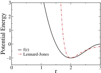
f(r)Lennard-JonesFIG. 1: Plot comparing the non-bonded interaction potential, f(r), to a Lennard-Jones potential.
the non-bonded interaction parameter,∑i,jis the sum over all non-bonded pairs of monomers, and f(ri j)is the non-bonded interaction potential, whereri j is the distance between two non-bonded monomers. The function f(r)represents a quasi-Lennard-Jones potential [6] and is intended to model variable solvent quality [7, 8]. This function is given by
f(r) = ½
3(r−2)2
−2(r−2)3−1, for 0<r<3,
0, otherwise, (2)
where the minimum of this function is atr=2. Fig. 1 com-paresf(r)to a standard Lennard-Jones potential, showing that f(r)has a softer repulsion as monomers come closer together. We work in reduced units, in whichJNB=1, andJLandJA can be varied. For the current study we examine the behavior of the model for
JL=30,JA=30,JNB=1. (3) Initial simulations indicated that whenJLis too small(∼1),
624 D. T. Seaton et al.
(Folded) T = 1.0
(Unfolded) T = 5.0
FIG. 2: Above we see a folded configuration at a low temperature and an unfolded configuration at a high temperature, each with a chain length ofN=40. In these models, spheres represent monomers, and cylinders represent bonds between monomers.
III. METHOD
In simulating the polymer model, standard Metropolis Monte Carlo methods [9] have been used. Changes are made to the polymer configurations using the following types of moves: monomer diffusion, reptation, crank-shaft, and ran-dom pivot. One Monte Carlo sweep (MCS) consists of N attempted monomer diffusion moves and a single attempt of each of the other types of moves. A monomer diffusion move randomly selects a monomer, and then displaces it a random distance within a small cubic volume. A reptation move ran-domly selects one monomer from either end of the chain and then reattachs it to the opposite end of the chain. A crank-shaft move randomly selects two non-bonded monomers and then rotates the portion of the chain between those monomers by a small random angle. A random pivot move randomly selects a single monomer and the portion of the connected chain on either side of the monomer. A random direction is then cho-sen and the selected portion of the chain is then rotated around this random axis by a small random angle.
To characterize the behavior of the polymer, we observe quantities such as the radius of gyration and the average en-ergy per particle. These two quantities offer much insight into the general properties of the polymer model, such as config-uration types and equilibration time. Energies,E/N, are cal-culated using Eq. 1, and the radius of gyration is calcal-culated using
Rg= s
∑Ni (~ri−~rcm)2
N (4)
where~ri is theith monomer position, and~rcm is the position of the center of mass. The radius of gyration represents the overall size of the polymer chain. For a given N, low values of Rgrepresent more compact folded configurations, and higher values ofRgrepresent unfolded configurations.
0 50 100 150 200 250
t [10
3MCS]
1.5 2 2.5 3 3.5 4
R
gN = 25 N = 40 N = 80
0 50 100 150 200 250
t[10
3MCS]
-6 -5 -4 -3 -2 -1 0 1
E / N
N = 25 N = 40 N = 80 T = 1.0
T = 1.0
Brazilian Journal of Physics, vol. 36, no. 3A, September, 2006 625
0 50 100 150 200 250
t [10
3MCS]
1.5 2 2.5 3 3.5 4 4.5 5
R
gN = 25 N = 80
0 50 100 150 200 250
t [10
3MCS]
-5 -4 -3 -2 -1 0 1 2 3
E / N
N = 25 N = 80 T = 2.0
T = 2.0
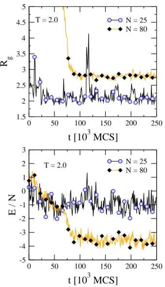
FIG. 4: Similar to Fig. 3 but forT =2.0. TheN=40 series has been removed for clarity. Symbols are added every 104MCS point, to help distinguish the three curves.
IV. SIMULATION RESULTS
Typical simulations ran between 105and 106MCS, when starting from a straight configuration. In each simulation,Rg andE/Nare calculated after each MCS. For the following re-sults, radius of gyration and energy per particle are reported every 103MCS. The chain size in these simulations was usu-ally in the range ofN=25 toN=80, however, simulations have been run for sizes up toN=256. Typical configurations for aN=40 chain can be seen in Fig. 2. The first chain rep-resents a folded configuration at a low temperature (T=1.0), and the second chain represents an unfolded configuration at a higher temperature (T =5.0).
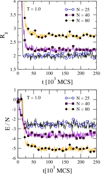
In Fig. 3 the radius of gyration and energy per particle are both plotted as functions of time for three different chain sizes, all at a low temperature (T=1.0). Symbols are added every 104MCS, to help distinguish the three curves. In this figure, each chain relaxes into a folded state, and at this temperature,
2 4 6 8 10
2 4 6 8
R
g0 200 400 600 800 1000
t [10
3MCS]
0 2 4 6 8
T = 4.0
T = 2.5
T = 1.0
N = 25
N = 25
N = 25
FIG. 5: Radius of gyration as a function of Monte Carlo time for a chain of lengthN=25, where each sequence shows the polymer fluctuating at a different temperature.
the relaxation time scale is much shorter than 2.5×10⁵MCS.
Fig. 4 is similar to Fig. 3 but shows data at a slightly higher temperature (T =2.0). TheN=40 curve has been removed for clarity. The principal feature in this figure is that fluctua-tions occur on time scales much larger than those atT=1.0. We see that the fluctuations in Fig. 3 are quite rapid on this time scale, but for T =2.0 in Fig. 4 fluctuations occur on much larger time scales. Another feature seen in this figure is that larger fluctuations occur for shorter chains.
626 D. T. Seaton et al.
0 2 4 6 8 10
T
0 0.2 0.4 0.6 0.8 1
<R
g
>
2 /N
N = 25 N = 40 N = 80
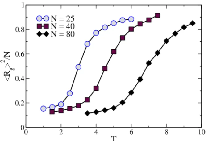
FIG. 6: Plots of squared and scaled average radius of gyration as a function of temperature for three different chain lengths, where the connecting lines are guides to the eye. When not shown, error bars are much smaller than the symbol size.
be related to the stiffnes of the chain. By exploring different values ofJA, we expect to achieve a better understanding of this apparent transition.
V. CONCLUSIONS
Using standard Monte Carlo methods, we have studied the basic properties of a semi-flexible polymer chain. Through the observation of such quantities as the radius of gyration and the energy per particle, we have been able to understand the basic physical behaviors of our polymer model. However, these standard Monte Carlo methods become inefficient for larger systems, creating a need for a faster sampling method. In the near future, we would like to increase the efficiency of our simulations through the application of Wang-Landau sampling [10–12] techniques. This will not only “speed up” our simulations, but it should also allow us to gain a better understanding of the model.
Acknowledgments
We thank W. Paul and F. Rampf for helpful discussions. This work is supported by NSF grants DMR-0307082 and DMR-0341874, and LLNL grant B551576.
[1] See e.g., K. Binder and A. Milchev, J. Comput. Aided Mater. Des.9, 33 (2002).
[2] M. Stukan, V. Ivanov, A. Y. Grosber, W. Paul, and K. Binder, J. Chem. Phys.118, 3392 (2003).
[3] F. Rampf, W. Paul, and K. Binder, Europhys. Lett. 70, 628 (2005).
[4] J. Martemyanova, M. Stukan, V. Ivanov, M. M ¨uller, W. Paul, and K. Binder, J. Chem. Phys.122, 174907 (2005).
[5] I. Carmesin and K. Kremer, Macromolecules21, 2819 (1988). [6] A. Milchev, W. Paul, and K. Binder, J. Chem. Phys.99, 4786
(1993).
[7] V. Ivanov, W. Paul, and K. Binder, J. Chem. Phys.109, 5659 (1998).
[8] V. Ivanov, M. Stukan, V. Vasilevskaya, and K. Binder, Macro-mol. Theory Simul.9, 488 (2000).
[9] D. P. Landau and K. Binder,A Guide to Monte Carlo Simula-tions in Statistical Physics(Cambridge University Press, New York, NY, 2000), ISBN 0-521-65366-5.