Oi
S.
A.
J
os
é
Sar
ment
o,
152110319
Advi
s
or
:
Pr
of
.
J
os
é
Car
l
os
T
udel
a
Marns
Di
s
s
er
t
aon
s
ubmied
i
n
paral
f
ul
fil
l
ment
of
r
equi
r
ement
s
f
or
t
he
degr
ee
of
MSc
i
n
Bus
i
nes
s
Admi
ni
s
t
r
aon,
at
t
he
Cat
ól
i
c
a
L
i
s
bon
Sc
hool
of
Bus
i
nes
s
&
Ec
onomi
c
s
,
J
anuar
y
2013
The company will struggle to successfully implement its new investment plan. On one hand I believe that the company is minimizing its Capex needs. On the other hand, the company is already highly leveraged and this program will increase further its financing needs.
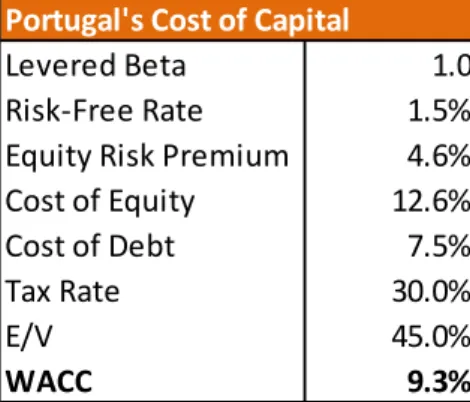
Both classes of shares deserve an underweight recommendation, with a price target of BRL7.38 for the Common and BRL5.47 for the Preferred shares for YE12. I have used a WACC of 12.8% for the Brazilian Operations.
The company should continue outperforming its peers, gaining market-share, both on Mobile as in the Residential sector. Its plan to start targeting high-customers has high risks, as it forces the company to continue investing on its infrastructures. On the other hand, this plan exposes the company to other risks. The company is the largest fixed line phone company in the country. Instead of leveraging its market position, if the company persists with its plan it could be neglecting the opportunity of pushing their fixed-line clients to Paid-TV. The corporate segment should also continue being negatively affected by increasing competition.
16 October 2012
Oi Common Target Price BRL7.38 Current Price BRL10.47
Oi Preferred Target Price BRL5.47 Current Price BRL8.46
Analyst: José Sarmento
0 20 40 60 80 100 120 140 160
Jan Feb Mar Apr May Jun Jul Aug Sep Oct
2012 YTD Stock Performance
Oi Preferred Oi Common Bovespa
Oi's Valuation - SoP
Oi Operations EV (BRL mn) 33,884.6 Net Debt (BRL mn) 25,369.4 Portugal Telecom (BRL mn) 1,436.7 Equity Value (BRL mn) 35,321.3 Target Price Oi BR4 (BRL) 5.47 Upside (Downside) -35.4% Target Price Oi BR3 (BRL) 7.38 Upside (Downside) -29.5% Source: Bloomberg
integrated operator in the country. Despite the weak economic backdrop, we believe that the position of Portugal Telecom should continue to be supported by its revenues resilience.
Oi: Summary of Financials
Oi's Total Revenues
BRL (mn) 2012 E 2013 E 2014 E 2015 E 2016 E 2017 E 2018 E 2019 E 2020 E Residential 9,913.4 10,454.3 10,830.8 11,227.6 11,624.3 11,918.7 12,217.1 12,519.6 12,826.2 Personal Mobility 8,941.3 9,843.7 10,641.4 11,541.9 12,478.9 13,399.5 14,315.3 15,169.8 15,878.0 Corporate 8,321.0 8,321.0 8,518.0 8,709.1 8,890.1 9,082.8 9,293.5 9,505.8 9,726.6 Others 581.4 546.5 513.7 482.9 453.9 426.7 413.9 401.4 389.4 Total 27,757.0 29,165.4 30,503.8 31,961.4 33,447.3 34,827.7 36,239.8 37,596.7 38,820.3 Oi's P&L BRL (mn) 2012 E 2013 E 2014 E 2015 E 2016 E 2017 E 2018 E 2019 E 2020 E
Net Operating Revenues 27,757.0 29,165.4 30,503.8 31,961.4 33,447.3 34,827.7 36,239.8 37,596.7 38,820.3
Operating Expenses 19,438.7 20,194.7 20,963.7 21,783.8 22,619.8 23,439.4 24,297.4 25,152.3 25,982.2
EBITDA Pro-Forma 8,318.3 8,970.7 9,540.1 10,177.6 10,827.5 11,388.3 11,942.3 12,444.4 12,838.1
EBITDA Consolidated 7,455.8 8,970.7 9,540.1 10,177.6 10,827.5 11,388.3 11,942.3 12,444.4 12,838.1
Depreciation and Amortization 4,222.1 4,832.2 5,029.4 5,238.4 5,446.8 5,648.0 5,816.5 5,936.8 5,997.3
EBIT 3,233.8 4,138.5 4,510.7 4,939.2 5,380.8 5,740.3 6,125.9 6,507.6 6,840.7
Net Financial Income -1,914.3 -1,966.1 -2,162.4 -2,348.1 -2,443.5 -2,596.0 -2,708.1 -2,772.4 -2,778.6
Average Cost of Debt 11.0% 7.8% 7.8% 7.8% 7.8% 7.8% 7.8% 7.8% 7.8%
EBT 1,319.4 2,172.4 2,348.3 2,591.1 2,937.3 3,144.3 3,417.8 3,735.2 4,062.1
Taxes 329.6 651.7 704.5 777.3 881.2 943.3 1,025.3 1,120.6 1,218.6
% Taxes 25.0% 30.0% 30.0% 30.0% 30.0% 30.0% 30.0% 30.0% 30.0%
Net Income before non-controlling shareholders 989.9 1,520.7 1,643.8 1,813.7 2,056.1 2,201.0 2,392.4 2,614.6 2,843.5
Non-Controlling Shareholders 6.3 6.3 6.3 6.3 6.3 6.3 6.3 6.3 6.3 Net Income 983.6 1,514.4 1,637.5 1,807.4 2,049.8 2,194.7 2,386.1 2,608.3 2,837.2 2012 E 2013 E 2014 E 2015 E 2016 E 2017 E 2018 E 2019 E 2020 E 6.102 6.476 6.771 6.974 7.123 7.052 6.819 6.441 6.095 OI: Estimated Capex Needs(BRL mn)
BRL (mn) 2012 E 2013 E 2014 E 2015 E 2016 E 2017 E 2018 E 2019 E 2020 E
Current Assets 18,615.2 18,813.7 19,709.5 20,746.3 22,616.3 22,331.4 21,902.1 22,206.2 23,165.1
Cash and Cash Equivalents 4,341.2 4,266.5 4,783.0 5,406.9 6,855.8 6,179.8 5,350.3 5,269.9 5,882.1
Financial Investments 2,325.0 2,325.0 2,325.0 2,325.0 2,325.0 2,325.0 2,325.0 2,325.0 2,325.0 Derivatives 160.0 160.0 160.0 160.0 160.0 160.0 160.0 160.0 160.0 Accounts Receivable 5,718.6 5,914.1 6,185.5 6,481.1 6,782.4 7,062.3 7,348.6 7,623.8 7,871.9 Recoverable Taxes 1,993.5 2,061.6 2,156.2 2,259.2 2,364.3 2,461.9 2,561.7 2,657.6 2,744.1 Inventories 278.9 288.5 301.7 316.1 330.8 344.5 358.5 371.9 384.0 Assets in Escrow 2,299.0 2,299.0 2,299.0 2,299.0 2,299.0 2,299.0 2,299.0 2,299.0 2,299.0
Other Current Assets 1,499.0 1,499.0 1,499.0 1,499.0 1,499.0 1,499.0 1,499.0 1,499.0 1,499.0
Non Current Assets 58,851.1 60,878.3 62,985.2 65,118.4 67,199.8 68,979.7 70,366.1 71,238.1 71,667.1
Long Term 18,428.3 18,808.9 19,170.7 19,564.6 19,966.1 20,339.2 20,720.8 21,087.5 21,418.2 Taxes 7,501.3 7,881.9 8,243.7 8,637.6 9,039.1 9,412.2 9,793.8 10,160.5 10,491.2 Financial Investments 62.0 62.0 62.0 62.0 62.0 62.0 62.0 62.0 62.0 Assets in Escrow 9,088.0 9,088.0 9,088.0 9,088.0 9,088.0 9,088.0 9,088.0 9,088.0 9,088.0 Derivatives 537.0 537.0 537.0 537.0 537.0 537.0 537.0 537.0 537.0 Other Assets 1,240.0 1,240.0 1,240.0 1,240.0 1,240.0 1,240.0 1,240.0 1,240.0 1,240.0 Investments 78.0 78.0 78.0 78.0 78.0 78.0 78.0 78.0 78.0 Fixed Assets 24,145.1 25,130.5 26,174.9 27,215.8 28,221.2 29,063.1 29,664.5 29,966.9 30,025.7
% of Intangible assets + Fixed Assets 60.0% 60.0% 60.0% 60.0% 60.0% 60.0% 60.0% 60.0% 60.0%
Intangible Assets 16,199.7 16,860.9 17,561.6 18,260.0 18,934.5 19,499.4 19,902.8 20,105.8 20,145.2
% of Intangible assets + Fixed Assets 40.2% 40.2% 40.2% 40.2% 40.2% 40.2% 40.2% 40.2% 40.2%
Total Assets 77,466.4 79,692.1 82,694.7 85,864.7 89,816.1 91,311.1 92,268.1 93,444.3 94,832.2
Current Liabilities 14,412.5 14,734.0 15,307.2 15,787.1 16,436.4 16,802.5 17,101.3 17,398.9 17,687.8
Suppliers 4,152.1 4,190.1 4,349.7 4,519.8 4,693.3 4,863.3 5,041.4 5,218.7 5,390.9
Loans and Financing 3,297.3 3,544.4 3,837.3 4,023.7 4,367.2 4,444.7 4,444.7 4,444.7 4,444.7
% of Gross Debt 10.3% 10.3% 10.3% 10.3% 10.3% 10.3% 10.3% 10.3% 10.3%
Financial Instruments 141.6 152.2 164.7 172.7 187.5 190.8 190.8 190.8 190.8
% of Gross Debt 0.4% 0.4% 0.4% 0.4% 0.4% 0.4% 0.4% 0.4% 0.4%
Others 6,821.6 6,847.3 6,955.5 7,070.8 7,188.4 7,303.7 7,424.4 7,544.6 7,661.3
Payroll and Related Accruals 535.0 539.9 560.5 582.4 604.7 626.7 649.6 672.5 694.6
Provisions 1,659.0 1,659.0 1,659.0 1,659.0 1,659.0 1,659.0 1,659.0 1,659.0 1,659.0
Taxes 2,279.6 2,300.4 2,388.0 2,481.4 2,576.7 2,670.0 2,767.8 2,865.2 2,959.7
Dividends 259.0 259.0 259.0 259.0 259.0 259.0 259.0 259.0 259.0
Other Accounts 2,089.0 2,089.0 2,089.0 2,089.0 2,089.0 2,089.0 2,089.0 2,089.0 2,089.0
Non-Current Liabilities 42,735.3 45,167.9 48,012.2 49,924.6 53,240.1 54,181.6 54,445.6 54,708.5 54,963.8
Loans and Financing 29,209.1 31,398.3 33,992.9 35,644.7 38,687.8 39,373.8 39,373.8 39,373.8 39,373.8
% of Gross Debt 91.00% 91.00% 91.00% 91.00% 91.00% 91.00% 91.00% 91.00% 91.00%
Financial Instruments 146.6 157.6 170.6 178.9 194.2 197.6 197.6 197.6 197.6
% of Gross Debt 0.5% 0.5% 0.5% 0.5% 0.5% 0.5% 0.5% 0.5% 0.5%
Taxes 5,979.5 6,212.1 6,448.7 6,700.9 6,958.1 7,210.2 7,474.1 7,737.1 7,992.4
Contigency Provisions 5,212.0 5,212.0 5,212.0 5,212.0 5,212.0 5,212.0 5,212.0 5,212.0 5,212.0
Provisions for the Pension Fund 446.0 446.0 446.0 446.0 446.0 446.0 446.0 446.0 446.0
Outstanding Authorizations 1,061.0 1,061.0 1,061.0 1,061.0 1,061.0 1,061.0 1,061.0 1,061.0 1,061.0
Other Accounts Payable 681.0 681.0 681.0 681.0 681.0 681.0 681.0 681.0 681.0
Total Liabilities 57,147.8 59,901.9 63,319.3 65,711.7 69,676.5 70,984.2 71,546.8 72,107.4 72,651.6
Shareholder's Equity 20,318.6 19,790.1 19,375.4 20,153.0 20,139.6 20,327.0 20,721.3 21,336.9 22,180.6
Controlling Interest 20,275.6 19,747.1 19,332.4 20,110.0 20,096.6 20,284.0 20,678.3 21,293.9 22,137.6
Minority Interest 43.0 43.0 43.0 43.0 43.0 43.0 43.0 43.0 43.0
Equity + Liabilities 77,466.4 79,692.1 82,694.7 85,864.7 89,816.1 91,311.1 92,268.1 93,444.3 94,832.2
FCFF Details - Domestic Operations
BRL (Mn) 2012 E 2013 E 2014 E 2015 E 2016 E 2017 E 2018 E 2019 E 2020 E Terminal value
EBITDA 8,318.3 8,970.7 9,540.1 10,177.6 10,827.5 11,388.3 11,942.3 12,444.4 12,838.1
Capex 6,102.4 6,475.7 6,771.3 6,974.4 7,123.5 7,052.1 6,819.3 6,441.2 6,095.5
Taxes 329.6 651.7 704.5 777.3 881.2 943.3 1,025.3 1,120.6 1,218.6
Change in working capital/other flows 1,997.1 357.5 236.7 269.2 274.4 226.7 219.1 190.6 133.2
1
Abstract
Valuation is a fundamental instrument of the Modern World. It provides one of the foundations of society, as it establishes what is fair and what it isn’t for a certain asset. In Equity Research, one of the major and most complex fields of Valuation we must value a company relative to its industry and geographic location while trusting the data it makes available. This Thesis intends to bridge the theory and the practice of Equity Valuation, valuing Oi’s Preferred and Common Shares. Oi is one of the major Telecom companies in Brazil. After my research I arrived at a fair value price of BRL5.47 and BRL7.38 for each, leading to an Underweight recommendation for both.
2
Preface
My path in Finance has been extremely demanding but, at the same time, extremely rewarding. For a competitive person like me, I am continuously motivated by the constant challenges I must face and the sense of victory each time I overcome them. On this path there are several people to whom I am very grateful – Professor Tudela Martins, for his availability and untiring support on the elaboration of this Thesis; to Ricardo Lourenço, for teaching me everything I know about Equity Research; to Albino Oliveira, my colleague and teacher who guides me every day; to Gonçalo and Pedro Pereira Coutinho for their confidence in me and the opportunities they provide me at FINCOR – SOCIEDADE CORRETORA, S.A.; to all my colleagues at FINCOR – SOCIEDADE CORRETORA, with whom I spend the majority of my time; to Paulo Silva and the rest of the Alumbrados Group, for every discussion we have about the markets and life in general, as in this sector it is almost impossible to separate the two; to Professors Paulo Gonçalves Marcos and Isabel Viegas for always believing in my potential; to Marília Cabral who provided my first introduction to the Investment Banking World and helped me to discover my professional vocation; to Michael Castelhano, Duarte Cabral and the rest of the Research Department in Banco Best, who were both colleagues and Professors on my first step in Investment Banking; to Leonardo Mantuano, Investor Relations at Oi; to Andreia Alexandre, Portugal Telecom’s IR; Helena Almeida, Sonaecom’s IR and Henrique Rosado, Zon’s IR, for helping me understand the telecom sector; and finally to all the family and friends that I have not mentioned previously for their support on this project and my life in general.
3
Contents
Abstract 1 Preface 2 Contents 3I – INTRODUCTION
7II – LITERATURE REVIEW
8 1 – Brief Overview 82 – Liquidation and Accounting Valuation 10
3 – Contingent Valuation 10
4 – Relative Valuation 11
5 – Discounted Cash Flow Valuation 13
5.1 – Residual Valuation 14
5.1.1 – Economic Value Added (EVA) 14
5.1.2 – Dynamic ROE 15
5.2 – Adjusted Presented Value 15
5.3 – Free Cash Flow 16
5.3.1 – FCFF and FCFE 16
5.3.2 – Capital Cash Flow 18
5.3.3 – Dividend Discount Model 19
5.4 – Cost of Equity 20
5.5 – Cost of Debt 23
4
III – Brazilian Industry Analysis 25
7 – Brief Overview 25
8 – Fixed Lines 26
9 – Mobile Services 28
10 – Paid TV 30
IV – OI: A CONVERGENT TELECOM PLAYER
3411 – From Where It Came 34
12 – A Different Range of Products Provided 34
12.1 – Residential 34 12.2 – Personal Mobility 36 12.3 – Corporate 36
V – VALUATION
38 13 – Introduction 38 14 – Revenues 38 14.1 – Residential 38 14.2 – Personal Mobility 40 14.3 – Corporate 42 14.4 – Other Services 4215 – Operational Expenses (Opex) 42
16 – Depreciation and Capex 44
17 – P&L and Balance Sheet Construction 45
18 – Cost of Capital and Free-Cash-Flow 50
5
19.1 – Sum-of-the-Parts (SoP) 51
19.2 – Sensitivity Analysis 54
19.3 – Market Multiples 55
19.4 – Investment Bank and Oi’s Guidance Comparison 58
20 – Major Risks for the Valuation 61
VI – PORTUGAL TELECOM
6221 – Portuguese Economy 62
22 – The Company 64
23 – Revenues 66
23.1 – Portugal 66
23.2 – Others and Eliminations 68
24 – Opex 68
24.1 – Portugal 68
24.2 – Others and Eliminations 69
25 – Depreciation and Capex 69
26 – P&L and Balance Sheet 70
27 – Cost of Capital and FCFF 71
28 – Valuation Results: Sum-of-the-Parts (SoP) 72
29 – Major Risks for the Valuation 73
6
VIII – BIBLIOGRAPHY
7530 – Academic Literature 75
31 – Industry, Company and Market References 77
31.1 – Investor Relations Websites 77
31.1.1 – America Movil Website 77
31.1.2 – Entel Chile Website 77
31.1.3 – Oi Website 77
31.1.4 – Portugal Telecom Website 77
31.1.5 – Telefonica Website 77
31.1.6 – TIM Participações 77
31.1.7 – Sonaecom Website 77
31.2 – Macroeconomic Data 77
31.3 – Industry Source 78
31.4 – Investment Banking Researches 78
31.5 – Others 78
IX – GLOSSARY
797
I – INTRODUCTION
The purpose of this thesis is to value Oi’s Preferred and Ordinary Shares. The company is a leading Telecom Operator in Brazil, with both stocks listed in the São Paulo Stock Exchange. Using a DCF-based Sum-of-the-Parts Valuation, I will provide guidance for the company’s future earnings and I will establish a price target and a recommendation for both. I will compare my recommendations with those given by a well-known Investment Bank (UBS). Prior to developing a valuation model of the company, we go over the literature that applies to the construction of our models, to guarantee that we are constructing a robust one. This is done in Chapter 2, where I discuss several forms of valuing a firm according to academic literature and explaining which one I will use on this valuation.
In Chapter 3, I discuss how the Brazilian economy is evolving and how its telecom industry is characterized. This is very important, as we can’t make any assumptions without knowing what is happening in the economy and the industry.
In Chapters 4 and 5, I explain how I have constructed my model for valuing Oi’s Preferred and Ordinary shares. I must stress that the model I have constructed intends to give the reader the possibility of rapidly reviewing its estimates and coming up with a new recommendation for the stocks when faced with new information about the company. I will compare my estimates and my model with those of UBS. My estimates will also be compared to the company’s guidance.
In Chapter 6, I value Portugal Telecom, considering that company has a participation of 10% in Oi. This was a complex process, due to the exposure that the company has to different countries.
8
II – Literature Review
1 – Brief Overview
Company Valuation is indispensable for someone who intends to work in Corporate Finance because “valuing the company and its business units helps identify sources of economic value creation and destruction within the company” (Fernandez 2007). The author states its importance for other purposes too, such as the valuing of operations, of listed companies (key to identifying investment opportunities), of public offerings (as happened recently with Facebook, which ended up with a market value below its IPO price after its third trading day), of inheritances and wills, of compensation schemes (to understand how managers should be compensated in a fair form) as well as the identification of value drivers in company and strategic planning. Several other authors as Goedhart (2005) state the importance of Valuation in enabling management to maximize shareholder value. This should be the key reason for using Valuation – to tell us how to create value for the shareholder. The author also writes about other groups that are may be interested in the subject besides equity holders such as corporate finance practitioners, group investors, portfolio managers and as in my case, security analysts.
Valuation is also important for Corporate Governance, as was said previously. It enables CEOs to “focus on long-term value creation, confident that their stock’s market price will eventually reflect their efforts” (Goedhart 2005). On the other hand, managers that feel pressure to achieve short-term results at the expense of long term value creation may use these models to get a fair evaluation of their performance (as stock markets are focused on short-term results). By providing this measure of the performance of a company’s manager, he may then be compensated properly.
As Goedhart (2005) reminds us, markets are inefficient, not reflecting a company’s intrinsic value. But deviations from it should be short-term in nature. From time to time there are bubbles as people forget that the value of a stock should come from its intrinsic value.
9 Olivier Blanchard developed a theory about this concept, where he defends that people do not mind buying something that is overvalued if they know that they will sell it at a higher price in the future. This led him to say that the value of an asset is its Fundamental Value plus the bubble premium. Part of this theory is applicable to Financial Markets, although it neglects that the price of an asset might be at a lower price than its intrinsic value (if not, no one would invest in markets, as everybody would eventually know that all the markets are overvalued). But the truth is that bubbles occur from time to time. The LBO or the Internet Bubble were recent cases of this. Or even the Tulip Mania during the 17th century. But after these bubbles exploded, the market corrected to its intrinsic value. We should then use equity valuation to discover the intrinsic value of a stock. But what is the intrinsic value? According to Damodaran (2006) it is the limit price that someone would pay for an asset in the event that he knew everything: had perfect information of the markets and a perfect model to calculate the value of the asset.
Valuation will enable us to buy the right stocks, giving those companies the capacity to finance their projects, which will create healthy companies and spill dividends into the economy. And this is what I intend to do with this work. I will value Oi SA, and establish a recommendation to both for its preferred and common shares.
The existing valuation methods are grouped according to their authors. Fernández (2007) basis his valuation on 6 different groups, while Damodaran (2006) basis his valuation on 4 different groups – Discounted Cash-Flow Valuation, Liquidation and Accounting Valuation, Relative Valuation and Contingent Claim Valuation. I will use the annotation of the last author.
Equity Valuation Firm Valuation Equity Valuation Firm Valuation
Book Value Price Earnings Ratio EV to EBITDA Free Cash Flow to the Equity Free Cash Flow to the Firm Binomial Model Liquidation Value Value of the Dividends EV to EBIT Dividend Discount Model Excess Return Models Black and Scholes Adjusted Book Value Price to Book Value Sales Multiples Earnings Models Capital Cash Flow
Substantial Value Internet Companies Multiples
Liquidation and Accounting Valuation
Contigent Claim Valuation Discounted Cash Flow Valuation
Relative Valuation
10 Different methods use different assumptions and valuations differ for that reason. An advantage to using different models is that we can compare them directly “to establish precisely which assumptions cause the estimates to differ” (Young 1999). If we used the same assumptions for all methods, the results would be mathematically equivalent. On the other hand, when using the same valuation models, results may differ, as assumptions differ accordingly with the person who makes them. Due to that, different methods will be applied to different companies. As Fernandez (2007) reminds us, each buyer and each seller have different interests, economies of scale and utilities. Due to that prices will differ accordingly with the person.
I would like to stress that Valuation methods may value the Equity of the Company directly or indirectly. The last is done by valuing the whole set of assets in the Company and then discounting its Debt.
2 – Liquidation and Accounting Valuation
According to Fernández (2007), using this method a “company’s value lies in its balance sheet”. The company is valued from a static point of view, which “does not take into account the company’s possible future evolution or money’s temporary value”. On the positive side, using this model the analyst avoids making forecasts, which depend on relative variables. The criticism that this method is static is true for the majority of industries but it isn’t static for the Banking Industry. But as I am valuing a Telecom company, the problem persists. This method is also used for constructing the Price-to Book-Ratio, which is important in Equity Research for some industries. But again, as I am valuing a Telecom, I won’t develop this method any further.
3 – Contingent Valuation
Flexibility is really important for valuating companies in the Commodities sector as “the value of keeping one’s options open is clearest in investment-intensive industries, such as oil
11
extraction, in which the licensing, exploration, appraisal, and development processes fall naturally into stages, each pursued or abandoned according to the results of the previous stage” (Leslie 1997). “Our work in the energy sector reveals that a number of excellent performers do instinctively or intuitively view their investment opportunities as real options”. On the other hand, using this method enables the use of valuation as a strategic tool. Using other valuation methods brings some problems as Copeland (1998) states. ”NPV and EP ignore an important reality: business decisions in many industries and situations can be implemented flexibly through deferral, abandonment, expansion, or in a series of stages that in effect constitute real options”. So as others ignore flexibility, Contingent Valuation takes that into account.
The two main methods to calculate an Option are the Binomial Model and the Black-Scholes Model. But as Hull says, within the Binomial Model, “as the time step becomes smaller, this model leads to the lognormal assumption for stock prices that underlies the Black-Scholes Model”. This Model was developed by Robert Merton, Myron Scholes and Fischer Black, leading the first two to win a Nobel Prize in 1997 (Fischer Black had died two years before). As said previously, I am not valuing a company in the Commodity Industry. Even so, this model could be used if Oi should pursue its infrastructures investments. But there are not enough details disclosed by the company to be able to calculate it. In an industry like Oil&Gas, it is easier to measure expected returns as time passes when there are no major investments in the development of an Oil Field/Well.
4 – Relative Valuation
It is the Valuation mechanism most used for valuing European companies (Fernández 2002). Most Investment Banking Researchers use it as part of their valuation.
Damodaran (2002) tells us that Relative Valuation assumes the market pricing of companies is efficient. The market can misprice one company, but overall, it prices correctly the sum of
12 all the companies. So, the Company will be valued accordingly with their “Peers” in the market and not accordingly with its Intrinsic Value.
Relative Valuation enables us “to hold useful discussions about whether it is strategically positioned to create more value than other industry players” (Goedhart 2005b) and allows us to “identify differences between the firm valued and the firms it is compared with” (Fernández 2002). This method tells us how our Company is comparing with others, being easy and quick to calculate. It will be useful to support our DCF valuation, as the last author says.
“Valuation theory suggests that the efficacy of multiple-based techniques will depend on: (1) the choice of the accounting variable and (2) the judicious selection of comparable firms” (Bhojraj 2003). It is really important how we compute the Peer Group for a Relative Valuation. There are some views that defend that we should use an industry-based peer group (Bali 2005) as it improves the stock valuation. On the other hand, Bhojraj (2003) tells us that we should select comparable firms using as our basis their Profitability, Growth and Risk Characteristics. Goedhart (2005b) defends that we should start by constructing a peer group with an industry-based approach, and then adjust to similar expectations of Growth and ROIC. According to this author, we have to look for differences in the same Industry as it does not make sense to compare companies with different prospects - “The use of the industry average, however, overlooks the fact that companies, even in the same industry, can have drastically different expected growth rates, returns on invested capital, and capital structures”. Goedhart (2005a), tells us that we should take into account the industry, the country where they operate, ROIC and growth.
Liu (2007) says that we should use a Harmonic Mean instead of a simple average in order to mitigate companies that have “temporarily low values of earnings per share”. Even so, the simple average is widely used on valuations and I will use it on my valuation.
And what data should we use to calculate the multiples? Should we use present data? Or forecasted data? Liu (2002) tells us that “using forecasts improves performance over
13
multiples based on reported numbers”. Other authors such as Goedhart (2005b) defend the same point of view. We will follow the last.
Fernandez (2002) tells that “P/E and the EV/EBITDA seem to be the most popular multiples for valuing firms”. Anyway, according to the author, “different multiples are meaningful in different contexts”. Authors such as Goedhart (2005b) criticize P/E multiples because “Although widely used, P/E multiples have two major flows”, it is affected by capital structure and earnings can be easily manipulated. In addition, earnings may include non-operating items, which can lead to ambiguous conclusions. The author proposes EV/EBITDA, because it “is less susceptible to manipulation by changes in capital structure”. The problem of the EV/EBITDA is that it doesn’t take into account if a company is highly leveraged. I choose to use the first as I will be valuing Oi Common and Preferred stock. On the other hand, as I already know the company quite well, I am able to adjust earnings for possible extraordinary results.
5 – Discounted Cash-Flow Valuation
We buy assets because we expect them to generate cash-flows in the future. “The value of an asset is not what someone perceives it to be worth but it is a function of the expected cash flows on the asset” (Damodaran 2006). This method has been practiced for centuries as the author notes. The problem of using this is that it will give us the intrinsic value of a company, when the market can be valuing the company in a totally different form. And on the other hand, as was said before, each analyst makes his own assumptions as they do not have access to all the information in the market. Due to all these reasons, the author tells us that using these methods are an “act of faith” and we believe that every asset has this issue. The main valuation methods are the Adjusted Present Value, Free Cash Flow to the Equity, Free Cash Flow to the Firm and Residual Valuation. In the first, we value the business first without the effects of debt, adding later the marginal effects of borrowing; in the second and third, we value the company discounting directly the cash-flows generated at the appropriate
14 discount rate that the cash-flow claimers demand; in the last, we value the company by the excess returns that we expect the company will generate from its investments.
These methods are getting increasingly popular as they view a company as cash-flow generator (Fernandez 2007). In the case of Telecoms, all the analysts that I have read use one of these models for valuing the company’s that they follow (preferably FCFF or FCFE).
5.1 – Residual Valuation
These models have their roots on net present value (Damodaran2006). There are numerous versions of Residual Models, but here we will just consider the two most used, which are EVA and Dynamic ROE.
5.1.1 – Economic Value Added (EVA)
This is the most important model from Residual Valuation. It gives us “a measure of surplus value created by an investment” (Damodaran 2006). This model separates cash flows into normal and excessive return cash flows. The EVA formula is:
1
According to the author, it just works as an extension of Net Present Value, as we can see by the formula bellow.
Where, Kc is equal to WACC. The value of a company is then the sum of capital invested
(usually book value) plus the present value of excess return cash flows. If we want to
1 Damodaran (2006)
Economic Value Added = (Return on Capital invested - Cost of Capital)* Capital Invested = After-tax operating income - Cost of Capital * Capital invested
15 calculate the Equity of the Company, we will need to take the Debt from the result as this is an indirect method. This model is good to evaluate the Management Performance, but on other hand it requires several adjustments on the capital invested as we need to identify one-time events.
5.1.2 – Dynamic ROE
It is very similar to EVA, just differing from it because it is a direct method to calculate the Equity. This model enables us to measure the performance of the management to the company as we can easily do it by summing the excess return cash-flows. In order to create
value for the shareholder, the company must have a higher ROE than its Re. The formula is
(Young 1999):
Where K is cost of equity, BV is the Book Value of the Equity, TV is the terminal value and MV is the value of the Equity.
5.2 – Adjusted Present Value
Goedhart (2005a) recommends using the APV to value a company when its capital structure is expected to change. This usually happens with recently formed companies, highly leveraged companies and where Debt is expected to diminish in the future as it starts generating positive cash-flows. It happens with highly leveraged acquisitions, for e.g. a LBO, expecting to reduce debt in the future. This model follows the teachings of Modigliani &
16 Miller, which tell us that if there is a market with imperfections, by changing the capital structure of a company will change its own value.
2
It separates the value of operations into two components: the value of a company assuming it´s operations were all equity financed and the value of the tax shields that arise from the usage of Debt. The first part is discounted by the unlevered cost of equity. The question that
arises is how to discount cash flows from tax shields. Usually used is Rd (cost of Debt) as long
as the analyst thinks that the risk of tax-shields are the same as the risk of debt (Luehrman 1997a). The author tells us that “APV always works when WACC does, but sometimes WACC doesn’t” and it gives information to managers that the WACC model does not provide. The problem is that it is a much more complicated model, and obliges us to forecast the future value of Debt for each period. As Boot (2007) says, “if a firm has an optimal or target debt ratio then APV and CCF add little, if anything, to a conventional WACC valuation”. This model obliges us to make more assumptions, as we need to forecast Debt levels, interest payments and financial distress costs (which are not easy to account). Because of this, the choice is a matter of simplicity and we should use a WACC model instead of the APV.
5.3 – Free Cash Flow 5.3.1 – FCFF and FCFE
According to Goedhart (2005a), “enterprise valuation models value the company’s operating cash flows”. They are equivalent to FCFE as “Franco Modigliani and Merton Miller, postulated that the value of a company’s economic assets must equal the value of the claims against those assets”. So, “if we want to value the equity (and shares) of a company, we have two choices. We can value the company’s operations and subtract the value of all
17
equity financial claims, or we can value the equity cash flows directly”. “Both methods lead to identical results when applied correctly. The equity method is difficult to implement in practice; matching equity cash flows with the correct cost of equity is challenging”. The author goes further in his recommendations and says that “to value a company’s equity, we recommend valuing the enterprise first and then subtracting the value of any non-equity financial claims”. This “method is especially valuable when extended to multi-business companies”, and for companies where the Equity/Debt ratio is expected to be constant in the future, as it happens with Oi.
The FCFF formula is:
3
We must discount cash flow by the risk faced investors. The most used formula for WACC is:
Where D/V is the target level of debt to enterprise value using market-based values, E/V is
the same target level but for equity, kd is the cost of debt, ke the cost of equity and T is
company’s marginal income tax rate.
Finally, the value of the operating assets (which we next should discount the value of the debt and adjust it to non-operating cash-flows) is:
We have to discount the forecasted Net Debt for the end of the current year to have company’s Equity value. According to Damodaran (2006), using this method “captures both the tax benefits of borrowing and the expected bankruptcy costs”. The author points out that this method has the advantage vs FCFE of not having to consider explicitly cash-flows related
3 Damodaran (2006)
Free Cash Flow to the Firm = After-Tax Operating Income - (Capex - Depreciation) - NWC
18 to debt, while they have to be taken into account with FCFE (as we can see in the formula below):
Besides the usage of FCFE instead of FCFF, and of using Re for discounting cash-flows (as
from these were already taken other company claimers beside Equity owners) instead of WACC, all the rest is similar to the FCFF method.
Where FCFEt is the Free Cash Flow to Equity in year T, Pn is the Terminal Value at the end of
the extraordinary growth period, ke is the cost of equity. The Terminal Value is calculated
using the infinite growth rate model:
Where gn is the growth rate after the terminal year. Fernandez (2007) states that we use a
constant value as in the future competitive advantages will tend to disappear with time and more distant the future the more difficult it is to forecast cash-flows.
Goedhart (2005a) tells us that this method is difficult to implement as “capital structure is embedded within cash flow”.
5.3.2 – Capital Cash Flow
CCF “is the term given to the sum of the debt cash flows plus the equity cash flows” (Fernández 2007). Ruback (2000) states its superiority in its simplicity to calculate a company when debt is forecasted in an amount of money or when capital structures change over time. It is a derivation of the Free Cash-Flow to the Firm. The Formula is:
Free Cash Flow to the Equity = Net Income + Depreciation - Capex - NWC - (New Debt Issued - Debt Repayments)
19 4
Where E is the value of Equity, D is Debt, WACCBT is WACC before taxes. But Boot (2007) answers that “if a firm has an optimal or target debt ratio then APV and CCF add little, if anything, to a conventional WACC valuation”. Because this model is more complicated to calculate then the WACC, he states that if there is a target capital structure we should use WACC because it is simpler. We should note that this model and APV are almost equal, with the main difference that we are discounting tax-shields on the WACC and on the CCF, while
on the APV we are using Rd (as it assumes that its risk is the risk of not paying its interests
and debt). On the other hand, APV takes into account the costs of financial distress.
5.3.3 – Dividend Discount Model
This method is characterized by the assumption that when someone buys a stock, it is with the intention of receiving its dividends and its expected price at the end of the holding period, as the value of a stock is expected to be the present value of the dividends until the end of the life of the asset. I would like to stress that this is a direct method to calculate Equity, as it is a derivation of the Free Cash Flow to Equity method.
Where E(DPSt) are the expected dividends per share in period t and ke is the cost of equity.
According to this method, the value of a stock is like any other DCF method - the sum of its cash-flows discounted to the appropriate risk, depending in this case on just two variables, the cost of equity and the forecasted dividends. The problem of this method is that we have
20 to make assumptions about payout ratios, ignoring that the Company may have a positive cash-flow but instead of distributing it might repurchase stock or simply accumulate cash. And another problem that this method ignores is that dividends are a result of political factors within the company and do not depend on its results. 2012 was the first year that Apple paid dividends. If we used this model previously, it would fail to give a positive valuation of the stock while its price rose 146.9% in 2009, 53.07% in 2010 and 25.56% in
20115.
5.4 – Cost of Equity
We want to discover the cost of equity of a Company to be able to value it. For that, we need a model where “models of risk and return in finance take the view that the risk in an investment should be a function of this risk measure” (Damodaran a). Accordingly with the author, “there is a firm-specific component that measures risk that relates only to that investment or to a few investments like it, and a market component that contains risk that affects a large subset or all investments. It is the latter risk that is not diversifiable and should be rewarded”.
There are several models, but the most widely used is the Capital Asset Pricing Model. According to Rosenborg (a) “residual risk can be eliminated cheaply through diversification” and so, the “primary use of the CAPM is to determine minimum required rates of return from investments in risky assets”. This model states that excess return over the market bearing no risk associated with it should be zero.
CAPM requires 3 inputs in order to calculate expected return – risk free rate, a beta for the asset and an expected risk premium for the market portfolio.
6
5 Source: Bloomberg
21 So, the first thing we need to get is a Beta. As MacQueen (a) tells us, this model has several limitations. Even so, “betas do work more or less”, “they furnish the only reliable means of estimating required rates of return”. “The appropriate measure of an investment’s risk to use for discounting purposes is the non-diversifiable component of total risk or our old beta friend”. (Damodaran a) states that “betas are estimated, by most practitioners, by regressing returns on an asset against a stock index, with the slope of regression being the beta of the asset”.
There are some questions that arise about a diversified portfolio in order to have the Beta: What is it really? Should we focus on an Equity Index? Or debt? Domestic? Global? The problem is that there are no Indexes that measure or even come close to the market portfolio. S&P500, the most widely used, has just 500 companies from the thousands that are traded in the USA. In emerging markets this problem is even bigger. (Damodaran a) tells us to use Indexes that include more securities and are market weighted, as they provide better results; and the index should reflect how the marginal investor in the market is diversified. In the case of Oi we should remember that the biggest shareholder is the Brazilian Government, and that the Bovespa is a large Index with a large number of companies with different investors, that being the reason that I used it to compute Oi’s beta. And what should be the time period used in the regression? There is a trade-off, between going too far back and the changes that the company might have had in terms of business mix and leverage. In Oi’s case I use data since 2001 for Beta regression.
A possible correction in the calculus of Beta that Damodaran(a) provides is to push our regression closer to one, as the sum of every asset in the market should have a Beta equal to one. We will use the method that the author proposes, even if there are other models such as the Bayesian Model. This method is also called the Merrill Lynch Beta.
7
22 What about the Risk Free Rate? According to Goedhart (2005a), we should look to
government bonds to establish Rf. The question is, according to the author, which maturity
should we use? Ideally each cash-flow should be discounted using a government bond with a similar maturity, which he defends is not practical. Instead he suggests choosing one single yield from one government bond that best matches the entire cash flow stream being valued. Preferably he tells us to use local bonds to estimate the risk-free rate of assets, usually using a 10 year maturity Bond.
Damodaran (2008) starts by telling us that Rf is essential for a valuation, as “the expected
return on risky investments are then measured relative to the risk free rate”. It is uncorrelated with risky investments and it cannot have any default risk. As he tells us, it directly affects the cost of equity and the cost of debt of the company. He tells us to estimate it from a zero-coupon government Bond.
For the Rm we should forecast the average return of the index chosen previously to compute
the Beta. Once more, time horizon is crucial. It should reflect past events but on the other hand it should be adjusted for the future (e.g. during 1997, 1998 and 1999 the Athens Stock
Exchange grew 58.51%, 85.02% and 102.19%8 but we know that these growth rates will not
happen in the future due to the economic crisis that the country has been facing).
A final factor we should take into account is the Country Risk Premium. This leads to several discussions between authors. Are these risks (like political ones) diversifiable by the investor? If so, we should ignore the country risk-premium. But on the other hand, we should also take into account how the average investor constructed its portfolio. Is he home biased? Do markets remain segmented? Also some authors state that we should focus only on the expected cash-flows instead of adding a country risk premium. I disagree with this last opinion as it is very difficult to account how the risks of the country will affect company’s cash-flow.
Both for Brazil and Portugal I used Country Risk Premium. The default risk of Portugal has been increasing as all investors have some Home Bias (I can’t imagine that BES, with a 10%
23 position in Portugal Telecom, isn’t market biased on the company). But how do we compute the Country Risk Premium? Here is where the discussion gets harder. Opinions and practices differ from different authors and analysts. (Damodaran 2012) provides us three possible solutions: the usage of a sovereign rating and its default probability (as Moody’s does), the subscription of a service from a company that evaluates the economy of a country and provides these spreads (Fernandez and Damodaran usually do it) and the usage of a market approach. I prefer the last as the first and the second are more fixed and don’t adapt quickly to new information. If Greece defaults tomorrow, the probability of Portugal going next should be higher, although these services would take more time to respond to this new information. Damodaran (2012) offers several forms of calculating this. For Brazil, as there are Brazilian Government Bonds traded in Dollars, I used the differential on the Yields between them and those from US. For Portugal Telecom, as Portuguese Government Bonds are traded in Euros and I choose German Government Bonds as risk-free for the region, I used the spread between the two.
Another thing that I would like to underline is that usually an Investment Bank defines a Country Risk Premium and then applies it equally to business units with exposure to that
unit. Damodaran (2012) proposes to use a to differentiate how different companies are
exposed to the risk-premium. This is not usually used by Analysts though (as said before), as
it is not easy to estimate the , as it is a relative estimate.
5.5 – Cost of Debt
As Goedhart (2005a) tells us, we set the cost of Debt by summing the risk-free rate of the company and the company default spread. There are two major indicators to get the default spread of a company - the coverage ratio and the size of the company. There are also other methods that involve the computing of the company’s cost of Debt. If we know how the market is valuing the company’s debt we should use that method. In the case of Oi, Debt is usually raised by paying the SELIC plus a small premium (around 0.5%). In the case of Portugal Telecom, we have traded bonds of the company, the Debt interests that they have
24 been paying (over their Net Debt) and the negative outlook that I have for the Portuguese
economy. Due to this I choose a value of 7.5% for their kd in the future, as I think that the
deterioration of the Portuguese economy will raise up interests paid by the company as its debt redeems and it issues new debt.
9
6 – Valuation Model Choice
Both for Oi and Portugal Telecom I choose the Free Cash Flow to the Firm methods, as I am using a Sum-of-the-Parts Model, valuing Brazilian Operations and Portugal Telecom each separately. As both FCFF and FCFE are supposed to be equal, and I am more familiar with the first (one of the main reasons why analysts prefer one model over others) I chose that. The
way I computed WACC for both companies differed. For Oi, I used as Rf the Brazilian 10 Year
Government Bonds Yields as for Portugal Telecom I used German 10 Year Government Bond Yields.
9 Source: Brazil Central Bank
0% 10% 20% 30% 40% 50% 1999 2000 2001 2002 2003 2004 2005 2006 2007 2008 2009 2010 2011 2012 Brazil: SELIC Target Rate
25
III – Brazilian Industry Analysis
7 – Brief Overview
The Telecom Industry is divided into three major services: Fixed Lines, Mobile Lines and Paid TV. I believe that as the market matures and infrastructures are developed, Fixed Lines and Paid TV should converge, although this process should take longer in large countries like Brazil where its infrastructures are under-developed.
But Brazil is an economy that has been growing at a fast pace, which has been one of the catalysts for sustaining the growth of the sector.
10
We should be aware however that due to the economic crisis this economic growth has been slowing. IMF forecasts that the economy grew 2.9% in 2012 and will grow 4.2% in 2013
and 3.9% in 201411. The Brazilian Government has been implementing initiatives to boost
industrial growth. To this effect, they introduced tax cuts in several sectors since the end of
10 Source: Brazilian Institute of Geography and Statistics
11 Source: Economic Prospects, Managing Growth in a Volatile World, World Bank
-4% -2% 0% 2% 4% 6% 8% 10% 1996 1998 2000 2002 2004 2006 2008 2010 2012
Brazil: Real GDP (y/y % Change)
26 2011. The problem is that these cuts that were made to boost the Brazilian economy ended
on December 31st 2012.
The Brazilian Central Bank has been cutting the SELIC for the past years to sustain the economy’s growth. But in its October 2012 Meeting, the COPOM Minutes (Central Bank Monetary Policy Committee) signaled that this should be the end of an easing cycle. The positive side is that inflation is expected to slow down due to this weaker growth according to the IMF.
12
8 – Fixed Lines
The number of Fixed Lines has been growing quite fast and as the economy improves and the medium-class develops, this number should continue improving, albeit at a slower pace. Oi is the major player in the country in this segment, both in revenues and market share after buying Brazil Telecom in 2009.
12 Source: Bloomberg; World Economic Outlook, Coping with High Debt and Sluggish Growth (October 2012)
International Monetary Fund
6.6% 6.9% 4.2% 3.6% 5.7% 4.9% 5.0% 6.6% 5.2% 4.9% 2004 2005 2006 2007 2008 2009 2010 2011 2012 E 2013 E Brazilian CPI Figure 4
27 13
14
13 Source: Anatel, September 2012 Data
14 Source: Anatel, September 2012 Data
2006 2007 2008 2009 2010 OI 35.4% 35.4% 33.8% 52.2% 50.2% Brasil Telecom 20.7% 20.1% 19.9% 0.0% 0.0% Telefónica 36.6% 35.4% 34.7% 33.2% 33.2% Embratel 3.3% 4.8% 6.6% 8.5% 9.3% GVT 1.9% 2.1% 2.7% 3.5% 4.4% Others 2.2% 2.2% 2.3% 2.6% 2.8% 0% 20% 40% 60% 80% 100%
Brazil: Fixed Line Market Share by Revenues
2006 2007 2008 2009 2010 OI 37.2% 36.2% 34.0% 51.5% 50.0% Brasil Telecom 21.7% 20.4% 19.8% 0.0% 0.0% Telefónica 31.2% 30.4% 28.4% 27.1% 27.0% Embratel 5.7% 8.5% 12.3% 14.4% 15.3% GVT 1.7% 2.0% 2.5% 3.5% 4.2% Others 2.5% 2.6% 3.1% 3.5% 3.5% 0% 20% 40% 60% 80% 100%
Brazil: Fixed Line Market Share by Service Accesses
Figure 5
28 This sector is key for Oi’s growth as it might be an opening for starting to supply Paid TV services to their customers and by increasing their RGUs.
9 – Mobile Services
Mobile Service growth rate has been stunning. Although Brazil is still far from the penetration found in countries like Portugal (in 2011 had a penetration of 156%), the data suggests that it is catching up fast.
15 15 Source: Anacom Country 2004 2005 2006 2007 2008 2009 2010 2011 Latvia 63.1% 79.0% 97.7% 107.1% 152.6% 146.2% 150.7% 190.3% Finland 94.8% 102.0% 106.4% 114.5% 129.4% 142.5% 150.1% 163.3% Italy 102.1% 118.5% 132.1% 145.7% 104.2% 104.2% 154.7% 158.8% Portugal 100.4% 108.3% 115.4% 126.7% 140.7% 151.0% 151.7% 156.4% Lithuania 100.0% 125.0% 138.6% 145.4% 141.0% 143.3% 150.8% 151.9% Austria 96.4% 104.3% 111.8% 117.8% 125.1% 131.2% 142.5% 148.4% Denmark 97.0% 98.7% 105.6% 112.5% 118.6% 123.8% 140.8% 146.5% Bulgaria NA NA 107.0% 130.0% 139.8% 138.2% 134.4% 144.8% Luxembourg 125.6% 133.7% 135.6% 139.8% 93.1% 101.1% 140.5% 142.8% Sweden 109.4% 109.4% 115.6% 115.5% 124.6% 130.2% 129.6% 137.7% United Kingdom 100.9% 107.9% 115.2% 121.0% 121.4% 124.1% 133.3% 135.9% Cyprus 87.6% 99.9% 111.4% 121.1% 128.2% 127.5% 126.6% 135.3% Estonia 92.8% 105.8% 116.3% 118.2% 122.6% 118.4% 119.8% 134.0% Czech Republic 105.6% 112.7% 128.2% 128.2% 127.5% 130.5% 126.7% 128.5% Greece 93.9% 104.9% 116.1% 136.5% 155.9% 169.1% 115.5% 127.5% Spain 87.9% 96.7% 105.9% 110.6% 113.5% 117.4% 119.4% 126.1% Germany 82.2% 90.8% 98.5% 112.4% 123.8% 125.2% 117.1% 121.1% Poland 60.6% 76.5% 95.7% 108.7% 115.3% 115.9% 114.3% 120.4% Ireland 88.9% 100.2% 109.4% 117.2% 140.1% 136.2% 114.2% 118.7% Malta 76.7% 81.3% 85.4% 90.2% 112.0% 116.8% 105.2% 117.7% Belgium 81.5% 83.6% 91.0% 99.5% 105.5% 107.4% 110.1% 114.9% Slovakia 79.3% 84.3% 90.6% 108.0% 103.5% 104.1% 107.6% 112.3% Romania NA NA 80.8% 106.1% 129.1% 137.3% 112.6% 110.2% Hungary 82.5% 86.6% 92.9% 100.6% 118.9% 118.9% 108.7% 110.2% Slovenia 95.9% 89.6% 89.6% 95.8% 101.1% 102.0% 103.1% 105.5% Netherlands 92.8% 93.4% 97.5% 106.2% 109.6% 106.2% 99.7% 102.0% France 69.0% 75.9% 81.7% 86.1% 89.2% 91.4% 93.0% 99.0%
NA: Not Available
Market Penetration on Mobile Subscribers
29 16
Morgan Stanley17 in a recent report pointed to the importance of investing in infrastructure
as they foresee Data needs rising exponentially in future years, leading to a convergence of services. I don’t think this will be the case of Brazil in the immediate future however as their services are still lagging behind their peers in Europe and their customers don’t have the data needs that other Developed countries’ customers have and as their economy shows signs of slowing down.
16 Source: Anatel
17 Source: Mobile Data Wave, Who Dares to Invest Wins, June 13th 2012, Morgan Stanley
0 0.2 0.4 0.6 0.8 1 1.2 1.4 0 50 100 150 200 250 2007 2008 2009 2010 2011
Brazil: Mobile Data
Total Accesses (mn; lhs) Penetration in the Country (rhs)
30 18
Oi is amongst the largest players in the market, currently the 4th. We should be aware that
the trend in this industry is that Post-Paid Customers start switching tariffs becoming Pre-Paid customers as their data needs increase. These will have higher ARPU’s for the companies but will also have higher data needs which will force the companies to invest in their infrastructure.
10 – Paid TV
The number of Paid TVs has been increasing in Brazil. The major source of this increase is DTTH (Direct to the Home) where a satellite is used to transmit all the contents to their customers.
18 Source: Anatel, September 2012 Data
OI Claro TIM Vivo Others
Pre-Paid 19.5% 24.1% 28.1% 28.0% 0.3% Post-Paid 15.3% 26.1% 21.1% 36.9% 0.6% Total 18.7% 24.5% 26.8% 29.7% 0.3% 0% 10% 20% 30% 40%
Mobile Clients Market Share
31 19
This is done through a provider who broadcasts content to their subscribers through a satellite. Currently the technology is able to provide digital services in the country. The provider pays other companies (e.g. Fox, Bloomberg, CNBC) for the right to broadcast their content via satellite. In this way, the provider is like a broker between the viewer and the programming source. There is a broadcast center where the company receives the signals from all the programming sources and from there it broadcasts them to their satellites. Those receive the signals and then rebroadcast them to the ground. The viewer’s dish picks up the signal from the satellite and passes it on to the receiver in the viewer’s house that then passes it to the client’s TV.
19 Source: Scatmag.com
32 20
21
We expect that the number of Paid TVs will continue to increase in the future in Brazil as the penetration of this service within the country is still low.
20 Source: Scatmag.com
21 Source: Anatel, September 2012 Data
4,000 8,000 12,000 16,000 20,000 2009 2010 2011 2012 (000 ') Number of Paid TVs Figure 11 Figure 12
33 22
For companies like Oi, the currently low penetration of Paid TV offers them a large cross selling opportunity in markets where they are already present in Fixed Communications.
23 22 Source: Anatel 23 Source: Anatel 0 0.05 0.1 0.15 0.2 0.25 1997 1999 2001 2003 2005 2007 2009 2011 Paid TV Penetration 3% 5% 31% 54% 7%
Q2 2012: Pay TV Market Share
Oi Telefónica Sky/Direct Net/Embratel Others Figure 13 Figure 14
34
IV – Oi: A Convergent Telecom Player
11 – From Where It Came
The company was created in 1998 under the name of Telemar during the privatization of the Brazilian Telecom Industry. Composed of companies that operated in 16 different States, it started by offering just local voice, data services and interstate long distant voice services. 2009 was a key year for Oi as it bought Brazil Telecom, becoming the major fixed telecommunications player in Brazil.
Today the company is in a totally different position than when it started. It now offers a wide range of services from fixed to mobile and corporate telecommunications.
24
12 – A Different Range of Products Provided 12.1 – Residential
It offers services such as fixed telephones, broadband, and Paid TV. In 2011 this was the major revenue sector of the company. The largest player in fixed lines within the country,
24 Source: Bloomberg
Main Shareholders of OI Holding %
Bratel 14.4%
Telemar 13.1%
LF Tel 4.7%
Capital Group Intranet 4.4%
AG Telecomunicações 4.3%
Free Float 51.5%
35 this segment still offers large opportunities. Its ARPU should continue increasing in the sector as Paid TV’s penetration increases.
Oi instituted several plans to increase the loyalty and the RGU’s of its clients. Some of the measures included: bundled packages, improved customer care, retention processes, improvement of sales channels and greater media exposure.
Product quality has been increasing too. In broadband, investments have been made to increase its speed and quality. Regarding Paid TV, new channels such as Bloomberg and TBS have been offered. Currently the company offers 45 paid channels, eight of which are dedicated to sports.
The company has been increasing its RGUs per household and intends to continue doing so with its convergence of services.
Meanwhile, Oi intends to follow Portugal Telecom’s steps and start installing a FTTH infrastructure. By the end of 2012 the company expects to have 150 thousand houses passed. In 2013 the pace of expansion should increase. The company will also continue offering DTH service.
36 25
12.2 – Personal Mobility
The 4th largest player in Brazil, the company has been growing both in the fixed and mobile
segments. Oi intends to keep investing in the high-end segment, where ARPU per client is high and churn-rates are low. Bundled services are offered with Oi Conta Total. New packages have been launched such as unlimited WiFi and special services and discounts in data packages and SMS.
The company is using smartphone plans to reinforce its strategy of serving high-end customers.
12.3 – Corporate
A broad range of services are provided to its clients, from Fixed, Mobile, Broadband and advanced voice to data networks. Main initiatives of the company have been the expansion of its IT and communications product portfolio and the redesign of the client service model.
25 Oi, 2Q 2012 Quarterly Report
49% 51%
Oi Q2 2012: Number of Services per Household
>1 Product 1 Product
37 One of the new services presented recently by the company was Oi Gestão, which allows clients to extend company information security policies from their physical networks to mobile handsets according to their needs as well as manage the client data communication infrastructure.
The company was also sponsor and the official Telecom and IT services provider of the UN Conference on Sustainable Development (Rio+20) held in Rio de Janeiro in June.
38
V – Valuation
13 – Introduction
For Valuing Oi, I used a SoP valuation model. I valued domestic operations through a DCF as I did with its 10% stake in Portugal Telecom. I will start explaining how I have valued the Brazilian Operations and then the method used for Portugal Telecom. I would stress that for valuing the two companies I have constructed a model using my own assumptions. I can update the fair value of the company every time new information is released for one of the companies. These models can also be used to predict the company’s results for every quarter or a year, which enables an analyst to judge if those results were positive or not for the company.
14 – Revenues
Oi breaks down its revenues into four sources – residential, personal mobility, corporate and other services. We should bear in mind that historical EBITDA is on a Pro-Forma basis, reflecting the fact that the company has been acquiring other companies. This is why I believe that historical data is not very reliable as recent acquisitions have been increasing its number of clients. But as it isn’t expected to make any new acquisitions these numbers should start becoming more stable.
14.1 – Residential
In the Residential market, the major indicators for its growth rate are the ARPU and the number of clients. We should bear in mind that, as the economy continues growing and as the company continues focusing on customers with more complex needs, its ARPU should continue to have a sustained growth. Although I believe that the company penetration rate
39 in the fixed line segment is already high, revenues in this segment are expected to increase through the increase of RGU’s per customer, which will have a positive effect reducing the customers’ churn rate.
I have computed ARPU directly related to RGUs, as it is directly related with the number of services that Oi is providing to its customers. There are different methods that can be used to calculate the number of products. I assumed that Oi would maintain its market share in Broadband in the residential sector. I also assumed that the number of clients would grow at a constant rate (as the middle-class grows in the country). Regarding the number of Paid TV clients, I assumed that the company will gain market-share at a slow pace due to its high-end customer strategy. 12 E 13 E 14 E 15 E 16 E 17 E 18 E 19 E 20 E 1.45 1.49 1.52 1.56 1.60 1.63 1.65 1.68 1.70 Oi: RGU's per Household