Constructal view of the global circulation of the atmosphere, and flow architectures of river basins and lung tree”, Along with Constructal Theory,

FGSE- WorkshopseriesN"1

Facultyof geosciencesand environment Universityof Lausanne

QuartierSorge-Amphipôle CH-1015 Lausanne Switzerland

A. Bejan,S.Lorente,A. F.Miguel.A. H.Reis- Alongwith ConstructalTheory Editors:J.Hernandez& M.Cosinschi

ISBN-10/ISBN-13:2-8399-0203-6/978-2-8399-0203-8

Titre:Alongwith ConstructalTheory,WorkshopseriesW 1,2006,204pp,96 text-figures,J4tabs. @ University of Lausanne(Switzerland),Facultyof geosciencesand environment

To order:

Universityof Lausanne

Facultyof geosciencesand environment DécanatFGSE

QuartierSorge- Amphipôle CH-1015 Lausanne Switzerland

Priceof this volume: CHF90.00not inc1udingpostageand handling ImprimerieChablozS.A.Lausanne

Foreword 9

1. _{Constructal Theory in Geosciences and Environnement} 13

Adrian Bejan

1.1 _{Construetal Theory versus Biomimeties} 15

1.2 The Broad View: B§iology, Physies and Engineering Unified 18 1.3 Tree Arehiteetures for Traffie and Transportation 20

IA Trees for Fluid Flow 23

1.5 River Channels 35

H Turbulent Flow Arehiteeture 42

1.7 Snowflakes 57

1.8 Mud Craeks 59

1.9 The Generation ofFlow Configuration is a Natural Phenomenon 63

Referenees 65

2. Dendritic Networks for the Distribution

and Collection of Fluids 69

Sylvie Lorente

2.1 Flow arehiteeture in Civil and Environmental Engineering 71

2.2 The Fluid Meehanies Problem 72

2.3 _{T- and Y-Shaped Construets of Streams} 74

2.4 The Distribution ofHot Water 77

2.5 _{Tree Network Developedby Adding New Users to an ExistingNetwork} 84

2.6 Tree Networks on a Dise-Shaped Area 86

2.7 _{Minimization ofFlow Path Lengths} 92

2.8 Tree Networks with Loops 95

4. 4.1 4.2 4.3 4.4 4.5 4.6 4.7 4.8 Ii Content.

3. _{Agglomeration and Deposition of Aerosol Particles:} Classical Approach and Constructal Model

Antonio F. Miguel

113

3.1 _{Nature and Importance of Aerosol Particles} Particle Coagulation and Deposition onto Surfaces

117 118 3.2

3.3 _{Particle Tracking, Agglomeration and Deposition} Constructal Agglomeration and Deposition

123 124 3.4

3.5 _{Removal of Aerosol Particles by Deposition} Design of Air-Cleaning Devices: Constructal Model

126 129 3.6

References 136

Shape and Complexity in Living Systems

Antonio F. Miguel

137

The Shape and Living Systems 140

142 143 145 Measures of Complexity: Scale and Scaling

4.2.1 Scaling in Biology

4.2.2 Why Quarter-Power Scaling? Constructal Theory and Living Systems

The PrincipIes that Generate Shape in Living Systems: Coral Colonies, Bacteria Colonies and Plant Roots

147

149 151 Shape and Structure of Respiratory System

Pulsating Internal Flows in AnimaIs and Scaling Laws 152 155 Constructal Explanation ofKleiber's Law

Flying AnimaIs and Allometric Laws 158

160 References

5. Constructal view of the global circulation of the atmosphere and flow architectures of river basins and lung tree

A. Heitor Reis

163

5.1 Atmospheric Global Circulation and Climate

- From Numerical Experiments to Constructal Theory

5.1.1 Simple Constructal Model ofthe Earth

as a Heat Collector and Radiator 169

LatitudinalHeat Transport by Vertical Loops 175 Maximization of Heat Transfer Performance at Daily Scale 177 165

5.1.2 5.1.3

5.2 From Constructal Theory to Actual River Basins 5.2.1 Scaling Laws ofRiver Basins

5.2.2 River Networks as Constructal Fluid Trees 5.2.3 A Constructal Model ofRiver Basin Development

183 185 186 191 192 5.3 _{Constructal Theory of the Lung Tree}

5.3.1 Purpose ofthe Lungs and Trade-Off between Competing Trends

Other Constructal Features ofthe Lung Tree

193 196 198

.

CONSTRUCTAL VIEW OF THE GLOBAL CIRCULATION OF THE

ATMOSPHERE AND FLOW ARCHITECTURES OF RIVER BASINS AND

LUNG TREE

A. Heitor Reis

Physics Department, University of Évora and Évora Geophysics Center Rua Romão Ramalho 59, 7000-761 Évora, Portugal

1. Atmospheric global circulation and climate – from numerical experiments to Constructal theory

Climate means the average thermo-hydrodynamic conditions that prevail over a significant period (generally 30 years) at a particular region of Earth’s surface. Due to non-uniform heating, flows develop on the Earth’s surface carrying heat from hot to cold regions. Atmospheric and oceanic circulations of a wide range of magnitudes participate in this transfer. Coupling between different scales of heat and mass flows is highly non-linear, therefore making prediction of the thermo-hydrodynamic state of the atmosphere a very hard task [1, 2].

Thermodynamically, the Earth as a whole is not in equilibrium as can be concluded from the observational evidence that temperature and pressure have spatial and temporal variations. However, if we consider local values averaged over a long period, temperature and pressure become time independent even if their spatial variation is preserved. This procedure implies loss of information of short-period phenomena, but it allows the construction of useful models of the whole system. These models capture the long-term performance of the Earth system and allow useful predictions about climate.

Atmospheric and oceanic circulations are the largest flow structures on Earth. Modelling of such flow structures rely on deterministic equations, e.g., conservation of mass, energy, angular

momentum and momentum, some of which are non-linear and give rise to additional terms that result from the averaging procedure. The closure of such system of equations is not easy and is achieved with the help of a set of semi-empirical equations. Though complex and despite the large number parameters used in such models they have very much helped to understand global circulation and climate [3].

A different kind analysis may be performed based on Bejan’s Constructal Law (Principle), which states: “Every fluid system develops the flow architecture that maximizes flow access under the constraints posed to the flow” [4]. Although Constructal Theory also uses constitutive equations, like mass and energy conservation, it derives the actual flow field (the flow architecture) from the maximization of the flow access performance of the whole system under the existing constraints. Unequal heating of Earth’s surface and atmosphere drives the Earth circulations. The “purpose” of these circulations is to transfer heat from the equatorial zone to the polar caps. They are organized in such a way that perform this transport by the most efficient way, which is the one that maximizes the heat flow or, alternatively, by the flow structure that minimizes the resistance to the global heat flow.

According to the Second Law heat flows from hot to cold systems but transfer time is not taken into account nor does this law impose any specific flow field to this transfer. Constructal Principle enters here as a powerful tool for selecting the flow field that perform heat transfers the fastest.

Here we analyze the results of numerical experiments on global circulation presented in three reference papers and we compare them with the results of the application of the Constructal Principle to a simple model general circulation and climate (Bejan and Reis [5], Reis and Bejan [6]).

It is generally accepted that the main forcing factors of the Earth global circulation are the differential heating between the equator and the poles and the Earth’s rotation rate. Atmospheric

global circulation models (GCMs) have been widely employed to perform numerical experiments of sensitivity of global circulation to these forcing factors.

Navarra and Boccaletti (2002) [7], used ECHAM4, a very recent GCM of the European Centre for Medium Range Weather Forecast (ECMRWF) developed at the Max-Planck Institute for Meteorology in Hamburg, to investigate the sensitivity of global circulation to rotation rate. The model was run with day rotation periods of 18, 24, 72, 144 and 360 h. The results of the meridional stream function (kg/s) and of the averaged zonal velocity (m/s) show that at the day rotation periods of 360 h and 144 h, a single Hadley cell develops from the equator to each pole. At the day rotation period of 72 h the Ferrel cell becomes evident while at day rotation periods of 24 h (control) and 18 h the Polar cell adds to the other two. It seems evident that if the Earth’s rotation rate determines the meridional cells, must play an important role in global circulation and climate. In fact, at the latitudes where air raises, atmospheric instability develops originating strong precipitation. In the Earth, these zones match to the equatorial zone and to the boundaries between the Polar and the Ferrel Cells (~50º latitude in each hemisphere). On the other hand at the latitudes between the Hadley and the Ferrel cells, air moves down and hence is compressed adiabatically and heated up. Therefore clouds and precipitation are almost absent at these latitudes, which correspond to the belt of deserts that occur close 30º latitude in both hemispheres. This is why the meridional circulation cells are so important to the Earth’s climate.

The influence of lower day rotation periods upon the atmospheric global circulation was investigated by Jenkins (1996) [8] who run a similar model (CCM1) of the National Center for Atmospheric Research (NCAR, USA), for day rotation periods of 22, 20, 18, 16, and 14h. The resulting latitude-pressure distributions of the stream function show that the latitudinal positioning of Hadley, Ferrel and Polar cells does not practically change with the rotation rate. This is important because if rotation rate is the main cause of the existence of the three-cell regime of Earth’s

atmospheric general circulation, we would expect that this influence extends noticeably to the latitudinal cell distribution corresponding to lower rotation periods.

With the purpose of clarifying this point let us analyse the results of a study concerning the effect of “differential heating” i.e. the effect of varying the difference between the polar and equatorial radiative equilibrium temperatures, ∆TR. This study was carried out by Stenzel and Storch (2004) [9] that used a modified version of ECHAM to incorporate the effect of differential heating but kept day rotation period constant and equal to 24 h.

The results show that for ∆TR = 20ºC, only one Hadley cell develops in each hemisphere, even though the day rotation period is 24 h. We note that in figs. 1 and 2 we see the development of three cells at the same rotation period. For ∆TR = 30ºC, a weak Ferrel cell develops between the latitudes 30º and 60º. The case shown in Fig. 3 c) corresponds to ∆TR = 60ºC and represents the case of the real atmosphere of the Earth.

At higher temperature differences ∆TR ~ 130ºC-190ºC, the Polar cell disappears. Then, how to understand this in light of the currently accepted idea that the actual three cells (Hadley, Ferrel and Polar) exist as a consequence of the Earth’s rotation? Moreover, what role does temperature differences ∆TR play in the development of these cells?

Next, by making use of a simple radiative model, we will see how Constructal theory contributes to enlighten these questions. Besides, Constructal theory does not assume any equator to pole temperature difference. This difference comes with the three-cell partitioning of atmospheric meridional circulation as a result of the application of the Constructal law.

1.2 Simple constructal model of the Earth as a heat collector and radiator

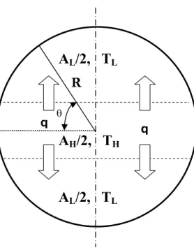
The Earth may be viewed as a closed system having two surfaces, a hot surface of area AH and temperature TH, which is heated by the Sun, and a cold surface (AL, TL) cooled by radiation to the

considered independent of longitude. The surface temperature is taken as its climatologic value, and represented by two temperatures (TH, TL) that correspond to the equatorial, and polar zones (AH, AL), the net collector and the net radiator, respectively (Fig. 1). The total heat transfer surface is fixed:

AH+AL=A (1)

The equatorial surface receives the solar heat current: 4 s p H sH A (1 )f T q = − α σ (2)

and radiates into space the heat current

4 H H

H A (1 ) T

q = − γ σ (3)

In eqs. (2) and (3) Ts, σ, f and α are the temperature of the sun as a black-body (5762K), the Stefan-Boltzmann constant (5.67 × 10–8 _{W m}–2_K–4_{), the Earth-sun view factor (2.16 × 10}–5_{), the} albedo of the Earth (0.35) and γ = 0.4 is the Earth's greenhouse factor, or the reflectance in the infrared region, respectively. The area AHp represents the projection of the area AH on a plane perpendicular to the sunrays and varies with the latitude θ as

θ π θ θ + θ = sin 2 cos sin A / A_{Hp H} (4)

The difference between qsH and qH is convected over the Earth’s surface, from AH to AL H

SH q

q

q = − (5)

In a similar way , the radiative balance of the net radiator is given by L

SL q

q

q+ = (6)

where qSL and qL represent the solar radiation absorbed and the heat radiated by the cold surface respectively, which are given by

4 s Lp L s A (1 )f T q = − α σ (7) and 4 L L L A (1 ) T q = − γ σ (8)

In Eqs. (3) and (8) the temperature of the background, T_∞4~3K, has been neglected because of its small value, as compared with TL and TH and α and γ are assumed to have the same values in both zones. From Eqs. (1)-(8) and with x = AH/A= sinθ, we obtain the heat balance of the net collector as (see also, [6]) 0 ) 1 ( R 4 / q T x ) x 1 ( x x arcsin B_ + − 2 1/2_ − _H4 − _ π 2σ − γ _ = (9)

In a similar way the heat balance of the net radiator is given by

0 ) 1 ( R 4 / q T ) x 1 ( ) x 1 ( x x arcsin 2 / B 2 1/2 _L4 2 =     _{π σ − γ} + − −    _{π − − −} (10) where 4 9 4 s ₂f 1₁ 4.1 10 K T B ≅ × γ − α − π = ₍₁₁₎

The fraction of the Earth’s surface area x, allocated to the net colector is unknown. There is a continuous set of partitions, x, of the Earth’s surface, which are solutions of Eqs. (9) and (10). However, the Constructal Principle indicates that the area actually allocated to the collector is the one that maximizes the heat current, q, flowing towards the radiator. In this case, the Constructal Principle is expressed by the simple mathematical expressions [6]:

0 x T , 0 x T , 0 x q 2L 2 L TH > ∂ ∂ = ∂ ∂ =       ∂ ∂ (12)

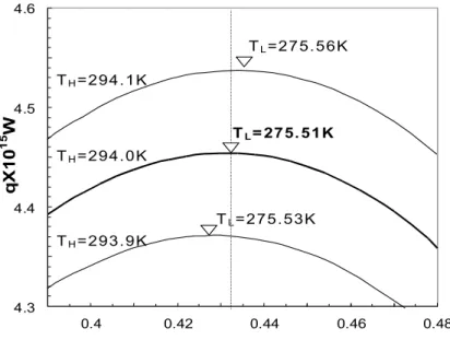
which imply that maximum heat current is achieved when the temperature of the radiator has the minimum value compatible with the heat balance equation (9). In order to apply these conditions to the global system we fix the temperature TH of the equatorial zone (the net collector) thus giving rise to the family of curves q(x)_{TH. To each T}H corresponds a curve with a well-defined maximum (e.g. qmax and xopt in Fig. 2, and to each maximum corresponds a temperature TL that is determined by combining Eqs. (9) and (10) in the form

B 2 T ) x 1 ( T x _H4 + − _L4 = π (13)

According to the Constructal Principle as defined by Eq. (12) the maximum heat flow corresponds to the minimum of TL, and this happens for TL=275.5 K, which enables the determination of the point of optimum performance as x = 0.434, TH=294.0 K and TL = 275.5 K (see, Fig 2).

In a way similar to that lead to Eq. (12), Constructal Principle determines the conditions of optimum performance of the heat sink as [6]

0 x T , 0 x T , 0 x q 2H 2 H TL < ∂ ∂ = ∂ ∂ =       ∂ ∂ ₍₁₄₎

Eq. (14) means that for maximum heat flow entering the net radiator (heat sink) the temperature of the hot zone (heat source) must have the highest value allowed by the energy balance defined by Eqs. (9) and (10).

In order to find the optimum performance point (TH, TL, x) we fix TL in Eq. (10), determine the points (qmax, xopt), and then locate the maximal TH, as required by the second and third conditions in

Eq. (14). Optimal performance of the net radiator (heat sink) is achieved for x = 0.8, TH = 288 K and TL = 265.5 K as shown in Fig. 3.

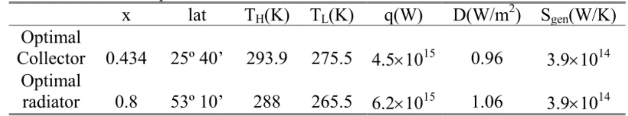
The latitude corresponding to the partition x=0.434 that determines the optimal performance of the net collector is 25°40' while 53°10' is the latitude that corresponds to the partition x=0.8 that defines the optimal performance of the net radiator. Figs. (4) and (5) show the results of both the optimization processes.

The optimal collector is the equatorial zone of average temperature TH = 294.0 K, which is located between 25°40' N and 25°40' S and the non-optimized net radiator is the ensemble of two surfaces of average temperature TL = 275.7 K, which are located above the latitude 25°40'.

The optimal radiator is the pair of polar caps above 53°10', with the temperature TL = 265.5 K, and the non-optimized heat collector is the equatorial zone of temperature TH = 288 K. The two zones between the latitudes 25°40' and 53°10', north and south, contribute to the average temperature of the non-optimized collector and to the average temperature of the non-optimized radiator. In this way, the average temperature of this zone THL may be evaluated as

0.434 × 294.0 K + (0.8 – 0.434)THL = 0.8 × 288 K (15)

and its value is THL = 281.5 K.

Both the optimization of the collector and of the radiator gives the same value for the Earth’s averaged surface temperature, which is 283.5 K. This temperature is determined in one and the other cases (x = 0.434, TH = 294.0 K, TL = 275.5 K) and (x = 0.8, TH = 288 K, TL = 265.5 K) as

<T>I = 0.434 × 294.0 K + (1 – 0.434) × 275.5 = 283.5 K (16)

and

The latitude 25°40' matches to the boundary between the Hadley cells and the Ferrel cells in both hemispheres and the latitude 53°10' approaches the latitude 60°, which is usually accepted to define the boundary between the Ferrel cells and the Polar cells.

We believe that the equator to pole temperature difference plays the major role in the definition of the three-cell regime of meridional circulation in line with the results of Stenzel and von Storch [9]. At slow rotation, the role of Earths’ rotation rate is determinant because it reduces the temperature gradient between dark and illuminated hemispheres, but for values of day rotation periods lower that 24 h it does not affect significantly the position of the three cells, as shown by Jenkins [8].

Additionally, the results of this optimization find further experimental support as they provide values for the convective conductance on the horizontal direction along the meridian (D) that may be calculated in both cases as [10]

) T T ( R π 2 q ~ D L H 2 ₋ (18)

where q is the heat flow corresponding to the optimal performances of the collector and of the radiator, respectively, and TH and TL are the corresponding temperatures. The values of D that match the optimal performances of the collector and of the radiator are 0.96 W/m2 and 1.06 W/m2, respectively, and fall in the range 0.6-1.1 W/(m2K) of the empirically evaluated values of D [10].

The total entropy generated on the Earth’s surface may be calculated as

      ₋ +       ₊ − ₋ − = H L s L H 2 0 gen S (1 α)πR _Tx (1_T x) _T1 q _T1 _T1 S (19)

where the solar constant S0 = 1380 W/m2 is the solar radiation (power per unit area perpendicular to the sun rays), α is the albedo of the Earth, and Ts = 5762 K is the sun temperature. Fig. 6 shows the

entropy generation on Earth’s surface for the case of optimal collector and for the case of optimal radiator together and Table 1 shows a synopsis of the main results of the optimization process.

Table 1. Values of several variables that match the cases of optimal collector

and optimal radiator.

x lat TH(K) TL(K) q(W) D(W/m2) Sgen(W/K)

Optimal

Collector 0.434 25º 40’ 293.9 275.5 4.5×1015 _{0.96 3.9×10}14

Optimal

radiator 0.8 53º 10’ 288 265.5 6.2×1015 _{1.06 3.9×10}14

One of the two maxima of entropy generation occurs when the partition of the Earth’s surface corresponds to the optimal collector while the other maximum occurs for a partition very close to that corresponding to the optimal radiator.

The first maximum matches the latitude of the boundary of the Hadley and Ferrel cells while the second one falls somewhat above to the boundary between the Ferrel and the Polar cells. As shown in Fig. 6, the entropy generation corresponding to each of Earth’s optimal partitions (x=0.434, x=0.8) has practically the same value 3.9×1014 _W/K.

We note that neither TH and TL nor the Earth’s surface partitions were assumed in advance. As it is usual with Constructal theory they came out of the optimisation process.

1.3 Latitudinal heat transport by vertical loops

The latitudinal temperature differences are the exergy source that powers the Earth’s meridional circulations. The available exergy is converted into potential energy with the help of gravity, trough buoyancy forces, and then into kinetic energy that is dissipated by the friction forces, which act as the brake of the flow, namely in the Earth’s boundary layer. Therefore vertical loops develop for meridional heat transport from the equatorial belt to the polar caps. The pressure difference that drives the boundary layer flow is given by [6]

(

)

(

)

P

∆ _L − _{H H} − _L (20)

It is opposed and balanced by the shear force thereby maintaining an average flow velocity given by

2 / 1 2 L H L H ) T T ( ξ g β 10 ~ v _      − (21)

Here, ρ, g, H and L represent density, acceleration due to gravity, height of the boundary layer and distance between the two branches of the counterflow, respectively, β the coefficient of volumetric thermal expansion and ξ = (1– βgH/Rg)–1 a factor that results from the expansion and linear approximation of ρ = P/(RgT), namely, ρL – ρH = βρ(TH – TL) + kTρ(PL – PH), where kT is the isothermal compressibility, kT =ρ–1(∂ρ/∂P)T.

The total heat flow transported by each vertical loop, which is supposed to develop symmetrically with respect to Earth’s rotation axis, is given by [6]

2 / 3 L H 2 / 3 (T T ) C q= − (22)

Here C3/2 is a new kind of heat conductivity proposed by A. Bejan [6] that is given by

σ ) γ 1 ( R π 4 ) x ( W ) x ( L H ) βξ g ( ) R / c ( ρ 12 C ₂ 2 / 1 3 2 / 3 g p 2 / 3 − = − (23)

where R is the radius of the Earth, L(x) and W(x) are known geometric functions of the fraction x of the Earth’s surface allocated to the collector, which represent the length of the loop boundary layer along the meridian and the width of the loop along the parallel, respectively.

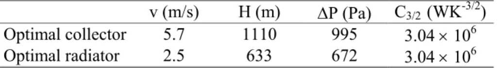
This huge loop is supposed to transport all the heat from the optimal net collector to the radiator. This heat flow is the input variable to Eqs. (20)-(23), which allow for the calculation of the average pressure difference between the two branches of the counterflow ∆P, the average latitudinal velocity v, and the C3/2 conductivity. These results and values of the variables corresponding to the optimal net radiator, which were calculated in an analogous way are shown in Table 2.

Table 2. Average velocity of the latitudinal flow, heigh of the boundary layer,

pressure difference between the branches of the counterflow at Earth’s surface, and C3/2 conductivity, for optimal collector and optimal radiator

v (m/s) H (m) ∆P (Pa) C3/2 (WK-3/2)

Optimal collector 5.7 1110 995 3.04 × 106

Optimal radiator 2.5 633 672 3.04 × 106

The values of v, H, and ∆P, in Table 2 scale with the observed values of the meridional circulation. The average latitudinal velocity and the height of the friction layer are higher at the latitude 25°40' than at the latitude 53°10', which is in fair agreement with the observed wind intensity relation between the Ferrel westerlies at each of these latitudes. The average latitudinal component of these winds points northward, starts in the vicinity of latitude of 30° and reaches a maximum at the latitude 53° [11, p. 128].

The average pressure in the equatorial zone is PH ~ (PE + Pθ)/2, and in the polar caps is PL ~ (Pθ + PP)/2, where PE, PP and Pθ stand for the pressure at the equator, at the pole and at the boundary between the two zones, respectively. By noting that ∆P =PH – PL = (PE – PP)/2, we find that the pressure differences between the two zones presented on Table 2 (i.e. 995 Pa and 672 Pa) give for (PE – PP)=2<∆P>~1667 Pa, which agrees in a scaling sense with the observed average mean sea-level pressure difference between the equator and the poles (PE – PP) that is of order of 1500 Pa.

However the most intriguing feature is that the C3/2 conductivity has exactly the same value in both cases. This conductivity comes out of the model of vertical convection loops. We may speculate that the optimisation of heat transfer on Earth’s surface implies vertical circulation loops as the heat transport mechanism.

3. Maximization of heat transfer performance at daily scale

We analyse here the heat transfer between illuminated and dark hemispheres of Earth. The collector area corresponds to the illuminated part of the Earth surface, and the radiator corresponds to the dark part. As the sun rays are practically parallel the collector area, the illuminated area is half of the Earth surface (x=AH/AL≅1/2). The excess heat in the illuminated hemisphere, the collector, is transported by the Earth's rotation (note that the boundary between the illuminated and the dark hemisphere is moving as the Earth rotates), while the rest is convected over the Earth surface (see Fig. 7).

The Earth’s rotation transfers heat continuously from the illuminated hemisphere to the dark hemisphere even in the absence of convection, as the boundary between the illuminated and dark surfaces moves with a speed equal to the Earth rotation speed at the same latitude. A relatively small part is convected at the average velocity u, from the illuminated to the dark surface. Because the collector area is equal to the radiator area, the parameter that is allowed to vary in the constructal optimization of the flow configuration is the average velocity of the atmospheric air relative to the Earth surface.

The heat flow from the collector at temperature TH to the radiator at temperature TL is given by:

(

)

[

(

)

]

q_d = _{H p H} − _{L p L 0} + (24)

Here U0 = 462 ms–1 is the Earth rotation velocity at the equator, 2U0/π., is the rotation velocity averaged over the meridian, H is the height of the friction layer, u is the average convection velocity of the planetary fluid relative to the Earth surface (Fig. 7), and Λ ~ 1.2 represents the mean ratio of total enthalpy to sensible heat in the air.

(

)

which may be related to the total power dissipated by fluid friction on the Earth surface, wd = (PH – PL) u2πRH, as       ₊ = 1 u π U R c Λ w q 0 g p d d (26)

The heat qd that flows to the cold region and afterwards is radiated into space, may also be written as 4 L 2 d 2πR (1 γ)σT q = − (27)

We note that that Eq. (26) represents the sum of two heat currents: the current that is transported to the radiator by the Earth rotation in the absence of fluid flow relative to the Earth surface, that is

u π U R c Λ w q 0 g p d 0 d = (28)

and the current qdc convected by the fluid motion relative to the Earth surface

g p d c d _R c Λ w q = (29)

The Constructal Principle requires the fluid flow structure to develop on the purpose of maximizing the heat current qdc convected from the collector to the radiator. Because the partitioning of the Earth surface is fixed (x = 1/2), the optimization is made with reference to the other free parameters of the flow structure: the velocity u and the height of the friction layer, H. Then, we combine u and H into a non-dimensional group, the Ekman number (Ek), with respect to which the convective heat current can be maximized.

In view of the fact that U/u >> 1, again with the help of the ideal gas law, P=ρRgT, from eqs. (26) and (27) we obtain Ek ε C T_L4 ≅ ₀ d (30)

where εd is a power density,

u ) P P ( ) RH π 2 /( w ε_d = _d = _H − _L (31)

and C₀ = Λc_p /

(

)

H u 2 u C Ek 2 D ω = (32)

Here CD ~ 0.01 represents the friction coefficient in the boundary layer [12]. The Ekman number represents the ratio of the friction forces CDρu2/H to the Coriolis forces 2ρωu.

Since AH = AL, or x = 1/2, the overall radiative balance given by Eq. (13) is now modified to B T T 4 H 4 L+ =π (33)

The average convective velocity u is given by Eq. (21), which together with Eqs. (30)-(33) becomes 2 2 D 2 2 0 1 2 1 L H R g β ξ C π 100 L U 16 C , Ek C T T = + = (34)

Here C1 is a constant, ξ has the same meaning as in Eq. (21), and the brackets indicate average values in the interval [TL,TH]. Therefore, by combining the Eqs. (33), (34) and (30) we obtain

B π Ek ε C Ek C Ek ε C ₀ d 4 2 1 4 / 1 d 0 + =         +       (35)

This equation expresses the power density εd as function of the Ekman number as shown in Fig. 8. From the curve εd (Ek) and Eqs. (30) and (34) we determine TL and then TH. Next, Eqs. (31) and (32) together with Eq. (20) enable us to calculate the height of the friction layer as

(

)

In the calculations leading to Eq. (36) we took L/<ξ> ~ 1.2 R, which results from L = π1/2_{R. The} average velocity u follows from Eq. (32). From Eqs. (29) and (31) we determine the convective heat current qdc(Ek) that is shown in Fig. 9, and has a maximum at Ek=0.2.

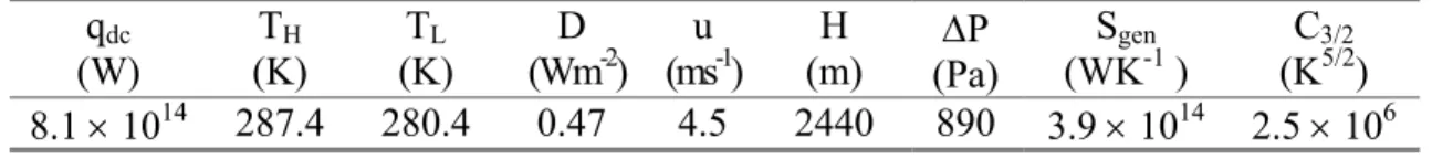
The curves corresponding to the average convective velocity, temperatures, height of the boundary layer and pressure difference, which was determined from Eq. (31), are shown in Fig. 10. Table 3 shows a synopsis of all results, including the overall entropy generation on Earth and the C3/2 conductivity, which were calculated from Eqs. (19) and (22), respectively.

Table 3 Flow variables that result from optimisation of heat transfer between illumiated and dark hemispheres

qdc (W) TH (K) TL (K) D (Wm-2) u (ms-1) H (m) (Pa) ∆P Sgen (WK-1 ) C3/2 (K5/2) 8.1 × 1014 _{287.4 280.4 0.47 4.5 2440 890 3.9 × 10}14 _{2.5 × 10}6

These predictions may be refereed against observational values. The main important aspects are: 1. The average temperature difference TH – TL between day and night is 7 K. This agrees in order of magnitude with the average diurnal amplitudes observed on Earth, which for the maritime areas is around 3 K and for continental areas is around 10 K ([11], p. 44).

2. The average temperature of the Earth’s surface is (TH+TL)/2~283.9 K, which is almost the same value that results from the optimization of the latitudinal heat transport.

3. The entropy generation rate calculated on the diurnal scale has the same value as that found from the optimization of the latitudinal heat transport in spite of the variables used in these two Sgen calculations being derived in very different ways. For the latitudinal heat transport, the heat current was determined as function of the Earth partition x, while for the diurnal scale it was determined as function of the Ekman number which involves the Earth rotation velocity, the height of the friction layer and the fluid flow velocity.

4. Even though the temperatures (TH, TL) and the heat current at daily scale differ from those corresponding to latitudinal heat transport the variables defining the properties of the friction layer have values of the same order of magnitude.

5. Dai and Wang [13] used pressure data of the period 1976-97 from meteorological stations covering the Earth’s surface and found that diurnal tides between dark and illuminated hemisphere exist in global surface pressure fields, with amplitudes of order 2 mb. The theoretical results shown in Table 3 predict amplitudes of order 890 Pa ~9 mb. Even though the prediction did not match the observed values, it is of same order.

6. The average heat flow between the illuminated and dark hemispheres (qdc) is roughly 6 or 7 times lower than the poleward current. However, the convective conductance in the horizontal direction (D) and the conductivity (C3/2) both have values of the same magnitude as those obtained for the latitudinal transport.

Another interesting remark comes from the analysis of the TH and TL curves in Eq. (10). The value of the Ekman number as well as those of all other variables in Table 3, came out of the optimisation of the heat flow. Two of these variables, the average velocity u, and the height of the boundary layer H, enter in the definition of Ek (see, Eq. (32)). The third variable is the angular speed of rotation of the Earth, which is an input variable to the model. It is known that the Earth rotation is continuously being slowed down due to ocean tidal friction therefore making the length of the day longer and longer by about 15 seconds per million years. At this rate the speed of rotation

will decrease 15% one billion years from now and the optimal Ekman number will go up to 0.23. Therefore the diurnal amplitude of temperature will increase up to 10 K and the Earth’s climate will be rather different from now. This is another varying parameter determining climate changes on Earth.

2. From Constructal theory to actual river basins

Flow architectures are ubiquitous in Nature. From the planetary circulations to the smallest scales we can observe panoply of motions that exhibit organized flow architectures: general atmospheric circulations, oceanic currents, eddies at the synoptic scale, river drainage basins, dendritic crystals, etc. Fluids circulate in all living structures, which exhibit special flow structures such as lungs, kidneys, arteries and veins in animals, and roots, stems, leaves in plants.

Rivers are large scale natural flows that play a major role in the shaping of the Earth’s surface. River morphology exhibits similarities that are documented extensively in geophysics treatises. For example, Rosa [14] in a recent review article gives a broad list of allometric and scaling laws involving the geometric parameters of the river channels and of the river basins.

In living structures heat and mass flows occur for the same reason, i.e. dissipating minimum exergy they reduce the food or fuel requirement, and make all such systems (animals, and “man + machine” species) more “fit”, i.e., better survivors.

Constructal theory views the naturally occurring flow structures (their geometric form) as the end result of a process of area to point flow access optimisation with the objective of providing minimal resistance to flow (see Bejan, [4]).

Natural systems are complex and change in many ways. In the past, scientists realized that for understanding nature they had to focus their attention on simple and homogenous systems. Motion, as the change of relative position with time, is the ubiquitous phenomenon that called for explanation, and the principle of least action is the principle that unified motions from point to point

in a common picture. The constructal law is its counterpart, by allowing systems with complex internal flows to be described and understood under a unified view.

2.1 Scaling laws of river basins

River basins are examples of area to point flows. Water is collected from an area and conducted trough a network of channels of increasing width down to the river mouth. River networks have long been recognized as being self-similar structures over a range of scales. In general, small streams are tributaries of the next bigger stream in such a way that flow architecture develops from the lowest scale to the highest scale, ω (see Fig. 11).

The scaling properties of river networks are summarized in well-known laws. If Li denotes the average of the length of the streams of order i, Horton’s law of stream lengths [14, 15-17] is

L 1 i

i L R

L ₋ = ₍₃₇₎

where RL is Horton’s ratio of channel lengths, while Horton’s law of stream numbers [14, 15-17] is B

i 1

i n R

n ₋ = ₍₃₈₎

where ni is the number of tributaries of a stream of order i, and RB is Horton’s bifurcation ratio. In river basins RL ranges between 1.5 and 3.5, and is typically 2, while RB ranges between 3 and 5, typically 4, [15].

The mainstream length Lω and the area Aω of a river basin with streams up to order ω, are related trough Hack’s law [14, 15, 18, 19]:

Lω = α(Αω)β (39)

where α ~ 1.4 and β ~ 0.568 are constants [19].

If we define a drainage density Dω = LT/A where LT is the total length of streams of all orders and A the total drainage area and a stream frequency Fs= Ns/A, where Ns is the number of streams of all orders, then Melton’s law [14, 16, 20] indicates that the following relation holds:

(

)

F = ₍₄₀₎

Other scaling laws relate discharge rate with river width, depth, and slope (see Rosa, [14]).

2. 2 River networks as constructal fluid trees.

River basins are examples of area-to-point flow, which is a classical topic of constructal theory. Adrian Bejan has addressed this type of flows and optimized the channel network that minimizes the overall resistance to flow. A detailed treatment can be found one of his books [4]. Here we summarize the optimized area-to-point flow geometry when the permeability of a channel of width D is given by K= (1/12)D2 , which corresponds to Hagen-Poiseuille flow between parallel plates. Therefore, if Hi and Li represent the dimensions of the area allocated to each stream of order i (see Fig. 12) and ni is the number of streams of order i that are tributaries of each stream of order i+1, then the optimized values are shown in Table 4.

Table 4 - The optimised geometry of area-to-point flow (channels with Hagen-Poiseuille flow, (Bejan, [4]) (Kˆ=K/A₀; (H~_i,~L_i)=(H_i,L_i)/(A₀)1/2; Φ_i =D_i /H_i). Order H~_i L~_i ni 0 2 / 1 0 6 / 1 6 / 1 6 / 5 Φ Kˆ 3 2 6 / 1 6 / 1 6 / 5 2 / 1 0 Kˆ 3 2 Φ - 1 6 / 1 6 / 1 2 / 1 0 6 / 1 Kˆ 3 Φ 2 2 / 1 2 / 3 2 / 3 1 Kˆ 2 Φ 3 / 2 6 / 1 3 / 4 2 / 1 0 2 / 3 1 Kˆ 3 2 Φ Φ 2 2 / 1 2 / 1 2 / 3 1 Kˆ 2 Φ 6 / 5 2 / 1 0 3 / 5 2 / 3 1 2 6 / 1 Kˆ Φ 2 ) Φ Φ ( 3 3 / 2 0 6 / 5 2 / 3 2 3 / 1 Kˆ Φ 2 ) Φ Φ ( 3 3 6 / 5 2 / 1 0 3 / 2 2 / 3 1 2 6 / 1 Kˆ Φ 2 ) Φ Φ ( 3 6 / 7 0 3 / 4 2 / 3 1 2 3 3 / 1 Kˆ Φ 2 ) Φ Φ Φ ( 3 3 / 2 0 2 / 3 2 3 3 / 1 6 / 1 Kˆ Φ ) Φ Φ ( 3 2 4 6 / 7 0 3 / 1 2 / 3 1 2 3 3 / 2 Kˆ Φ 2 ) Φ Φ Φ ( 3 6 / 9 2 / 3 0 2 / 1 2 / 3 1 2 3 4 2 / 1 Kˆ Φ 2 ) Φ Φ Φ Φ ( 3 3 / 2 0 2 / 3 3 4 3 / 2 6 / 7 Kˆ Φ ) Φ Φ ( 3 2

The void-allocation (channel) optimisation provides the additional relationships [4]:

0 1 Φ

Φ = ; Φ₂ =

(

)

(

)

(

)

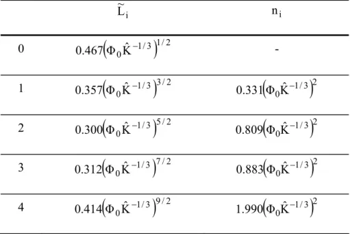
Table 5. - The jointly optimised network parameters (minimization of the overall resistance to flow and optimisation of void (stream area) allocation)

i L ~ i n 0

(

)

(

)

(

)

(

)

(

)

(

)

(

)

(

)

(

)

Both L~_iand n_i depend uniquely on Φ₀Kˆ−1/3which in turn is the product of two terms: (i) Φ that ₀ represents the ratio of the area of the smallest (first order) channel to the area of the porous layer that feeds it and (ii) the dimensionless permeability Kˆ raised to the power (–1/3).

As none of these parameters depend upon the particular geometry of the layer we conclude that despite the relationships of Tables 4 and 5 were derived from constructs of regular geometry as that of Fig. 12, the relationships in Table 5 are applicable to any hierarchized stream network irrespectively to its particular geometry. Channel hierarchy is understood in the Hortonian sense, i.e. all streams of order i are tributaries of streams of order i+1.

River basins are examples of area-to-point flows that approach the Hortonian hierarchy, therefore the constructal rules defined in Table 5 for stream networks up to order 4 must hold, at

least approximately. For example, with the use of Table 5, the ratios of the lengths of consecutive streams are given in Table 6.

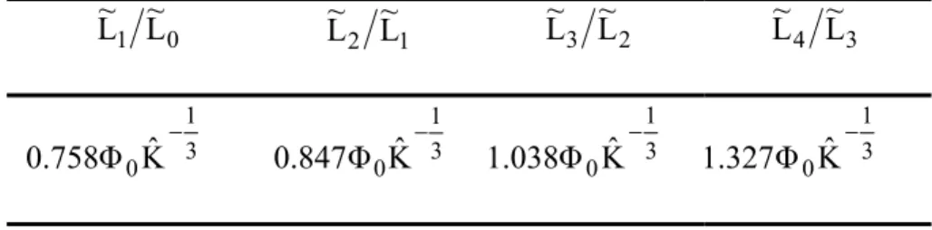
Table 6 - Constructal Horton ratios of stream lengths, RL.

0 1 L~ L~ L~₂ L~₁ L~₃ L~₂ L~₄ L~₃ 3 1 0Kˆ Φ 758 . 0 − 3 1 0Kˆ Φ 847 . 0 − 3 1 0Kˆ Φ 038 . 1 − 3 1 0Kˆ Φ 327 . 1 −

We see that the ratio of the characteristic lengths of streams of consecutive order

3 / 1 0 i 1 i L~ ~Φ Kˆ L ~ −

− is practically constant as required by Horton’s law of stream lengths (Eq. 37).

To check if the constructal relations in Table 5 match Horton’s law of stream numbers (Eq. 38) we calculate the number Ni of streams pertaining to order i, which is given by:

1 2 i 1 i i i n n n ... n N = × ₋ × ₋ × × (42)

where nj is the number of streams of order j that are tributaries of each stream of order j+1. Taking into account Eq. (42), the ratio of the number of streams of order i-1 to the number of streams of order i is given by:

i 1 i

i N n

N ₊ = (43)

which is the number of streams ni of order i already shown in table 5. We conclude that these ratios are almost of the same order, i.e. N_i N_i+1 ~

(

)

(

)

i.e., the ratio of stream numbers is of the order of the square of the ratio of stream lengths. As stated in the introduction, in real river basins Lι/Lι−1 = RL ranges between 1.5 and 3.5, and is typically 2, while Nω-1/Nω = RB ranges between 3 and 5, typically 4 [14, 15, 17], i.e. the constructal rule evinced by Eq. (44) is closely verified for the real river basins.

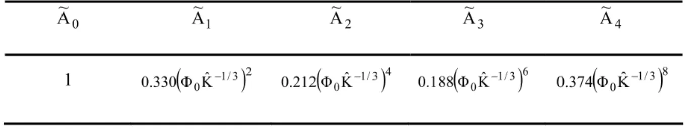
Next we will show that Hack’s law, (Eq. 39) also follows from the constructal relationships of Tables 4 and 5. Noting that A_i =H_iL_i and using Table 4 and Eqs. (41) we obtain the sub-basin areas shown in Table 7.

Table 7 – Dimensionless area of constructal river basins up to order 4 0 A~ A~₁ A~₂ A~₃ A~₄ 1

(

)

(

)

(

)

(

)

The constructal relationship between the mainstream length Lω and the area Aω of a river basin with streams up to order ω is determined by using this table together with Table 5, and is shown in Table 8.

Table 8 – Constructal Hack’s exponent β for river basins up to order 4. 750 . 0 1 1 ~A L~ L~₂ ~A0₂.625 ~L3 ~A30.583 L~4 ~A04.563

Gray [21] found β ~ 0.568 while Muller [22] reported that β ~ 0.6 for river basins less than 8000 mi2_{, β ~ 0.5 for basins between 8000 and 100,000 mi}2 _{and β ~ 0.47 for basins larger than 100,000} mi2 (see also [19]).

ω 4 1 ω 2 β_ω = + (45)

We see from Eq. (45) that as the order of the river basin increases, β approaches 0.5 in good agreement with Muller’s findings for actual river basins.

In order to check Melton’s law, first we calculate the drainage density Dω as: ω ω ω 1 i i i ω n L~ H~ L~ D = ∑ = (46)

and the stream frequency as

ω L ~ H~ N F ω _ω 1 i i ω =∑ = (47)

By using Tables 1 and 2 and with the help of Eq. (42) we obtain:

(

)

(

)

(

)

(

)

(

)

(

)

(

)

We note that the drainage density of a stream of order 0 is (L₀ H₀)1/2while the stream frequency is 1, which is its lowest limit.

(

)

0Kˆ

Φ 374 .

0 −

The variation of F4 with D4 is shown in Fig. 13. We see that the constructal relations (48) and (49) follow Melton’s law quite approximately in the range 1 < D4 < 100, i.e. F4 is proportional to D4 raised to the power 2.45.

In accordance with the Constructal Law, the scaling laws of river basins evince the organized flow architectures that result from the underlying struggle for better performance, by reducing the overall resistance in order to drain water from the basins the fastest.

Constructal theory views the naturally occurring flow structures (its geometric form) as the end result of a process of area to point flow access optimisation with the objective of providing minimal resistance to flow. For example, the features of the river drainage basins can be anticipated based on the area-to-point flow access optimization presented in section 2. The generation of dendrite-like patterns of low resistance channels can be understood based on a simple model of surface erosion together with a principle that is invoked at every step. The model assumes that the changes in the river channel are possible because finite blocks can be dislodged and entrained in the stream. As a rule (principle), every squared block of area L2 and height W, is dislodged whenever the pressure difference ∆P across the block surpasses the critical force needed to dislodge it, i.e. ∆PLW > τL2_, ([4], [14]). The flow resistance decreases with block removal. Further increase in the flow rate may create the conditions for the removal a second block and for the repetition of the process. A macroscopic dendrite-like structure emerges progressively (see Fig. 14) while flow resistance decreases.

Other impressive features of river morphology are the sinusoidal shape of river channels, which wavelength (λ) is proportional to the channel width (λ ~W) that, in turn, is proportional to the maximum depth, w ~ d. Constructal theory links geometry to performance of river flow and explains how this geometric relations result from the minimization of global resistances (Bejan [4]. The bottoms of river channels are round or nearly round. The same occurs in living structures (blood vessels, pulmonary airways, etc.). Calculations show that the flow resistances decrease as the shape becomes rounder. Although the round shape is the best, the nearly round shapes perform almost as well ([4], [24]).

The Constructal law, (Bejan [4]), states that if a system has freedom to morph it develops in time the flow architecture that provides easier access to the currents that flow trough it. In all classes of flow systems (animate, inanimate, engineered) the generation of flow architecture emerges as a universal phenomenon. According to Constructal theory the optimal structure is constructed by optimizing volume shape at every length scale, in a hierarchical sequence that begins with the smallest building block and proceeds towards larger building blocks (which are called “constructs”). A basic outcome of Constructal theory is that system shape and internal flow architecture do not develop by chance, but result from the permanent struggle for better performance and therefore must evolve in time [25].

Bejan used Constructal theory to successfully explain some allometric laws of living structures namely the rhythm of respiration in animals in relation with body size [27], the relation between metabolic rate and total body volume [4, 26], and the heartbeat frequency in relation to metabolic rate [4, 27]. Reis et al. [28] focused on the structure of the pulmonary airflow tree, which starts at the trachea and bifurcates 23 times before reaching the alveolar sacs. Until now, the reason for the existence of just 23 bifurcations in the respiratory tree has remained unexplained in the literature. Has this special flow architecture been developed by chance or does it represent the optimum structure for the lung’s purpose, which is the oxygenation of the blood?

3.1 Purpose of the lungs and trade-off between competing trends

Even though every living fluid tree works with a specific purpose, all share some general features. For example, every living fluid tree works either for the delivery of substances to a volume or a surface where a process occurs, e.g. a chemical reaction, or for the removal of other substances including the products of chemical reactions. At the smallest scale diffusion dominates while channelling of the flow and development of flow architectures occur at higher scales. Fig. 12 illustrates how a first channel of width D0 and conductivity K0,collects the fluid that permeates the

rectangular area and delivers it to a wider channel (D1, K1). Channels organize hierarchally in a flow architecture in which channels of lower conductivity are tributaries of a channel of higher conductivity.

As illustrated in Fig. 12, increase in the number of the elementary areas through which fluid diffuses implies increasing number of channels, and therefore increasing resistance to fluid flow. On the other hand, if the number of channels is reduced, the resistance to fluid flow is also reduced accordingly but in this case, the elemental rectangle has to have a larger area, therefore increasing the resistance to fluid diffusion. The optimal flow architecture is the one that results from the trade-off between these two competing trends.

In line with Bejan’s Constructal law, we believe that every living system has developed in time the flow architecture that provides easier access to the currents that flow trough it. As a leading example of a living flow structure, we focus on the human respiratory tree. By using Constructal theory, Reis et al. [28] addressed the study of the respiratory tree as a flow system with duct flow resistances (trachea and bronchial system) and diffusive resistances. In their study, to evaluate and compare the flow resistances, was considered that oxygen and carbon dioxide flow within the respiratory tree (bronchial tree plus alveolar sacs) as driven by the chemical potential. This is a rather convenient potential because pressure differences that drive the isothermal airflow in the bronchial system may be expressed in terms of chemical potential differences trough the generalized Gibbs-Duhem equation, ∆µ=ρ−1∆P+∆ε, where ε stands for kinetic energy per unit mass (see [28] for details). The bronchial tree was assumed to be composed of cylindrical channels with Hagen-Poiseuille flow. Even though the bronchial channels are not perfectly round, Bejan has shown that nearly round channels perform almost as well as the exactly round channels [25].

For laminar flow, Constructal theory indicates that the minimum flow resistance at a bifurcation is achieved if the ratio between consecutive duct diameters is:

Dn/Dn-1 = 2-1/3 (50) while the ratio of the respective lengths, is

Ln/Ln-1 = 2-1/3 (51) These relations that are theoretically predicted by Constructal theory were discovered empirically long ago and correspond to the so-called Murray’s laws.

After having considered every detail of the flow between the entrance of the trachea and the alveolar surface where oxygen meets the blood and carbon dioxide is removed from the blood, including the resistances due to bifurcations, Reis et al. [28] showed that the global resistance (J s kg-2 ) to oxygen transportation within the respiratory tree is of the form,

(

)

[

]

( )

In Eq. (52), N matches to the number of bifurcations of the bronchial tree, ν is the kinematic viscosity of the air, L0 and D0 represent trachea length and diameter, respectively, T is temperature, φox and (φox)0 represent the relative concentration of oxygen in the alveoli and in the outside air, respectively, Dox is the diffusivity of the oxygen in the air, Rg is the air constant and ρ stands for the density of the air.

The first term in the r.h.s. of Eq. (52) represents the global channel flow resistance (bronchiolar tree) while the second term matches to the global diffusive resistance to oxygen transport in the alveoli. Equation (52) with the corresponding variables holds also for the resistance to carbon dioxide flow in the respiratory tree. These resistances can be evaluated by assuming a body temperature of 36ºC and taking al pertinent values at this temperature. The average value of oxygen relative concentration within the respiratory tree, φox, may be evaluated from the alveolar air equation in the form: ((φox)0-φox)Q-S=0, where (φox)0 ~1/2(φair+φox) and φair are the oxygen relative

airflow and S is the rate of oxygen consumption. With (φox)air=0.2095, Q~6×10-3 m3/min and S~0.3×10-3 _m3_{/min we obtain φ}

ox ~ 0.1095. The value of the average relative concentration of carbon dioxide in the respiratory tree, φcd=0.04. In this case we used S=0.24×10-3 m3/min since the respiratory coefficient is close to 0.8 and (φcd)air ~ 0.315×10-3.Anatomic treatises [29, 30] indicate that L0 is typically 15 cm, while the trachea diameter, D0, is approximately 1.5 cm. The global resistances to oxygen and carbon dioxide transportation in the respiratory tree are plotted against number of bifurcations in Fig. 15.

The minimum of each resistance occurs close to N = 23. This same result can be obtained by finding the number of bifurcations Nop analytically that matches to the minimum of the global resistance (see Eq. (52)). This minimum is given by:

( )

(

)

With the same values used for the respective curves in Fig.16. we found Nop = 23.4 and Nop = 23.2 for the oxygen and the carbon dioxide transport, respectively. As the number of bifurcations must be an integer we conclude that it must be 23.

A first result is that the human respiratory tree that bifurcates 23 times between the trachea and the alveoli is optimized both for oxygen access and for carbon dioxide removal. The trade-off between resistance to flow in the bronchial tree and resistance to oxygen and carbon dioxide diffusion in the alveoli is achieved by the human respiratory tree, which has been optimized by nature in time. A second outcome is that the actual flow architecture of the respiratory tree can be anticipated theoretically based on Constructal theory.

We see from Eq. (53) that the number of bifurcations that matches to minimal global resistance to oxygen access an carbon dioxide removal is function of several environmental variables such as normal body temperature, oxygen and carbon dioxide diffusivities and concentrations in the air, air kinematic viscosity and only one morphological parameter, which is the length λ=D₀2 L₀ . As every individual lives with the same the average environmental parameters, we conclude that if the respiratory tree with 23 bifurcations is a characteristic of humankind therefore the number λ is also a characteristic of humankind. In other words, the ratio of the square of trachea diameter to its length is the same for every human being. This theoretical result is anticipated by Constructal theory and now awaits confirmation by the anatomists.

Another constructal relationship involving the length λ, the area allocated for the respiratory process (the total area of the alveoli) A, the volume of the lungs V, and the length of the respiratory tree (between the entrance of the trachea and the surface of the alveolus) L, was also derived by Reis et. al. [28] and is the following:

_{( )}

[

]

From Eq. (5) we conclude that the non-dimensional number AL/V, determines the characteristic length λ=D02/L0, which in turn determines the number of bifurcations of the respiratory tree by Eq. (53). This constructal relationship may be summarized as follows: “The alveolar area required for gas exchange A, the volume allocated to the respiratory system V, and the length of the respiratory tree L, which are constraints posed to the respiratory process determine univocally the structure of the lungs, namely the bifurcation level of the bronchial tree.” Here we may observe the realm of Constructal theory, which is minimization of global resistances to fluid access under geometric constraints imposed to the process.

References

[1] E. N. Lorenz, 1975, “Climate Predictability”, in The Physical Basis of Climate and Climate Modeling, World Meteorological Organization, Geneva, Switzerland, GARP, Vol. 16.

[2] J. P. Peixoto and A. H. Oort, 1992, Physics of Climate, American Institute of Physics, New York, pp. 520-1992 .

[3] G. A. Mehel, 1992, “Global Coupled Models: Atmosphere, ocean, sea ice”, in Climate System Modelling, Cambridge University Press, Cambridge, pp. 555-81,

[4] A. Bejan, 2000, Shape and Structure, from Engineering to Nature, Cambridge University Press, Cambridge, UK.

[5] A. Bejan and A. H. Reis, “Thermodynamic optimization of global circulation and climate”, to be published in Int . J. Energy Research.

[6] A. H. Reis and A. Bejan, “Constructal theory of global circulation and climate”, to be published. [7] A. Navarra and G. Boccaleti, 2002, “Numerical general circulation experiments of sensitivity to Earth rotation rate” Climate Dynamics, Vol. 19, pp. 467-483.

[8] G. S. Jenkins, 1996, “A sensitivity study of changes in Earth’s rotation rate with an atmospheric general circulation model”, Global and Planetary Change, Vol. 11, pp. 141-154.

[9] O. J. Stenzel and J. S. von Storch, 2004, “On the effect of thermal forcing on the global atmospheric angular momentum and the general circulation”, Climate Dynamics, Vol. 22, pp. 415-427.

[10] R. D. Lorenz, J. I. Lunine, C. P. McKay and P. G. Withers, 2001, “Titan, Mars and Earth: entropy production by latitudinal heat transport”, Geophysical Research Letters, Vol. 25, , pp. 415-418.

[11] R. G. Barry and R. J. Chorley, 1998, Atmosphere, Weather and Climate, 7th Ed., Rutledge, London and N. York.

[12] S. Pal Arya, 1988, Introduction to Micrometeorology, Academic Press, London.

[13] A. Dai and J. Wang, , 1999, “Diurnal and semidiurnal tides in surface pressure fields”, J. Atmospheric. Sciences, Vol. 56, pp. 3874 -3891.

[14] Rosa, R. 2004. “River basins: geomorphology and dynamics”, Bejan’s Constructal Theory of Shape and Structure, pp. 15-47, Edts. R. Rosa, A. H. Reis and A. F. Miguel, CGE, Évora,.

[15] Rodríguez-Iturbe, I and Rinaldo A. 1997. Fractal River Basins, Cambridge University Press, New York.

[16] Horton, R. E. 1932. “Drainage basin characteristics”, EOS Trans. AGU, Vol 13, pp. 350-361. [17] Raft, D. A., Smith, J. L. and Trlica, M. J. 2003. “Statistical descriptions of channel networks and their shapes on non-vegetated hillslopes in Kemmerer, Wyoming”, Hydrol. Process, Vol. 17, pp. 1887-1897.

[18] Hack, J.T., 1957. “Studies of longitudinal profiles in Virginia and Maryland”, USGS Professional Papers 294-B, pp. 46–97.

[19] Schuller, D. J., Rao, A. R. and Jeong, G. D. 2001.“Fractal characteristics of dense stream networks”, J. Hydrology, Vol. 243, pp. 1-16.

[20] Melton, M. A, 1958. “Correlation structure of morphometric properties of drainage systems and their controlling agents”, J. Geology, Vol. 66, pp. 35-56.

[21] Gray, D.M., 1961. “Interrelationship of watershed characteristics”, J. Geophysical Research, Vol. 66, pp. 1215–1223.

[22] Muller, J.E., 1973. “Re-evaluation of the relationship of master streams and drainage basins: reply” Geological Society of America Bulletin Vol. 84, 3127–3130.

[23] M. R. Errera and A. Bejan, "Deterministic Tree Networks for River Drainage Basins," Fractals, Vol. 6, No. 3, 1998, pp. 245-261

[24] A. Bejan and S. Lorente “The constructal law and the themodynamics of flow systems with configuration”, International Journal of Heat and Mass Transfer, Vol. 47, 2004, pp. 3203-3214.

[25] Bejan, A. and Lorente S., 2003, Ch. 4 in: Bejan’s Constructal Theory of Shape and Structure, CGE, (Ed. R. N. Rosa, A. H. Reis and A. F. Miguel).

[26] Bejan, A., 1997, Advanced Engineering Thermodynamics, 2nd Ed., Wiley, New York.

[27] Bejan, A., 2001, The tree of convective heat streams: Its thermal insulation function and the predicted 3/4-power relation between body heat loss and body size. Int. J. Heat Mass Transfer, Vol. 44, pp. 699-704.

[28] Reis, A. H., Miguel, A. F. and Aydin, M., 2004, Constructal theory of flow architectures of the lungs, Medical Physics, Vol. 31 (5) pp.1135-1140.

[29] Brad H. et al., 2003, Bronchial Anatomy, Virtual Hospital, http://www.vh.org/, University of Iwoa, USA.

[30] Roberts, F., 2000, Update in Anaesthesia, Respiratory Physiology 12, article 11, 1-3, http://www.nda.ox.ac.uk/wfsa/html/u12/u1211_01.htm#anat

FIGURE CAPTIONS

Fig. 1 Earth as a collector/radiator. The surfaces AH and AL correspond to net collector and net radiator, respectively and θ represents latitude. The heat current, q, transfers to the net radiator the excess of heat in the net collector.

Fig. 2 For each TH the heat flowing from the net collector (the heat source) q, shows a well-defined maximum, which determines the temperature of the heat sink, TL. Maximization of the heat flowing from the net collector occurs at x = 0.434, TH=294.0 K and TL = 275.5 K.

Fig. 3 For each TL the heat flow entering the net radiator (the heat sink) q, shows a well-defined maximum, which determines the temperature of the heat source, TH. Maximization of the heat entering the net radiator occurs at x = 0.8, TH=288.0 K and TL = 265.5 K.

Fig. 4 The curves TH(x) and TL(x) that match the heat balance equations (9) and (10). The optimal performance of the net collector matches a fraction x=0.434 while that of the optimal net radiator corresponds to x=0.8.

Fig. 5 Representation of the partition of the Earth’s surface that corresponds to the optimization of the net collector and of the net radiator, respectively.

Fig. 6 Total entropy generation on Earth’s surface as function of the latitude of the boundaries for optimal collector and for optimal radiator.

Fig. 7 Heat transfer between the illuminated and dark hemispheres. Heat is transferred within a current at a rate equal to the Earth’s average peripheral rotation speed U, and a convective current of average speed, u.

Fig. 8 Friction power intensity, see Eq. (35), shown against Ekman number. The maximum power intensity occurs close to Ek=5.5.

Fig. 9 Heat flow convected by Earth’s circulations from the illuminated to the dark hemisphere. Maximum heat transferred matches Ek=0.2.

Fig. 10 Temperatures of the illuminated and dark hemispheres TH and TL, respectively, average convection velocity u, pressure difference ∆P, and height of the boundary layer H, plotted against Ekman number Ek.

Fig. 11 River network with streams up to order ω.

Fig. 12Area-to-point flow. The fluid diffuses on the surface of the elemental area before it reaches the channel of width D0 that delivers it to a higher conductivity (K1) channel. Complex flow architecture may be constructed by repeating the process at higher scales.

Fig. 13 For a river basin of order 4 the constructal relationships indicate that steam frequency is proportional to drainage density raised to a power of 2.45, which is close to 2 (Melton’s law).

Fig. 14 Constructal dendrite-like structure resulting from a constructal model of river basin development (Bejan [4])

Fig. 15 Total resistances to oxygen and carbon dioxide transport between the entrance of the trachea and the alveolar surface plotted as function of the level of bifurcation (N). The minimum resistance both to oxygen access and carbon dioxide removal matches to N = 23.

Fig. 1. q

A

/2, T

A

/2, T

A

/2, T

R

Fig. 2 4.3 4.4 4.5 4.6 0.4 0.42 0.44 0.46 0.48 qX 1 0 1 5 W TL=275.56K TL= 275. 51K TH=294.1K TH=294.0K TH=293.9K TL=275.53K

Fig. 3 5.8 6.2 6.4 6.6 0.75 0.8 0.85 x q (X 10 15 W) 6.0 TL=267.0K TL=266.5K TL=266.0K TH=287.97K TH=288.03K TH=288.01K

Fig. 4

x

T

T

T

T

Fig. 5 Optimal collector LAT=25º40´N LAT=25º40´S x=0.43 q q L AT=53º10´N LAT=53º10´S x=0.80 q q TL=275.7K TL=275.7K TH=294.0K T_L=265.5K TL=265.5K TH=288.0K Optimal radiator

3.86

3.87

3.88

3.89

3.90

0

10

20

30

40

50

60

70

80 90

S

(1

0

W/

K

)

x=

0

.4

3

x=0

.8

Fig. 8

2

4

6

8

ε

d

(kW

/

m

)

0

0

0.2

0.4

0.6

0.8

1

1.2

Ek

Fig. 9

Ek

q

(1

0

W)

Ek

Drainage density S tr eam f requ ency (F4 ) (D₄) 105 104 103 102 10 1 1 10 102 F4~ ( D4) 2.45 Y = X 2 Drainage density S tr eam f requ ency (F4 ) (D₄) 105 104 103 102 10 1 1 10 102 F4~ ( D4) 2.45 Y = X 2 Fig. 13

50

0

10

20

30

40

10

R

e

si

st

a

n

ce

(J

s/

kg

)

10

10

10

10

CO

₂

O

₂

Level of bifurcation (N)

High channel

flow resistanc

e

Hig

h d

iffu

siv

e re

sis

tan

_ce