Theoretical ecology. A unified approach

(1)

Costa de Caparica 201X

Theoretical Ecology

A Unified Approach

Second Edition

Luís Soares Barreto

Costa de Caparica 2017

(2)

Theoretical Ecology

Sem texto

(3)

Theoretical Ecologyy

Theoretical Ecology

A Unified Approach

(4)

(5)

Theoretical Ecology

A Unified Approach

Second Edition

Luís Soares Barreto

Jubilee Professor of Forestry University of Lisbon Portugal

(6)

© Luís Soares Barreto, 2005, 2017

Theoretical Ecology A Unified Approach Second Edition

E-book published by the author

Prof. Doutor Luís Soares Barreto

Av. do Movimento das Forças Armadas, 41 – 3D 2825-372 Costa de Caparica

Portugal

With compliments

This e-book is free ware but neither public domain nor open source. It can be copied and disseminated only in its totality, with re-spect for the authorship rights. It can not be sold.

(7)

Dedication

In memoriam of my parents,

also

to Sandra Isabel, Luísa Maria,

ecology students, and ecologists

I am grateful to those who contribute

to the existence of ClickCharts, LibreOffice, Maxima,

R, Scilab e wxMaxima

(8)

Cover image

Cover image

Modified photo of an Iberian lynx, obtained from the internet. Cer-tainly from a Spanish author that I

was unable to identify. With my gratitude

(9)

The author

Luís Soares Barreto was borne in 1935, in Chinde, a small

village in the delta of the Zambezi River, in Mozambique.

In this African country, from 1962 till 1974, he did research

in forestry, and he was also member of the faculty of the

Universidade de Lourenço Marques (actual Universidade

Eduardo Mondlane, Maputo), where he started the

teach-ing of Forestry. While member of this university, from

1967 to 1970, he was a graduate student at Duke

Univer-sity, Durham, NC, U.S.A.. From this univerUniver-sity, he

re-ceived his Master of Forestry in Forest Ecology

(1968), and his Ph. D. in Operations Research applied to

Forestry (1970). Since 1975 till March, 2005, he taught at

the Instituto Superior de Agronomia, Universidade de

Lis-boa. From 1975 to 1982, simultaneously, he taught in the

Department of Environmental Sciences of the Universidade

Nova de Lisboa. Here, in 1977, he conceived, and created

a new five years degree in environmental engineering. He

is the only Portuguese who established a scientific theory.

Besides the ecological theory presented in this book, he

proposed also a unified theory for forest stands of any kind

and ecologically sound management practices grounded

on it. The later theory is a particular case of the former

one. His first contact with mathematical or theoretical

eco-logy occurred in the spring of 1968, when he was

gradu-ate student at Duke University, and he attended a course

(mathematical ecology, MBA 591) in North Carolina State

University, at Raleigh, taught by Professor Evelyn C.

Pielou, holding a visitor professorship in this university.

The author taught population dynamics for about twenty

years. Actually, he is jubilee professor of the University of

Lisbon.

(10)

(11)

Other books by the author:

Madeiras Ultramarinas. Instituto de Investigação Científica de Moçambique, Lourenço Marques, 1963.

A Produtividade Primária Líquida da Terra. Secretaria de Estado do Ambiente, Lisboa, 1977. O Ambiente e a Economia. Secretaria de Estado do Ambiente, Lisboa, 1977.

Um Novo Método para a Elaboração de Tabelas de Produção. Aplicação ao Pinhal. Serviço Nacional de Parques, Reservas e Conservação da Natureza, Lisboa 1987.

A Floresta. Estrutura e Funcionamento. Serviço Nacional de Parques, Reservas e Conservação da Natureza, Lisboa, 1988.

Alto Fuste Regular. Instrumentos para a sua Gestão. Publicações Ciência e Vida, Lda., Lisboa, 1994.

Ética Ambiental. Uma Anotação Introdutória. Publicações Ciência e Vida, Lda., Lisboa, 1994. Povoamentos Jardinados. Instrumentos para a sua Gestão. Publicações Ciência e Vida, Lda., Lisboa, 1995.

Pinhais Mansos. Ecologia e Gestão. Estação Florestal Nacional, Lisboa, 2000. Pinhais Bravos. Ecologia e Gestão. E-book, Lisbon, 2005.

Theoretical Ecology. A Unified Approach. E-book, Lisbon, 2005. Iniciação ao Scilab. E-book, Lisbon, 2008.

Árvores e Arvoredos. Geometria e Dinâmica. E-book, Costa de Caparica, 2010.

From Trees to Forests. A Unified Theory. E-book, Costa de Caparica, 2011.

Iniciação ao Scilab. Second edition. E-book, Costa de Caparica, 2011.

Ecologia Teórica. Uma Outra Explanação. I - Populações Isoladas. E-book, Costa de Caparica, 2013.

Ecologia Teórica. Uma Outra Explanação. II - Interações entre Populações. E-book, Costa de Capa-rica, 2014.

Ecologia Teórica. Uma Outra Explanação. III – Comunidade e Ecossistema. E-book, Costa de Capa-rica, 2016.

(12)

Quotations

“No theory, no science"

Mario Bunge. Philosophy of Science. From Problem to Theory. Volume I, page 437.

"I know that most men, including those at ease with problems of the highest complexity, can seldom accept even the simplest and most obvious truth if it be such as would oblige them to admit the falsity of conclusions which they have delighted in explaining to colleagues, which they have proudly taught to others, and which they have woven, thread by thread, into the fabric of their lives."

L. Tolstoy

Quotation obtained from Bohmian Mechanics,* (Section 15), Stanford Encyclopaedia of Philosophy, in the internet.

*Sheldon Goldstein. Bohmian Mechanics. The Stanford Encyclopaedia of Philosophy (Spring 2009 Edition), Edward N. Zanta (Ed.)

URL=< http//plato.stanford.edu/archives/spr2009/entriesqm-bohm/>

“We can put it down as one of the principles learned from the history of science that a theory is only overthrown by a better theory, never merely by contradictory facts”.

James B. Conant, 1958. On Understanding Science. Mentor Book, New York. Page 48.

(13)

1. Introduction

1.1. The Scope of this Book

In Barreto (2005), I presented a first attempt to establish a unified approach to theoretical eco-logy. Later, written in Portuguese, I expanded the ambit of my former text (Barreto, 2013, 2014, 2016). The scope of this book is to present an English text of the complete, and updated version of my unified theory for organisms, populations, communities, and ecosystems displayed in the previously mentioned references. I assume that the reader is already familiar with mathematical ecology, and has the minimum knowledge of ecology, mathematics, dimensional analysis, and statistics to feel comfortable when reading texts of this discipline. Thus, it is clear that my pur-pose is not to introduce the reader in the subject of mathematical or theoretical ecology. You can find, elsewhere, several good books dedicated to this aim, such as Berryman, and Kindlman (2008), Case (2000), Hasting (1997), Kot (2001), Rockwood (2006), Roughgarden (1998), Stevens (2009), Vandermeer, and Goldberg (2003).

The only reality that exists is the ecosystem. Isolated populations, population interactions, and communities are conceptual abstractions. Thus, a unified mathematical theory for ecology must aim to establish a hierarchy of models, from the organism to the ecosystem.

To the hierarchy of conceptual systems (biosystems) frequently covered in the books of theoretical ecology (1-3), let me add two more:

organism (level 1) isolated population (2) population interactions (3) community (4) ecosystem (5)

I present a hierarchy of models such that the model for the biosystem of level n+1 is an expansion of the model for the system of level n, without formal or conceptual discontinuities.

The models for interactions also have the capacity to accommodate, simultaneously, more than one type of interaction.

After, I will show that communities and ecosystems are linear stochastic dynamic systems (LSDS) that can be modelled by multivariate autoregressive models of order 1 (MARM(1)).

The way my theory is constructed, given its sistemicity, and deducibility, the empirical val-idation of level n+1 implies the valval-idation of all levels of inferior hierarchy. Thus, to validate the all theory, I only have to empirically sustain that ecosystems are linear stochastic dynamic sys-tems that can be modelled by MAR(1).

A complete description of the book is displayed in section 1.3.

In brief, my ultimate aim is to attempt a conceptual, and formal reconstruction of the real-ity referred to the structure, and dynamics of ecosystems.

1.2 The Fundamental Assumptions

The elaborations here presented assume two levels of very basic assumptions. The first level comprehends the following philosophical hypothesis (Bunge, 2005: section 5.9):

(19)

 The reality has a multilevel structure, and it is not a homogeneous block. Each level has its own properties and laws. The levels are not independent of each other, but are related. This concept was already applied in the previous section

 The external world it is not lawless, but evince ontological determinism.  The external world can be known.

 Logic and mathematics are autonomous formalisms.

The second level is clarified by the following explanations:

A1. When life appeared, in the Earth, the reality in our planet was already submitted to physical and chemical laws. There is a continuum from physics to life, through chemistry. But each one of these levels of the organization of matter exhibits his particular set of emergent properties and regularities. The existence of life is affected by ecophysiological, chemical, and physical constraints.

A2. Organisms live in space: two dimensional space (almost all terrestrial organisms), and three dimensional space (almost all aquatic organisms). The growth of organisms and populations, are related to the physical variables of time and space. Ecology studies the effects of environmental factors (temperature, soil fertility, etc), but pays little attention to the basic physical relation of biology with space and time. This forgotten link can be introduced, in the discourse of ecology, through the metric concepts (variables, and constants) here used (figure 1.1). This attitude facilitates the use of dimension analysis, and allometry, as detailed in the next chapter.

Figure 1.1. The basic triangle of the presence, and growth of organisms, and populations in the physical space. PL= power of the linear dimension

Now we arrived to a set of fundamental assumptions that permeates all the theory. The unifying concepts that bind all biosystems previously mentioned are:

• A1. The linkage between the power of the linear dimension of the ecological variables

among them, and with the physical space;

• A2. The existence of allometric relationships intra, and inter biosystems;

• A3. A unique pattern of growth for organisms and isolated populations: the Gompertz

equation;

• A4. Populations interactions can be modelled as modifications of the Gompertz pattern.

Within the perspective of an axiomatic theory, these propositions can be seen as the fun-damental axioms of the theory.

1.3 The Book

This book contains five main parts:

Part I. Isolated populations. The issues here covered are the following ones:

(20)

• The dynamic properties of these variables: self-similarity (allometry)

• The pattern of growth of organisms and isolated populations: the Gompertz model • The laws that isolated populations abbey

• Demography

• Modelling structured populations

• The time self-similarity of biological growth

Part II. Population interactions. This part covers the following issues:

• Amensalism • Commensalism • Competition • Detritivory • Epidemiology • Herbivory, fitophagy • Mutualism • Pantophagy • Parasitism e parasitoidism • Predation, and zoophagy

Part III. Community, and ecosystem. Here, I sustain that communities, and ecosystems are lin-ear stochastic dynamic systems that can be modelled as multivariate auto-regressive models of order 1. The chapters are the following:

• Modelling, and simulating the community • Modelling, and simulating the ecosystem

Part IV. Applications of the theory

• A procedure to identify keystone species, and controlling factors in the ecosystem-based • Developmental, Structural, and Functional Sensitivity to Initial Conditions

Part V. Evaluation of the theory.

When considered useful, I introduce scripts of Maxima, R, Scilab, and wxMaxima to sus-tain statements, conclusions, and to illustrate how they can be obsus-tained, using free software. 1.4 Theory Synopsis

The theory that will be explained in this book can be concisely described by the following propositions:

Organism

➢ The variables describing the organism as a whole follow the Gompertz equation, and are

alllometricaly related.

➢ The weight of the organs of the body follow the Gompertz equation.

Isolated populations

➢ The variables describing the dynamics of a cohort (number, and biomass) as a whole

(21)

➢ The mean values of the descriptors of a population (e.g., individuals height) follow the Gompertz equation.

➢ All these variables are related by allometric equations.

➢ The powers of the linear dimension of the ecological variables relate their growth to the physical space.

Community

➢ Populations interactions are modelled by modified Gompertz equations.

➢ Communities are linear stochastic dynamic systems that can be modelled by MAR(1).

Ecosystem

➢ Ecosystems are also linear stochastic dynamic systems that can be modelled by MAR(1).

As any scientific theory, the theory that you will read ahead is partial (its approach to its system of reference – the ecosystem – involves a high degree of abstraction, and it is dominated by its mathematization), and approximate (it is not exempted of error).

1.5 Connection

In this same CD there is a folder named ‘Conexos’. In this folder there is a file named Trees2-Forests (T2F) where I display my unified theory for trees, and forests. I will refer to this file to let you know where there are available supplementary applications, and illustrations of the issues approached in this book.

In the same folder ‘Conexos’, there is a file named Theoeco containing the first edition of this book.

1.6 References

Barreto, L. S., 2005. Theoretical Ecology. A Unified Approach. E-book. Costa de Caparica.

Barreto, L. S., 2013. Ecologia Teórica. Uma outra Explanação. I. Populações Isoladas. E-book. Costa de Caparica. In-cluded in the CD.

Barreto, L. S., 2014. Ecologia Teórica. Uma outra Explanação. II. Interações entre Populações. E-book. Costa de Capar-ica. Included in the CD.

Barreto, L. S., 2016. Ecologia Teórica. Uma outra Explanação. III. Comunidade e Ecossistema. E-book. Costa de Capar-ica. Included in the CD.

Berryman, A. A., and P. Kindlmann. Population Systems. A General Introduction. Springer, Berlin. Case, T. J., 2000. An Illustrated Guide to Theoretical Ecology. Oxford University Press, Oxford, U. K. Hasting, A., 1997. Population Ecology. Concepts and Models. Springer, Berlin.

Kot, M., 2001. Elements of Mathematical Ecology. Cambridge University Press, Cambridge, United Kingdom. Rockwood, L. L., 2006. Introduction to Population Ecology. Blackwell Publishing, Oxford, UK.

Roughgarden, J., 1998. Primer of Ecological Theory. Prentince-Hall, Inc., Upper-SaddleRiver, New Jersey. Stevens, M. H., 2009. A Primer of Ecology with R. Springer, Berlin.

Vandermeer, J. H. e D. E. Goldberg, 2003. Population Ecology. First Principles. Princeton University Press, Prince-ton.

(22)

PART I

ISOLATED POPULATIONS

In the first part of the book, I will approach:

•

Organism and population variables

•

The dynamic properties of these variables: self-similarity (allometry)

•

The pattern of growth of organisms and isolated populations: the Gompertz

model

•

The laws that isolated populations abide

•

Modelling structured populations

•

Demography

(23)

2 Population Descriptors, and other Basic Concepts

2.1 Introduction

The assumptions previously stated require a more detailed annotation for the descriptors or variables used to represent the entities here considered, and some of their properties.

The proposed symbols will allow:

 To make more clear the relations among the different variables of the same biosystem;  To establish the relation between the dynamics of biosystems organism, and population;  To apply in a more straightforward way dimensional analysis to the variables;

 To clearly establish allometric relationships that emphasize the self-similarity of the geo-metry of these subsystems.

Thus, the dynamics of the variables will emerge harmonized, and integrated. 2.2 Basic Concepts of Dimensional Analysis

Often, ecology students are not familiar with dimensional analysis (DA). Given this situation I present a short section dedicated to this issue.

DA assumes:

• Physical laws do not depend on the units used.

• The definition of fundamental quantities, such as time (T), mass (M), length (L). Systems of units can be constructed on sets of these fundamental quantities. Since 1960, there is an internationally accepted system of units, called the International System of Units (SI, from the French name Système international d’unités). The SI has seven quantities, to which are associated seven base units (e.g., Legendre, and Legendre, 1998: Table 3.1). In ecology, the more often used units are, L, M, T, temperature (Θ), luminous intensity (J),

and amount of substance (N).

• The fundamental quantities can be combined to construct derived units (such as units for

area, work, and force). Derived units are not only simple products of the fundamental units, but that they are often powers and combinations of powers of these units (e.g., Le-gendre, and LeLe-gendre, 1998: Table 3.2). Simple examples of derived units will be intro-duced ahead.

The theoretical support of DA is the π theorem, which is also known as the Buckingham theorem. DA can be seen as a process to eliminate spurious information in order to obtain

dimen-sional sets. It is used in physics, and engineering to plan experiments, and also to establish equa-tions.

In the context of this book, the concept of dimensional homogeneity has particular relev-ance. An equation is correct when both sides have he same dimension. If this happens the ratio of both sides is dimensionless or has dimension zero.

Let us introduce a few examples, applying a notation that will be clarified ahead. The dimension of length (linear extension) is represented by y1within square bracket:

(24)

The area A of a square of side y is A =y x y=y2_{. Thus, the dimension of area is:}

[A]=L1 _{x L}1_{= L}1+1_{= L}2 _(2.2)

The volume of a cube of edge y, V, is:

[V]=L x L x L= L3 _(2.3)

The volume per area unit, VA, has dimension 1:

[VA]=L3 _{/ L}2_=L3-2_{= L} _(2.4)

Variables referred to an area per area unit are dimensionless, this is, they are constant:

[y0]= L2 / L2 = L2-2 = L0 (2.5)

Let the number of individual be dimensionless, thus density (the number of individuals per area unit) has dimension:

[Density]= L0_L-2_{= L}-2 _(2.6)

Similarly, concentration or the number of individuals per volume unit has dimension L-3

([Concentration]= L0_L-3_{= L}-3_).

Velocity is the space moved in the period of time. Thus we can write:

[Velocity]=space time-1_{= L T}-1 _(2.7)

DA will be used to establish allometric equations, and related relationships.

Free software for DA is Dimensions by Dr. John Kummailil (2009), and the library dimen-sion.mac, in software Maxima.

A text related to the issues approached in this chapter, and in the next one is Pennycuick (1992). Burton (2001) presents a, and accessible introduction to DA in the biological context.

2.3 Organism and Population Variables

I will use the following notation to refer the descriptor of organism, and isolated populations :

y

i,j,t

i = power of the linear dimension (PL)

j = identify a variable among the ones with the same i

t = age. It can be omitted if not necessary

(25)

Box 2.1. Powers of the linear dimension of population descriptors or variables

I illustrate the application of this concept to trees, and forests in Table 2.1.

i=-3. Associated to a population that occupies a 3 dimension space (concentration. For example,

phy-toplankton.

i=-2. Associated to a population that occupies a 2 dimension space (density). For example, sessile or-ganisms.

i=0. Associated to variables that do not change with time. For example, foliar area per area unit.

I=0,666666…. Related to the total biomass or volume per area unit of a sessile population. For

ex-ample, plants (2,666666+(-2)=0,666666).

i=1. Associated to variables with linear dimension, such as height, diameter, and length.

i=2. Associated to the growth of the number of organisms that use the resources of a 2 dimension space and to the components of the biomass of tree crowns. Variables of organisms that are constant when referred to area unit (2-2=0).

i=2,666666… .Refers to the total biomass or volume of organisms. It indicates fractal geometry.

i=3. Associated to the growth of the number of organisms that use the resources of a 3 dimension space. Variables of organisms that are constant when referred to volume (3-3=0).

i=4,666666…. Related to the total biomass or volume of a non sessile population, per area unit E.g.,

terrestrial animals. (2,666666+2=4,666666).

i=5,666666…. Related to the total biomass or volume of a non sessile population, per volume unit.

(26)

Table 2.1. The description of the variables of trees, and a population of trees

A. Trees

As the reader can verify, the value of i of a variable referred to stand is equal to the homologous referred to the tree minus 2:

istand = itree-2,

as supported by dimensional analysis.

The value of PL for root biomass probably needs a confirmation or eventual improvement. The non integer values of i (0,6666, 2,6666) let us assume that trees, and forests have fractal geometry.

(27)

2.4 References

Kummailil, J., 2009. Dimensions. Available in www.baixaqui.com.br.

Legendre, L. e P. Legendre, 1998. Numerical Ecology. Second edition. Elsevier, Amsterdam.

Pennycuick, C. J., 1992. Newton Rules Biology. A Physical Approach to Biological Problems. Oxford University Press, Oxford.

(28)

3 Allometry

As allometry plays an important role in my theoretical construction, I dedicate a chapter to this issue. Allometry is seen as a matter with increasing scientific relevance in ecology (Brown, West, and Enquist, 2000; Anderson-Teixeira, Savage,and Gillooly, 2009). I also take advantage of this chapter to evaluate the correctness of the information displayed in Box 2.1.

Allometry deals with the relative sizes of the components of a given entity. During growth, the parts of the body of an organisms are simultaneously conditioned by physical, chemical, and biological restrictions that harmonize the whole development of the organism.

Allometry establishes relationships between:

• The sizes of the components of the body of an organism;

• Physiological functions and the sizes of the components of the body of an organism; • The sizes of the components of the body of an organism and attributes of its population.

Allometric equations are used for a long time in biology. Already in the XIX century, Rub-ner (1883) verified that the rate f metabolism of the organisms changes with the size of the body. Also, in the first half of the XX century several authors approached allometric relationships, as can be verified in Savege et al. (2004). Here we must emphasize the contribution, in 1927, of de D’Arcy Thompson (Thompson, 1994), who used the principle of geometrical similitude. This prin-ciple is justified by the fact that most organisms are incompressible, and its mass per volume unit is almost equal to the one of sea water. In this particular situation we can use without distinc-tion, in allometric equations, the biomass or volume of the body or one of its parts.

In the eighties of the last century, McMahon, and Bonner (1983), Petters (1983), Calder (1984), Schmidt-Nielsen (1984) published four books about allometric relationships that had a great impact on biological theory, and research, in a broad sense. For instance, the book written by Petters, in the appendices, contains about one thousand allometric equations, obtained from about five hundred references. After, the collective work Scaling in Biology (Brown, and West, 2000) reinforced the interest for allometry, in biology, and ecology.

During many years, allometry was seen as a numeric curiosity with little explaining power, but since the last decade of XX century, an increasing, and lasting interest in allometric relation-ships and fractal geometry emerged in biology, and ecology. Today, it is admitted that allometric relationships contribute to deepen our knowledge in several areas of biology, and to establish fruitful, and unifying synthesis among them.

As stated by West, Brown, and Enquist (2000:91), the allometric relationships:

• Evince systematic simplicity in the most complex systems that exist – living organisms; • They are rare examples of universal quantitative laws in biology;

• They suggest the existence of a set of fundamental principles common to all life;

• Their interpretations, and clarifications open a wide field for research in biology, and

eco-logy;

• Allometricc equations also have a relevant role in other sciences, as physics, hidrology,

geology, and economics.

For more information on this subject see Brown e West (2000). In Niklas (1994), besides theoretical explanations, there is a rich assemblage of information about plant allometry.

(29)

Ginzburg e Colyvan (2004: chapter 2) present a set of allometric equations related to an-imal populations that they see as candidates to become ecological laws. Brose (2010) shows that allometric equations are indispensable to clarify the structure, and dynamics of food webs.

Allometry is located in the broader issue of scale models (scaling; e.g., Barenblatt, 2003). 3.2 Allometric Equations

The simplest allometric equations has the form:

ya,j = β0 yb,hβ1 (3.1)

that can be transformed as:

log (ya,j)= log (β0) + β1 log (yb,h) (3.2)

Some authors call β0allometric coefficient, and β1allometricpower.

The way the variation ybj affects yaj is regulated by β1. There are for cases:

 β1<0 → yaj decreases when ybj increases

 0<β1<1 →yaj increases slower than ybj increases

 β1=1→ yaj is proportional to ybj (isometry)

 β1>1→yaj increases faster than ybj increases

These cases are illustrated in figure 3.1.

The dimensional homogeneity of equation (3.1) requires that the following relationship is

satisfied: β

β11=a/b=a/b (3.3)

This basic relationship can be used to establish the desired allometric equations. I will present several applications using the variables of Table 2.1.

A very often mentioned allometric equation is the 3/2 power law. This equations relates

the growth of the average tree stem or biomass with stand density, in pure even-aged forests. Let me write it:

y31= β0 y-21-3/2 (3.4)

The consequence of the absolute value of the power being greater than 1 (3/2=1,5>1) is the increasing of the standing volume with age, because the growth of the stem volume over-compensate the loss of volume caused by self-thinning. If the same value was equal to 1 the standing volume would be constant; It would decrease if the same volume was less than 1.

Self-thinning is the result of intraspecific competition. The growth of self-thinned pure even aged stands (SPES) goes through three phases. In phase I, there are intraspecific competi-tion between the small trees, and interspecific competicompeti-tion with the other vegetacompeti-tion.

In phase II (FII), when the trees became taller with age, the trees compete dominantly among them. This intra specific competition for space and resources (mainly light, nutrients, and

(30)

water) is responsible for the changes that occur in the stand: decreasing of the number of trees (self-thinning), growth of the trees that remain, standing volume and biomass increasing.

When the trees attain maturity, the growth becomes residual, and the same happens to intra specific competition. This is phase III. See figure 3.2.

Growth of yb Alllometric growths of ya

Figure 3.1.Allometric variations given by equation (3.1). Left graphic represents the variation of yb, and the right graphic shows the variation of ya for several values of β1. Β0=0.5

(31)

Figure 3.2. The continuous line represents the logarithmic form of the 3/2 power law. During its growth, the SPES is not always in this line, but occupies position in the space between the continuous line and the line with points (amplitude). The SPES moves from right to left, this is from larger density, and smaller trees to lower densities, and larger trees

Allometric equations show that the growths of the tree and the stand follow patterns that are interrelated, and harmonized.

Allometric equations can also be written using the symbol of proportionality:

We introduce two more allometric equations:

These equations are examples of the action of physical restrictions on the tree growth be-cause they can be proved using engineering concepts (e.g., Niklas e Enquist, 2001:2926). These findings sustain the correctness of the way we defined the variables in Box 2.1, and Table 2.1.

An allometric equation that had been intensively investigated is the one that relates the number of individuals of a given species (N), and the mean biomass of its individuals (W) per area unit:

(3.8) As this equation is written, and being N dimensionless we can not use DA to estimate β1.

We still have two alternatives if we use the concepts of density, and concentration (Box 2.1):

(32)

In this equation the power is close to -3/4 (-2/2.66667). This vale is supported by many authors but we think that it only applies to animals, and plants that use the resources of a two dimension space. Equation (3.9) is known as the allometry or law of Damuth (1987).

If the species uses the resource of a volume we find:

In this equation the power is -1,125 (-3/2.66667).

Let me introduce some empirical evidence that support equations (3.9), and (3.10). Equation (3.9) was first proposed by John Damuth (Damuth, 1981, 1987, 1991) whose re-search was mainly concentrated in mammals populations. Another corroboration of the same equation can be found, for instance, in Dobson, Bertram, and Silva (2003).

Cyr (2000) analysed 240 populations of phytoplankton, zooplankton, and fishes of 18, natural, and artificial, well investigated lakes, and she found the overall value for β1=0.93±0.02.

Only for algae she found β1=0.95±0.10, and for the fishes β1=1.24±0.20. As each community has

its own history, it is my understanding that one equation should had been fit for each lake.

Values between -0.97, and -1.29 for phytoplankton in tropical, and sub-tropical zones of the Atlantic Ocean (Huete-Ortega, Cermeño, Calvo-Diaz, and Marañon, 2011). This example em-braces an allometric relationship between an attribute of the organism, and a population para-meter.

Anderson-Teixeira, Savage, Allen, and Gillooly (2009) proposed allometric relationships involving not only organisms, and populations, but also the community, and the ecosystem.

It must be emphasized that the deduced alllometric equations refer to the dynamics of isolated populations.

Population interactions (e.g., competition, predation) change the values of β1. This

occur-rence had already been empirically depicted in several studies, such as Cyr (2000), and will be il-lustrated with tree populations. The discrepancies of the value of β1 relatively to the theoretical

values are smaller in communities whose populations had co-evolved.

Equation (3.3), and the values in Table 2.1 provide allometric equations already empiric-ally corroborated. For instance, Sprugel (1984) for SPES of Abies balsamea verified yhe con-stancy of basal area. Referring to the allometric equation yij= β0 y-21b he found b=-1.04 for the

fo-liage biomass of the mean tree, being the theoretical value here expected b=-1. This value sus-tains i=2 for the crown biomass. For the stem biomass we obtain b=-1.43, and for the above ground biomass b=-1.24. These values do not imply the rejection of Table 2.1. Osawa e Allen (1993) in SPES of Pinus densiflora, and Nothofagus solandri verified the constancy of the foliage biomass.

In animals, the verification of equation (3.6) is difficult because animals can temporary lose weight, and regain it after, without changing their length or height.

In the ecology of fisheries, the equation that relates the fish weight to its total length (equation (3.6)) is established for the main commercial fish species of many countries. The fit-ted equations are used to: a) obtain an estimafit-ted value of the biomass from the fish length; b) scrutinize the health state of the population; c) compare the behaviour of populations in differ-ent places (e. g., Binohlan, and Pauly, 2000). Here, the fitted values β1 have great variation. For

(33)

species, the values of β1 are in the range1.96 to 3.94, being 90% of these values in the interval 2.7-3.4. In this situation, β0 mirrors the fish form.

These deviations are caused by three main reasons:

• The species are not isolated, and thus their allometries are modified, as already stated; • The values are not obtained from a time series of a single cohort, but from several cohorts

simultaneously sampled;

• During the year, for a given population, the value of β₁ varies (e.g., Lima-Junior, Cardone,

and Goitein, 2002).

Refering to equation (3.6), in the context of the stated theory, in normal conditions of the environment for a given species:

• β₁<2,6667 means that the species has restrictions on its growth caused by the presence of

other species;

• β1=2,6667 suggests that the population behaves as isolated due to processes of

co-evolution;

• β1>2,6667 indicates that the species benefits from the presence of other species.

Karachle, and Stergiou (2012: figure 1), fitted equation (3.6) to 60 species of the North Aegean Sea, and grouped the species according to the magnitude of the power, trophic function, and type of habitat. This resulted in he adjustment of eleven allometric equations. They found three values smaller then 2, one equal to 2.307, six values between 2.592 and 2.743, and one value equal to 3.034.

Physiological stress, caused by very unfavourable environmental conditions, can origin values of β1 smaller than2.6667.

These authors verified that the allometric equations are the best models to describe the morphometry of fishes, and mention several authors that arrived to the same conclusion.

Another important allometric equation is found in community ecology, and is known as species-area relation. It is written as

S=cAz _(3.11)

where S is the number of species in a patch of area A, and c and z are fitted constants.

The value of c depends on the taxonomic group, but the value of z is in the interval 0.2 to 0.3 (May, Crawley, and Sugihara, 2007:125).

Beside equation (3.9), and Kleiber’s law, Ginzburg e Colyvan (2004: chapter 2) see as eco-logical laws several allometric equations, they describe, and analyse.

From Table 2.1 I conclude:

 The allometric equations between variables of the same biosystem (organism, and popu-lation) mirror the internal order prevailing in the biosystem;

 The allometric equations between variables of two different biosystems (organism, and population) guaranties that their growth follow a harmonized pattern.

3.3 Self-Similarity

An issue related to allometry is self-similarity or geometric similitude. To explain this concept I will use SPES.

One important concept in forestry is how the trees are using the available resources for their growth. For instance, in sites of average fertility for a given species, it is highly probable

(34)

that in their SPES with low density (small number of trees per area unit) the trees are not taking advantage of all resources locally available for their development.

One way to evaluate the fertility of a site for a give species is the forest dominant height. Dominant height is the mean height of the 200 trees with larger diameter at breath height (y12d,

Table 2.1). Dominant height has a favourable characteristic: shows little sensibility to forest density (y-2).

Now, we can introduce an index of density relative to the local fertility. It is known as Wilson´s index (Fw), is given by he ratio of the tree spacing (y18) and dominant height (y12d):

Fw= y18

y12d

(3.12) or

y1,8= Fw y1,3 (3.13)

This equation can be interpreted as “tree spacing measures Fw dominant heights". It is formally equivalent to the statement dominant height measures 24 meters.

The difference lies on the fact that dominant height changes with time. But simultaneously, due to self-thinning, y18 also increase in a way that its size is constant, and equal

to Fw. Thus, we say that the SPES maintains its self-similarity or geometric similitude.

Using DA, [Fw]=L1_L-1_=L0_{. It is confirmed that Fw is constant.}

Let the spacing of trees be square and N is the number of trees per hectare (dimension-less). We obtain:

Fw_sq= 100

√

N y12 d

(3.14) Equation (3.13) can be generalized as:

ya,j= ka,j,h ya,h (3.15)

This equation is sad isometric because PL=a for both variables, and in the allometric equa-tion β1=1. I this notation, we write Fw as:

k182d=

y₁₈

y_{12 d} (3.16)

This relationship is named isometric because the two variables has the same PL(=a), being β1=1. In this notation, the isometric relationship of Fw is:

k_1,8,3=y1,8

y1,3

(3.17)

(35)

y_aj=β₀z (3.18)

As time changes, the size of yaj is constant when measured with the variable metric z. This

constancy mirror the geometric similarity between the two variables we used. Here, β1 is called

the scale factor.

We can summarize the previous results. Between two elements of the two subsets Yi

ex-ists a binary isometric relation. Given two sets Ya, and Yb (for instance, columns of Table 2.1.A, and Table 2.1B) and two elements belonging to one of the sets, there is a binary relation of a al-lometry between them. The relationships of alal-lometry within each set Ya, and Yb ensure the

geo-metric similarity of the tree, and of the forest during their growth. The allogeo-metric relationships between elements of each set guaranties the harmonized growth of the tree, and the stand.

The consequences of these allometric relationships are the nomological structure of the dynam-ics of both trees, and stands. Let us insert an illustration.

Consider two ages T1 and T2. At age T1 variables yajT1 e ybjT1 were measured. At age T2 variable ybjT2was measured. The allometric equation let us write:

ya , j , T 2 y_{a , j , T 1}=( yb , j ,T 2 y_{b , j ,T 1}) a b (3.19) then: y_{a , j ,T 2}=(yb , j ,T 2 y_{b , j ,T 1}) a b _y a , j ,T 1 (3.20)

Let yb,j,T1 be the density, and assume that age T1 we measured all variables ya,j,T1 with

in-terest. At any other age of the SPES, we only have to count the number of trees, to evaluate the new values of the variables ya,j,T1 previously measured, as the following equation can be used:

y_{a , j ,T 2}=(y−2, j , T 2

y_{−2, j , T 1}) a

−2_y

a, j ,T 1 (3.21)

The relation between the structure of a SPES at an age T>t0, and its structure at age t0, is

the same that exists in engineering between a model and its prototype. The rule to scale the results of experiments with a model to a prototype is an extension of equation (3.21) as explained in Barenblatt (2003:38-39).

Isolated populations are geometrically similar in time, and in space given the space-time symmetry. Populations with interactions with other populations do not evince self-similarity or isomorphism.

The body of the majority of the species also shows isomorphism, maintaining the same shape during growth.

In support of the previous statements, let me quote Gregory I. Barenblatt

(Professor-in-Resi-dence at the University of California at Berkeley, and Lawrence Berkeley National Laboratory, Emeritus G. I. Taylor Professor of Fluid Mechanics at the University of Cambridge, Adviser, Institute of Oceanology, Russian Academy of Science, Honorary Fellow, Gonville and Caius College, Cambridge):

(36)

“One may ask, why is that scaling laws are of such distinguished importance? The answer is that scaling laws never appear by accident. They always manifest a property of a phenomenon of basic importance, “self-similar” intermediate asymptotic behaviour: the phenomenon, so to speak, repeats itself on changing scales. This behaviour should be discovered if it exists, and its absence should also be recognized. The discovered of scaling laws very often allows an in-crease, sometimes even a drastic change, in the understanding of not only a single phe-nomenon but a wide branch of science. The history of science of the last two centuries knows many such examples”.

(Barenblatt, 2003:xiii; italics in the original).

Thus, scalability is a very important characteristic of natural entities, and phenomena.

More information, at an introductory level, can be found in Schneider (1994: chapters 13 and 14). Scaling is a recurrent topic in papers published in the most prestigious journals in the area of ecology, and biology.

Before I close this chapter, let me recall a result from Brajzer (1999).

This author showed that similarity, and allometry are characteristic of the growth that follows the Gompertz equation. This is, if we accept the allometry, and self-similarity of living organisms, coherently, we must admit the possibility that their growth follow the Gompertzian pattern.

3.4 References, and Related Bibliography

Anderson-Teixeira, K. J., V. M. Savage, A. P. Allen, and J. F. Gillooly, (dezembro de 2009) Allometry and Metabolic Scaling in Ecology. In Encyclopedia of Life Sciences (ELS). John Wiley & Sons, Ltd. Chichester.

DOI: 10.1002/9780470015902.a002122

Bajzer, Z., 1999. Gompertzian Growth as a Self-Similar and Allometric Process. Growth Dev Aging, 63:3-11. Barenblatt, G. I., 2003. Scaling. Cambridge University Press, Cambridge.

Barreto, L. S., 2007. The Changing Geometry of Self-Thinned Mixed Stands. A Simulative Quest. Silva Lusitana, 15(1):119-132.

Barreto, L S., 2010. Árvores e Arvoredos. Geometria e Dinâmica. E-book, Costa de Caparica. Included in the CD.

Binohlan, C., and D. Pauly, 2000. The length-weight table, In: Fishbase 2000: Concepts, design and data sources, Froese R. & D. Pauly, (Editors), 121-123, ICLARM, ISBN 971-8709-99-1, Manila, Philippines.

Brose, U., 2010. Body-Mass Constraints on Foraging Behaviour Determine Population and Food Web Dynamics. Functional Ecology, 24:28-34.

Brown, J. H., and G. B. West, (Editors), 2000. Scaling in Biology. Oxford University Press, Oxford.

Brown, J. H., G. B. West, and B. J. Enquist, 2000. Scaling in Biology: Patterns, Processes, Causes and Consequences. In J. H. Brown, and G. B West, (Editors), 2000. Scaling in Biology. Oxford University Press. Pages 1-24.

Burton, R. F., 2001. A Biologia Através dos Números. Um Encorajamento ao Pensamento Quantitativo. Editora Replicação, Lda., Lisboa.

Calder, W.A., 1984. Size, Function, and Life History. Harvard University Press, Cambridge, MA. McMahon, T. A. e J. T. Bonner, 1983. On Size and Life. Scientific American Library, New York.

Cyr, H., 2000. Individual Energy Use and the Allometry of Population Density. In J. H. Brown. and G. B. West, ( Edi-tors), Scaling in Biology. Oxford University Press. Pages 267-295.

Damuth, J., 1981. Population Density and Body Size in Mammals. Nature 290, 699-700.

Damuth, J., 1987. Interspeciﬁc Allometry of Population Density in Mammals and other Animals: the Independence of Body Mass and Population Energy Use. Biol. J. Linn. Soc. 31, 193-246.

Damuth, J., 1991. Of Size and Abundance. Nature 351, 268-269.

Dobson, F. S., Z. Bertram, and M. Silva, 2003. Testing Models of Biological Scaling with Mammalian Populations Densities. Canadian Journal of Zoology 81(5):844-851.

Ginzburg, L., and M. Colyvan, 2004. Ecological Orbits. How Planets Move and Populations Grow. Oxford University Press, Oxford.

(37)

Size Abundance Distribution of Phytoplankton.

http://rspb.royalsocietypublishing.org/content/early/2011/12/08/rspb.2011.2257.full

Huxley, J. S., 1932.Problems of Relative Growth. Methuen, London. Mentioned in Burton (2001).

Karachle, P. K., and K. I. Stergiou, 2012. Morphometrics and Allometry in Fishes, Morphometrics, Prof. Christina Wahl (Ed.), ISBN: 978-953-51-0172-7, InTech.

Disponível em: http://www.intechopen.com/books/morphometrics/morphometrics-and-allometry-in-fishes

Lima-Junior, S.E., I. Braz Cardone, and R. Goitein, 2002. Determination of a Method for Calculation of Allometric Condition Factor of Fish. Acta Scientiarum, 24(2):397-400.

May, R. M., M. J. Crawley, and G. Sugihara, 2007. Communities:Patterns. Em R. May e A. McLean, (Editors), Theo-retical Ecology. Principles and Applications, Oxford University Press. Pages 111-131.

Niklas, K. j., 1994. Plant Allometry. The Scaling of Form and Process. The University of Chicago Press.

Niklas K. J., B. J. Enquist, 2001. Invariant Scaling Relationships for Interspecific Plant Biomass Production Rates and Body Size. Proc Nat Acad Sci U S A 98: 2922–2927.

Owen-Smith, N., 2007. Introduction to Modeling Wildelife and Resource Conservation. Blackwell Publishing, Ox-ford.

Osawa, A. e R. B. Allen, 1993. Allometric Theory Explains Self-thinning Relationships of Mountain Beech and Red Pine. Ecology, 74(4):1020-1032.

Peters, R. H., 1983. The Ecological Implications of Body Size .Cambridge Univ. Press, Cambridge, U.K..

Ritchie, M. E., 2010. Scale, Heterogeneity, and the Structure and the Diversity of Ecological Communities. Prin-ceton University Press.

Rubner, M., 1883. Ueber den Einﬂuss der Körpergrösse auf Stoff-und Kraftwechsel. Zeitschrift für Biologie 19, 535– 562. Reference obtained in Savage et al. (2004).

Savage, V.M., J. F. Gillooly, W. H. Woodruff, G. B. West, A. P. Allen, B. J. Enquist, and J. H. Brown, 2004. The predom-inance of quarter-power scaling in biology. Functional Ecology, 18, 257–282.

Schmidt-Nielsen, K., 1984. Scaling: Why Is Animal Size So Important? Cambridge Univiversity Press, Cambridge, U.K.

Sprugel, D. G., 1984. Density, Biomass Productivity, and Nutrient Cycling Changes During Stand Development in Wave Regenerated Balsam Fir Forests. Ecological Monographs, 54(2):165-186.

Anderson-Teixeira, K. J., V. M. Savage, A. P. Allen, and J. F. Gillooly, (Dezembro de 2009) Allometry and Metabolic Scaling in Ecology. In Encyclopedia of Life Sciences (ELS). John Wiley & Sons, Ltd. Chichester.

DOI: 10.1002/9780470015902.a0021222

Thompson, D. A. W., 1994. Forme et Croissance. Éditions du Seuil/Éditions du CNRS. French translation of an Eng-lish text.

Schneider, D. C., 1994. Quantitative Ecology. Spatial and Temporal Scaling. Academic Press.

West, G. B., J. H Brown, and B. J. Enquist, 2000. The Origin of Universal Scaling Laws in Biology. In J. H. Brown, and G. B West, (Editors), 2000. Scaling in Biology. Oxford University Press. Pages 87-112.

(38)

4 The Gompertz Equation

In this chapter I sustain that there is only a unique pattern for organism and population growth: the Gompertz equation (EGZ).

First, I present arguments to sustain my statement, and after I will deduce the EGZ under the perspectives of the organism growth (ageing effect), and of the population growth (density effect). In the remaining of the chapter, I will characterize the Gompertzian growth, considering both continuous, and discrete models.

4.2 A Unique Pattern for Biological Growth

Only after the third decade of the XX century, the EGZ started to be successfully used to reproduce the dynamics of systems in several domains (astrophysics, biology, medicine, ecology, and economy). In some literature, the EGZ is simply referred as the ‘natural law’ (Lauro, Mar-tino, Siena e Giorno, 2010). Its vast application and the ubiquity of the logarithm structure, that underlies it, led various authors to seek for proofs and justifications for the Gompertzian pat-tern, using several, and more basic principles approaches (synergistic and saturate systems, sen-escence in biological hierarchies, entropy, cellular kinetic). A review of these works can be found in Bajzer, Vuk-Pavlovic, and Huzak (1997).

The organism that actually exist, representing an evolutionary process of many hundreds thousand years, have in common that their growth are conditioned by the same physical, and chemical laws. This situation led me to two conjectures:

• The growth pattern is the same for all organisms, and their populations;

• The unique pattern is the EGZ.

To reinforce the verisimilitude of these conjectures I list some more arguments:

• Several authors formally deduced that biological growth follows the EGZ;

• Several authors verified that the EGZ is the most adequate to model bilogical

phenom-ena. For instance, Zullinger et al. (1984) fitted the logistic, von Bertalanffy, and Gom-pertz equtions to 331 species of mammals of 19 order. The best fittings, in 49 species, were obtained with von Bertalanffy equation, and EGZ. Among others, see also Caution, and Vénus (1981);

• For fisheries, Pradhan, and Chaudhuri (1998) showed that the EGZ was supperior to the

other available alternatives;

• Sibly et al. (2005) analised 1780 time series of populations of mammals, birds, fishes,

and insects. They verified that EGZ had was the one with the best adherence to the rate of growth per capita.

It is also verified:

1. The EGZ has the flexibility to reproduce empirical data from several origins, and apparently with different patterns:

2. EGZ is consistent with temporal, and spatial allometric variation;

3. EGZ is able to generate patterns of growth that mirror the bionomic strategies (life-histories) of the species;

(39)

4. EGZ is able to generate consistent results for the growth of organisms, and populations considering different time scales (e.g., years, months, weeks);

5. Most organisms show allometric growth. As already stated, Bajzer (1999) showed that self-similarity and allometry are characteristics of the Gompertzian dynamics;

6. EGZ let we develop models for population interactions with desirable properties, as we will show ahead;

7. Lauro, Martino, Siena, and Giorno (2010) ‘show that the macroscopic, deterministic Gom-pertz equation describes the evolution from the initial state to the final stationary value of the median of a log-normally distributed, stochastic process. Moreover, by exploiting a stochastic variational principle, they account for self-regulating feature of Gompertzian growths provided by selfconsistent feedback of relative density variations. This well defined conceptual framework shows its usefulness by allowing a reliable control of the growth by external actions’ (adapted from the abstract of the paper).

The adoption of the EGZ let us have an integrated, and unified approach for the biosystems organisms, populations, communities, and ecosystems. For a poorly unified science as ecology, this is an extremely valuable achievement.

Two final examples.

EGZ reproduces the regeneration of lost organs, as registered in Baranowitz, Maderson, and Connely (1979).

Kritzinger (2011), verified in ostrich (Struthio camelus var. domesticus) not only the body

variables had Gompertzian dynamcs, but also its chemical composition, and the biomasses of the body components (feathers, skin, other tissues, organs, and bones) exhibit the same pattern.

The adoption of the EGZ has also implications in other sciences, as genetics where the logistic growth is assumed in several equations.

4.3 Assumptions

In the biosystem population, the following assumptions underlay the EGZ:

A1. There is no migration, this is, the variations on the number of individuals are only due to births, and deaths of identical individuals.

A2. The resources for the population growth, and maintenance are limited. Thus the popula-tion is affected by its density: the mortality, and birth rates change linearly with the logarithm of the density.

A3. The effect of density upon mortality, and natality is instantaneously. A4. The probability of matting is independent of density.

A3. Growth is continuous.

A5. The age distribution is stable. A6. The environment does not change.

If we accept the results in Lauro, Martino, Siena, and Giorno (2010) we can formulate the two following premisses:

P1. In several scientific domains, the study of natural systems shows that they are stochastic, and evince dynamic with lognormal distribution. This is, lognormality is common in a variety of natural systems.

P2. It can be proved that the Gompertzian dynamics deterministically mirrors the behaviour of the median of these stochastic processes.

(40)

C. Being organisms, and populations natural stochastic systems, it is highly probable that they can be correctly modelled by the EGZ.

4.4 Model

As we assume that the EGZ models both the individual, and population growth, we present two deductions of the EGZ, approached from two different perspectives: The effect of ageing upon organism growth, and the effect of the population density on its growth. Let us start with the population perspective.

4.4.1 The Gompertzian Dynamics of Populations

Let us recall assumptions A2, and A3. Also it is convenient to remember that since the last quarter of the XIX century, several authors, following the pioneer statements of Galton (1879), and McAllister (1879), registered the ubiquity of the lognormal distribution to describe the ran-domness of natural, and social phenomena.

In this conjecture, natality, and mortality are not simply affected by density, but by the logarithm of density. An illustration of this mechanism is inserted in figure 4.1, where Ns is the number of births, and Mo the numbert of deaths.

Figure 4.1. Graphical representation of the Gompertzian population growth

Assuming that the instantaneous rate of variation of the number of individuals is equal to the balance between births, and deaths multiplied by the number of individuals, we write:

dy dt=(n−m) y (4.1) where n=n0-n1 ln y (=Ns) (4.2) m=m0+m1 ln y (=Mo) (4.3) Thus,

(41)

dy

dt=(n0−n1ln( y )) y−(m0−m1ln( y)) y (4.4)

When the population attains its maximum size it is verified dy/dt=0. This implies n0-n1 ln yf

= m0+m1 lnyf, and we can write:

(4.5) From equation (4.4): (4.6) (4.7)

Recalling equation (4.5), we obtain:

(4.8) Let be:

(4.9)

to obtain the differential form of the EGZ:

(4.10)

Let us use the free software wxMaxima to solve this ordinary differential equation (ODE), as presented in Box 4.1.

(42)

Box 4.1. The integration of the differential equation of the EGZ, using wxMaxima

As exp(ln(x))=x, and being g=ab_{, m}g_=mab_{, the last output in Box 4.1 let us write the}

Gom-pertz equation in a form suitable for our posterior developments, in the book:

y= yf R

exp(-ct)

_(4.11)

as R=y0/yf, yf=y0 R-1, we can also write:

y= y0 R

(exp(-ct)-1) _(4.12) where exp refers the exponential function(exp(x)=ex_).

I use a graphic to illustrate the deduction we just obtained. Consider the following EGZ (*=multiplication),

y= 2*0.1128 (exp(-0.059*i)-1)

the two following equations for natality , and mortality m=0.9122425+0.9*ln(y)

n=4.3625858-0.3*ln(y) and the recursive equation: yt+1=yt+nt-mt

Using these equations with software R, we obtained the graphics in figure 4.2. In the upper left graphic we show the sizes of the population with the continuous model, and the re-cursive one (red dots). The differences are due to the employment of a discrete model to simu-late a continuous variable. In the upper right graphic we display the values of n (red), and m.

(43)

When the asymptotic size is attained occurs m=n. In the lower graphic we exhibit the population increments, this is, the difference n-m that converges to zero.

Comparing the two simulations Natality, and mortality dynamics

Natality minus mortality

Figura 4.2. Simulation of a Gompertzian variable using the explicit form of the EGZ, and using the effect of the density on natality, and on mortality. For more details see the text

(44)

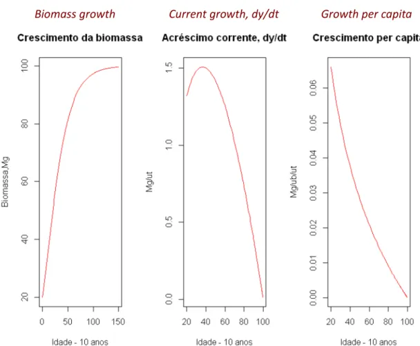
Biomass growth Current growth, dy/dt Growth per capita

Figure 4.3. An example of the application of the EGZ. Simulation of the total biomass of an hypothetical small forest of common oak (Quercus robur) that at age 20 has 74 megagrams (Mg). ub= units of biomass; ut= units of time. The age of the maximum current increment is 22 years. Obtained with software R

4.4.2 The Ageing Perspective

Let assume that the resources do not constrain the growth of an organism, and it is proportional to the size of the population. This assumption leads to the differential equation of the exponential growth:

As a complementary hypothesis we assume that with age the organisms becomes less ef-ficient. This ageing effect causes the exponential declining of r:

(4.13) with the initial condition r=r0 , at aget=0

r=r0 exp(-ct) (4.14)

(45)

(4.15)

To solve this equation we write::

(4.16)

integrating gives

(4.17)

Thus

y=y(0) exp(r(0)(1-exp(-c t))/c) (4.18)

Coherently, the limit of equation (4.18( when c→0 is an exponential:

y= y0 exp(r0t) (4.19)

Given equation (4.16), when t→∞ we get:

yf=y0 exp(r0/c) (4.20)

Replacing equation (4.19) in equation (4.18) we obtain a alternative form of the EGZ:

y=yfexp(-r0/c exp(-ct)) (4.21)

As exp(-r0/c)=1/exp(.r0/c)=y0/(y0 exp(.r0/c))=y0/yf=R, we write:

y= yf Rexp(-ct) (4.22)

Given the two different deductions of the EGZ, we may admit that both organisms, and populations have Gompertzian dynamics.

For small values of t (initial growth) as exp(-ct)≈1-ct, thus 1-exp(-ct)=ct. This implies expo-nential growth, and thus:

y=y0 exp(-r0/c) (4.23)

Theoretical ecology. A unified approach

Theoretical Ecology

A Unified Approach

Second Edition

Luís Soares Barreto

Theoretical Ecology

Theoretical Ecologyy

Theoretical Ecology

A Unified Approach

Theoretical Ecology

A Unified Approach

Second Edition

Luís Soares Barreto

© Luís Soares Barreto, 2005, 2017

E-book published by the author

With compliments

In memoriam of my parents,

also

to Sandra Isabel, Luísa Maria,

ecology students, and ecologists

I am grateful to those who contribute

to the existence of ClickCharts, LibreOffice, Maxima,

R, Scilab e wxMaxima

The author

Luís Soares Barreto was borne in 1935, in Chinde, a small

village in the delta of the Zambezi River, in Mozambique.

In this African country, from 1962 till 1974, he did research

in forestry, and he was also member of the faculty of the

Universidade de Lourenço Marques (actual Universidade

Eduardo Mondlane, Maputo), where he started the

teach-ing of Forestry. While member of this university, from

1967 to 1970, he was a graduate student at Duke

Univer-sity, Durham, NC, U.S.A.. From this univerUniver-sity, he

re-ceived his Master of Forestry in Forest Ecology

(1968), and his Ph. D. in Operations Research applied to

Forestry (1970). Since 1975 till March, 2005, he taught at

the Instituto Superior de Agronomia, Universidade de

Lis-boa. From 1975 to 1982, simultaneously, he taught in the

Department of Environmental Sciences of the Universidade

Nova de Lisboa. Here, in 1977, he conceived, and created

a new five years degree in environmental engineering. He

is the only Portuguese who established a scientific theory.

Besides the ecological theory presented in this book, he

proposed also a unified theory for forest stands of any kind

and ecologically sound management practices grounded

on it. The later theory is a particular case of the former

one. His first contact with mathematical or theoretical

eco-logy occurred in the spring of 1968, when he was

gradu-ate student at Duke University, and he attended a course

(mathematical ecology, MBA 591) in North Carolina State

University, at Raleigh, taught by Professor Evelyn C.

Pielou, holding a visitor professorship in this university.

The author taught population dynamics for about twenty

years. Actually, he is jubilee professor of the University of

Lisbon.

Quotations

Contents

1. Introduction

PART I

ISOLATED POPULATIONS

In the first part of the book, I will approach:

Organism and population variables

The dynamic properties of these variables: self-similarity (allometry)

The pattern of growth of organisms and isolated populations: the Gompertz

model

The laws that isolated populations abide

Modelling structured populations

Demography

2 Population Descriptors, and other Basic Concepts

y

3 Allometry

√

4 The Gompertz Equation

y= yf R

(4.11)

y= y0 R

_(4.11)