Estimating a Portugal NAIRU
Eduardo Gutiérrez
January 8, 2016
Nova School of Business & Economics
University of Maastricht
GPEARI, Portuguese Ministry of Finance
Master Thesis developed under the advisory of Professors Francesco Franco and Lenard Lieb.
TABLE OF CONTENTS
1. Introduction ... 3
2. Literature Review ... 3
2.1 NAIRU ... 3
2.2 Alternative measures of unemployment ... 6
3. The use of the NAIRU in a policy context ... 9
4. Approaches for estimating the NAIRU ... 11
5. Empirical results ... 16
6. The Missing Deflation puzzle ... 18
6.1 Anchored expectations ... 19
6.2. Labour Market Slack ... 22
7. Conclusion ... 26
Annex 1. State-space model ... 27
Annex2. Sensitivity of the results ... 30
References ... 31
1.
Introduction
Interest in the Unemployment-inflation relationship has greatly risen during the last two
decades. Gordon (2013) and Watson (2014) have found that cyclical unemployment is a
leading indicator of inflation in the US. However, in the European Union, mainly
policymakers have estimated structural unemployment and analysis of the concept itself
has been scarce.
In this study, I have both estimated the NAIRU in the Portuguese economy and
addressed the “flattening Phillips Curve”. In particular, I have included inflation
targeting and taken into account the change in the labour market structure in Portugal. I
find that the anchored inflation specification improves the traditionally used backward
looking specification and that measures of unemployment including part-time and
marginally attached workers outperform the official u3 unemployment rate.
2.
Literature Review
2.1NAIRU
The non-accelerating inflation rate of unemployment (NAIRU) is the rate of
unemployment at which inflation stabilizes in the absence of any wage-price surprises.
Friedman first argued in 1968 that inflation accelerates (decelerates) when actual
unemployment falls below (rises above) a Natural Rate of Unemployment, but only on a
temporary basis because the relationship is based not on inflation itself, but on an
“unanticipated” inflation (Friedman, 1968). Once unemployment returns to the NRU,
inflation will stabilize at a permanent higher (lower) level.
Since the NAIRU is unobservable, it needs to be estimated for policy analysis.
reduced-form methods (Gianella et al., 2008).
! Structural methods: model the NAIRU as a function of labour and product market
variables and involve estimating a system of equations explaining the wage
setting and price setting behaviour (see, for example, Morrow & Roegers, 2000).
This methodology identifies the specific determinants of structural
unemployment. However, disagreements about the appropriate structural model,
specification issues and statistical identification issues make the estimates too
uncertain.
! Purely statistical methods: split unemployment into a trend component, identified
as the NAIRU, and a cyclical component. The identification of the two
components can be based either on filtering techniques, the most widely used
being the HP filter (Hodrick Prescott, 1997) and the band pass filter (Baxter &
King, 1995), or on statistical methods assuming that trend unemployment
follows a random-walk (Watson, 1986). It is uncorrelated with inflation because
unemployment is the only series used, around which the NAIRU moves, and the
decomposition is based on arbitrary assumptions.
! Reduced-form approach: obtains the NAIRU by identifying the rate of
unemployment consistent with stable inflation in a Phillips Curve equation. In
addition, statistical constraints are imposed in the path of the NAIRU. It is the
most accepted method due to the given unemployment-inflation relationship and
the feasibility of the estimates across countries and periods.
The temporary trade off described by Friedman was captured by the “triangle
model”, which measured the NAIRU in the reduced-form approach by identifying three
pressures and supply shocks (Gordon, 1997).
𝜋−𝜋! =𝐴 𝐿 𝜋!
!!−𝜋!!!
!
+𝛾 𝐿 𝑈!−𝑈!∗ +𝛿 𝐿 𝑧!+𝑒!, (1)
𝑈!∗ =𝑈!
!!
∗ +𝑣!, (2)
where 𝜋 is actual inflation, 𝜋! is expected inflation, 𝑈! is the actual rate of
unemployment, 𝑈!∗ represents the NAIRU, 𝑧! is a vector of supply shock variables, and
𝑒! and 𝑣! are serially uncorrelated error terms.
The model is a common benchmark to compute the NAIRU. However, the
characteristics of the different factors may vary depending on the theoretical
specification as reflected by different studies:
Expectations have traditionally been based on a backward-looking Phillips curve,
where inertia is formed using recent inflation outcomes (see, for example, Fabiani &
Mestre, 2004; Centeno et al., 2010). The assumption of adaptive expectations derives
from the fact that inflation has followed a random walk during the last decades.
However, the OECD has updated its model to incorporate the notion that expectations
are anchored around the central bank inflation objective, which reduces the effect of
changes in the unemployment gap on inflation (Clifton et al., 2001). In fact, the
unemployment gap of most of the OECD countries incorporating anchored expectations
has higher statistical significance (Rusticelli et al., 2015).
The NAIRU, determining demand pressures, follows a random walk. This implies
a recognition of the hysteresis effect, which lies on the deterioration of human capital
after prolonged periods of unemployment; reducing their influence on wage bargaining
and, as a consequence, on unemployment (Blanchard & Summers, 1986 and Rusticelli
The measured NAIRU is key for policymakers, as acknowledged in the existing
literature. Economists analyze inflationary developments, the sustainability of fiscal
policy and the need for structural policy using the NAIRU as a benchmark of
sustainable trends in output and employment.
2.2Alternative measures of unemployment
Existing literature quantifying the Natural Rate of Unemployment has used the
official measure of the unemployment rate, U-3. According to the OECD, “to be
considered unemployed an individual must be during the reference period without a
job, taking measures to get work during a specific time period (job search) and
available to start work usually immediately”.
This measure has generally been used because it is an indicator of labour market
slack that involves no value judgement by simply requiring an individual to be
searching for a work and allows employment to measure production including all labour
inputs. Apart from U-3 unemployment, labour market slack is composed of time-related
unemployment and discouragement (OECD, Employment Outlook):
! Labour market slack: measures the insufficiency of the volume of work.
! Time-related unemployment: amount of workers willing and available to work
more hours, as long as they are working less than a specified number of hours.
They are structured in three groups: first, individuals who usually work full time
but are working part-time because of economic slack; second, individuals who
work part time but are working fewer hours because of economic slack; and
those who are working part time because full time could not be found. While the
two first groups are expected to be correlated with the economic cycle, the third
problem.
! Discouraged workers: subset of persons marginally attached to the labour force.
The marginally attached are those persons who are available and willing to
work, and who have looked for a job in the last 6 months, but have not been
actively seeking for the last 4 weeks. As output expands, some of them will join
the labour force; and as unemployment increases some of them will leave the
labour force. This means that, during a recession, the labour resources not being
utilized in the economy might be understated. Among the marginally attached,
the discouraged workers have given a job-market related reason for not looking
for a job.
Although U-3 unemployment has traditionally been a good proxy of labour
market slack in Portugal, the onset of the crisis has varied the structure of the labour
market. More specifically, “while conventional unemployment has almost doubled since
2008, the number of involuntary short-term workers has almost tripled and the number
Figure 1 - Labour Market Slack
Then, as confirmed by the graph above, U-3 unemployment is no longer a good
proxy for labour market slack, and other measures of unemployment should be
analyzed. The alternative unemployment rates produced by the BLS are the following:
U-1 Persons unemployed 15 weeks or longer, as a percent of the civilian labour force
U-2 Job losers and persons who completed temporary jobs, as a percent of the civilian labour force
U-3 Total unemployed, as a percent of the civilian labour force (official unemployment rate)
U-4 Total unemployed plus discouraged workers, as a percent of the civilian labour force plus discouraged workers
U-5 Total unemployed, plus discouraged workers, plus all other persons marginally attached to the labour force, as a percent of the civilian labour force plus all persons marginally attached to the labour force
U-6 Total unemployed, plus all persons marginally attached to the labour force, plus total employed part time for economic reasons, as a percent of the civilian labour force plus all persons marginally attached to the labour force
5
10
15
20
25
2002q1 2005q3 2009q1 2012q3 2016q1
date
Unemployment rate Labour Market Slack
Given the enormous increase of discouraged and part-time workers in Portugal,
the author considers it necessary to quantify the NAIRU using the U-6 and U-5 rates
and compare them to the official unemployment rate.
3.
The use of the NAIRU in a policy context
“Economists analyze future inflation trends, the sustainability of fiscal positions
and the need to undertake structural reforms to permanently reduce unemployment
and for this purpose they need a benchmark to identify and distinguish sustainable
and unsustainable trends in output and unemployment. The NAIRU concept provides
such a benchmark.” (Richardson et al., 2000)
-‐ Monetary policy and inflation:
Structural unemployment is useful for monetary policy if it helps to forecast
inflation developments in the short run. After the 2008 economic crisis, many
economists have tried to solve the so-called “missing deflation puzzle”. They argued
that, given the increase in unemployment in those years, inflation should have decreased
much more than it did to be consistent with the Phillips Curve framework. In fact, the
IMF (2013) stated that the relationship between cyclical unemployment and inflation
had become muted. To explain the missing deflation, Ball and Mazumder (2015)
reasoned that inflation expectations have become more anchored and that inflation
development depends on short-term unemployment, which increased less than total
unemployment.
In addition, Gordon (2013) argued that, although the Phillips Curve has not been
able to capture inflation developments, the triangle model has. Specifically, he forecasts
that supply shocks have a big influence on inflationary developments but are not
included in the Phillips Curve. This means that, as explained in the literature review,
one should consider expectations, supply shocks and demand shocks when analyzing
inflation developments.
-‐ Fiscal policy and medium term assessment:
The general government balance, measured by the difference between revenues
and expenditures, varies with the business cycle. On the revenues side, almost all tax
categories are affected by cyclical fluctuations while the expenditures side tends to
compensate domestic demand changes. This implies that during an economic slowdown
expenditures are higher and taxes lower.
Hence, a measure of the government balance in a cyclically normal situation is
needed. This structural budget balance is calculated using the NAIRU estimation as a
measure of structural labour utilization. The NAIRU determines the output gap as
expressed by Okun´s law. This output gap together with revenue and expenditure
elasticities quantifies the structural budget balance.
-‐ Study determinants of the NAIRU and the scope for future
reforms:
By regressing the obtained NAIRU on its potential determinants, one can obtain
the contribution of these to the NAIRU estimates and learn how to decrease this rate.
Some of these factors are the tax wedge, the real interest rate, the average
unemployment benefit replacement rate and union density. Hence, measuring the
determinants of the reduced form measured NAIRU is a key step for policy
by Gianella et al (2009), who found that, for a sample of 19 OECD countries including
Portugal, the most significant variables in determining the NAIRU are the tax wedge,
the PMR (product market regulation) indicator, and the real interest rate.
4.
Approaches for estimating the NAIRU
As recognized by Staiger, Stock and Watson (1996), the estimation of the NAIRU
is imprecise because the NAIRU is not observable and varies over time. This
uncertainty is explained by three reasons: firstly, the estimation of the parameters is
uncertain; secondly, the NAIRU is stochastic and its determinants are not known with
precision; and lastly, there are a number of potential models to estimate it. In this paper,
three different measurement versions are going to be tested: two of them based on the
reduced form approach and the other based on the statistical approach.
- Reduced-form:
The measurement of the NAIRU proposed in this study is based on the
unobserved components model (see annex 1), which obtains its time-path from the
information contained in a reduced-form Phillips curve. Additionally, the behaviour of
the unobserved variable is defined (see equations 1 and 2).
Following Gordon, the Phillips curve, represented by the “triangle model”,
specifies that inflation changes depend on three factors: supply shocks, demand shocks
and inertia. As recognized by the OECD, the dependent variable could be either price
inflation or wage inflation. Also, Rusticelli and Guichard (2011) propose an alternative
specification for Southern European Countries in which “price inflation barely responds
to unemployment”. They argue that although excessive labour demand might have had
proposition and services inflation have been tested and no improvement in the fit has
been found.
Supply shocks are represented by the change in the inflation rate of food and
energy contemporaneously and the rate of inflation of food and energy with respect to
headline inflation in the previous period. Other possible proxies are the change in real
oil prices and the change in real import prices, but have not been considered due to their
lower explanatory power as regressors of inflation developments. Additionally, the
demand shocks are measured by the difference between the actual rate of
unemployment and the natural rate, where the natural rate of unemployment is allowed
to change over time. Macroeconomic theory emphasizes that in case unemployment is
higher than the natural rate, workers searching for a job will push wages down, thereby
decreasing unemployment. Lastly, inertia measures the effect of previous inflation on
current inflation. Given that, in the long run, inflation is assumed to depend only on
nominal factors, the coefficients of lagged inflation have to be constrained to sum to 1.
This implies that in the absence of supply and demand shocks inflation will remain
constant. However, in this model only 3 lags are included, specification obtained
dropping insignificant lags after applying the information criteria.
In this study, I have tested the specification proposed by Gordon using the number
of lags determined by the selection criteria for the supply and demand shocks and 24
lags for inflation which sum equals to 1 but then lagged inflation suppresses the
explanatory power of the shocks1. I have also tested the model using the lags proposed
by the information criteria for inertia, supply and demand shocks, being the NAIRU
measured robust (see annex 2). Due to this, I have followed the policymakers’
1 “When serial correlation is high and the exogenous variables are heavily trended, the lagged variable will
specification by simplifying the model in terms of the number of variables included,
obtaining a structural approach.
Regarding the equation defining the law of motion of the unobservable variable,
the NAIRU is assumed to follow a random walk. A second law of motion is imposed in
Model 2 capturing the behaviour of the gap between the unemployment rate and the
NAIRU. In both models the path of the NAIRU is derived from the information
contained in the Phillips Curve by means of the Kalman Filter (see annex 1). Then, we
are going to consider two models:
Model 1
To measure the NAIRU we depart from the basic formulation, which includes the
Phillips Curve and the NAIRU equation.
Δ𝜋! = 𝐴 𝐿 ∆𝜋!
!!+𝛽 𝑈!−𝑈!∗ +𝛾𝑧!+𝑒!, (3)
𝑈!∗ = 𝑈! !!
∗ +𝑣!, (4)
where Δ is the first difference operator, 𝜋 is the headline inflation, 𝑈! is the actual
rate of unemployment, 𝑈!∗ represents the NAIRU, 𝑧! is a vector of supply shock
variables, 𝜖! is a serially uncorrelated error term with zero mean and variance 𝜎!!, and
𝑣! is a serially uncorrelated error term with zero mean and variance 𝜎!!.
The Kalman Filter allows for the estimation of the behaviour of the latent
variables and the coefficients simultaneously by maximum likelihood. However, as
recognized by Gordon (2013) and Watson (2014), the variance of the trend equation
error term has to be set artificially. This value is very important because it determines
the signal-to-noise ratio (𝜎!!/𝜎!!), the smoothness of the series. Logically, the higher the
Gordon (1997) suggested choosing a signal-to-noise ratio that allows the NAIRU to
move freely but rules out sharp quarter-to-quarter zigzags. Specifically, he proposed 𝜎!!
= 0.09. However, other authors have proposed different values: for instance, Müller
(2007) estimated that 𝜎!!= 0.28. In this study, I impose 𝜎!! = 0.10, consistent with
Gordon propositions. Higher variance implies an inappropriately high volatility of the
NAIRU. Then, the smoothness of the NAIRU achieved by this specification is an
assumption, making it convenient to compare the result with other models.
Model 2:
This approach relies on the equations defined in the previous specification, the
Phillips curve and the law of motion describing the NAIRU, and adds a second
transition equation specifying the time-path of the unemployment gap. This additional
equation guarantees that the NAIRU does not deviate permanently from the actual
unemployment rate, consistent with a sticky labour market.
𝑈!−𝑈!
∗ =𝜓 𝐿 𝑈!
!!−𝑈!∗!! + 𝜁!, (5)
where 𝑈!−𝑈!
∗is the unemployment gap and 𝜁! is a serially uncorrelated error
term with zero mean and variance 𝜎
!!. Following Jaeger and Parkinson (1994), two lags
of the unemployment gap are included. The sum of the autoregressive parameters varies
between 0.75 and 0.9 (Rusticelli & Guichard, 2011), having imposed in this study that
the sum equals to 0.85.
With respect to the smoothness of the series, it is now determined by both the
relative variance of the error of the NAIRU transition equation with respect to the
variance of the error of the Phillips Curve equation and the relative variance of the error
equation. The higher the latter the more volatile the NAIRU series will be. The Kalman
filter methodology has been used to quantify the parameters and the unobserved
variables by maximum likelihood.
-Statistical
HP filter:
Numerous papers have tried to explain inflationary developments using the
Hodrick-Prescott (HP) filter to statistically measure the trend of the unemployment rate
and have used the difference between the actual unemployment rate and the HP filtered
trend unemployment rate as the demand shock in equation 3. In this paper, the HP filter
NAIRU estimates are derived using a 𝜆 of 6400. Although typically the parameter is
assumed to be 1600 when using quarterly data, I assume 6400 following Gordon
because it yields a smoother trend.
Seeing as the unemployment series is composed of a trend component 𝑡𝑟! and a
cyclical component 𝑐!, Hodrick and Prescott (1997) argue that we can obtain the trend
component by solving the following problem:
𝑀𝑖𝑛 !"
! (𝑢!−𝑡𝑟!)
!
!
!!!
+𝜆 ( !!!
!!!
∇!𝑡𝑟!!
!)! ,
(6)
where ∇ is the difference operator and 𝜆 determines the smoothness of the trend
5.
Empirical results
The results obtained in all the models are consistent with economic theory: the
unemployment gap is negatively related to inflation. The goodness of fit of the models
has been evaluated using the Akaike Information Criteria2. We see in table 2 that in
model 2 the NAIRU performs better than in the other two specifications, which means
that it explains the data better.
2 The AIC determines the best model in terms of the likelihood function adjusted by the number of
parameters. The best model is the one with the lowest AIC.
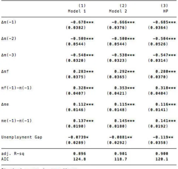
Table 2- Estimated Phillips Curve using the alternative models unemployment gaps
The HP-filter specification measures an unemployment gap that is statistically
significant at the 95% level. However, it is based on arbitrary assumptions commoving
excessively with the actual unemployment rate (see Figure 2). We see in Figure 3 that
demand pressures in the aftermath of the recession were lower according to the HP
filter. It seems more plausible that the macroeconomic adjustment implied higher
demand pressures consistent with the Kalman Filter specifications.
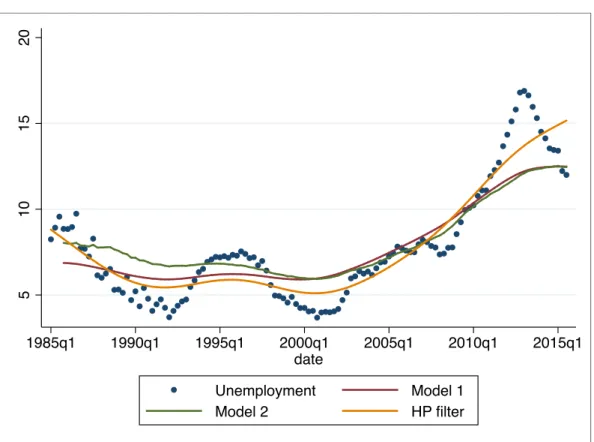
Figure 2 - NAIRU estimates from the three models
Figure 2 depicts the observed unemployment rate and the estimated NAIRU. The
NAIRU varies considerably less than the Unemployment rate and displays an upward
tendency beginning in 2000. Specifically, model 2 indicates that it increased from 6%
in 2000 to 8.45% in 2007 to 12.3% in 2013. The increase of the NAIRU in the period
2007-2013 is remarkable. Carneiro, Portugal and Varejao (2013) identify three main
channels that might have amplified the employment response to the great recession in
5
10
15
20
1985q1 1990q1 1995q1 2000q1 2005q1 2010q1 2015q1
date
Unemployment Model 1
Portugal: credit constraints faced by Portuguese firms, rigidity of wages to respond to
negative demand shocks and segmentation of the labour market being those employed
with temporary contracts the most affected by the recession.
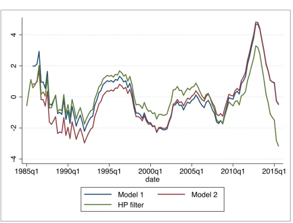
We see in Figure 3 that also demand pressures increased a lot during the period
2007-2013, which means that the Unemployment rate increased more than the
NAIRU. However, since then the Unemployment rate started to decrease while the
NAIRU has remained around 12%.
Figure 3- Unemployment Gap estimates from the three models
6.
The Missing Deflation puzzle
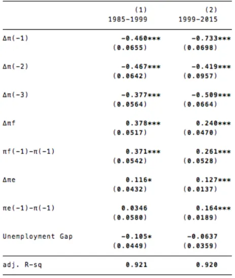
Comparing results in 1985-1999 and 1999-2015, we see that the effect of the
shocks is generally lower in the second period, and specifically, that the unemployment
gap coefficient decreases from -0.105, significant at the 90% level, to -0.0637, not
significant (see table 3). As explained before, it has been argued that the Phillips Curve
-4
-2
0
2
4
1985q1 1990q1 1995q1 2000q1 2005q1 2010q1 2015q1 date
has flattened and this result would confirm this theory. Then, I have included the recent
developments in Portugal and compared the results. First, I have incorporated anchored
expectations to the model in the context of the European Monetary Union´s 2% inflation
target; and then I have considered alternative measures of labour slack consistent with
increasing discouraged and part-time workers in the Portuguese economy.
6.1 Anchored expectations
One possible explanation for the change in the explanatory power of demand and
supply shocks on inflation developments is inflation targeting. Since the creation of the
Table 3- Comparison of different periods estimation of the Phillips Curve
European Monetary Union in 1999, policymakers have given high emphasis to keeping
inflation at the 2% level. This should be considered by including the difference between
the Euro-area inflation rate and an inflation target in the Phillips Curve:
Δ𝜋!= 𝐴 𝐿 ∆𝜋!
!!+𝛽 𝑈!−𝑈!∗ +𝛾𝑧!+𝜃𝐷𝑈(𝜋!",!!!−𝑇𝐴𝑅)+𝑒!, (7)
where DU is a dummy taking the value of 0 before inflation targeting started and
1 after it is anchored around the central bank target (1999), TAR is the central bank
inflation target and 𝜋!" is the euro area inflation rate.
The difference between the euro area inflation rate and the target set by the ECB
is statistically significant. In addition, when I take into account inflation targeting the
coefficient of the demand shock increases from -0.0637 to -0.0687 in the period
1999-2015 and is significant at the 90% confidence level. This partly explains why inflation
did not fall more during the crisis after the high increase in unemployment: inflation
targeting offset the effect of the increase in unemployment. In fact, “better anchored
expectations has been recognized as the main reason for more stable inflation and the
absence of disinflation in the aftermath of the financial crisis” (Rusticelli et al., 2015).
The NAIRU estimated using this alternative specification has been lower than the
one estimated using backward-looking inflation expectations since the beginning of the
crisis (see Figure 4). This provides evidence that demand pressures might have been
underestimated due to inflation targeting.
Figure 4 – NAIRU estimates with Anchored expectations
5
10
15
20
1998q1 2002q3 2007q1 2011q3 2016q1
date
6.2. Labour Market Slack
As I have remarked in the first section, labour market slack refers to the
insufficiency of work and not only covers those who are not working and searching for
a job but also those who are working part-time for economic reasons and those who are
not searching for a job but would like to work. These have to be tested because they are
important for policy recommendations and might provide a more precise inflation
forecast.
Part-time workers are expected to exert a higher pressure on wages than the
unemployed, and Centeno, Maria and Novo (2010) have shown that, in Portugal, the
probability of a marginally attached worker obtaining a job is almost the same as that of
an unemployed worker, and attribute the difference in the probability of transitioning to
inactivity (see Figure 5). For this reason, discouraged workers should also be included
when using the NAIRU to define future reforms.
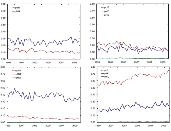
Figure 5-Transition rates. Source: Centeno et al., (2010)
The graphs show the probability of employed (E), unemployed (U), marginally
attached (M), and non-activity workers (N) getting to each of the other states between
1999 and 2009.
Considering the analysis above, two additional labour slack measures are going to be
used to measure the NAIRU: the U-5, that includes U-3 unemployed plus marginally
attached workers, and the U-6, that considers U-3 unemployed, marginally attached and
Figure 6- Alternative Unemployment Measures
The NAIRU measured with the alternative unemployment measures is the
following:
Figure 7- NAIRU estimates, alternative Unemployment measures
5
10
15
20
25
2002q1 2005q3 2009q1 2012q3 2016q1
date
U-3 U-5
U-6
5
10
15
20
st
a
te
s,
t
re
n
d
,
smo
o
th
2002q1 2005q3 2009q1 2012q3 2016q1 date
U3 U6
The effect of the demand shock on inflation developments is higher and more
significant when measured with the U-6 Unemployment rate. Also, the Akaike
Information Criteria indicates that U6 Unemployment captures the data better. This
means that discouraged and part time workers might be considered in the
Unemployment measurement both for a better explanation of the inflation progress and
in order to include these in the scope for future reforms. Also, U-5 Unemployment,
adding only marginally attached workers to the official rate, performs better than the
official rate (see table 5).
7.
Conclusion
The NAIRU is a key concept in macroeconomic policy but unfortunately no consensus
has been reached as to how it should be measured. Anyway, the “triangle model”
proposed by Gordon has been widely accepted because it is very precise. This
methodology has been applied to the Portuguese case and two alternatives to better
capture inflation developments have been proposed: inflation anchoring and more
complete measures of slack in the labour market.
The primary objective of the Eurosystem is to maintain price stability in the euro area
and it is key to include inflation targeting in the estimation of the NAIRU. In fact, we
have seen that inflation targeting is significant at the 99% level and determines a lower
NAIRU which means that demand pressures were higher than initially computed. More
workers with more influence have been affecting prices since the outburst of the crisis
to a greater degree than has been expected by the traditional model because inflation
targeting has kept inflation low.
Also, including part time and marginally attached workers in the labour
insufficiency rate improves the results. The traditional specification was not capturing
the development of the Portuguese labour market, characterized by a huge increase in
discouraged and part time workers. The exclusion of part time workers might be
acceptable due to the difficulty of measuring them but given the similar probability of
transitioning to employment of marginally attached and unemployed workers, they
Annex 1. State-‐space model
For Kalman filter estimation, the model is expressed in its state-space form,
composed by a measurement and a state equation:
𝑌!= 𝐷𝑧!+𝐹𝑤!+𝐺𝑣!,
𝑧!= 𝐴𝑧!!!+𝐶𝜖!,
where 𝑌! is an observed endogenous variable, 𝑤!is a vector of observed
exogenous variables, D, F, A, C and G are matrices of time-invariant parameters, 𝑧! is a
vector of unobserved parameters and 𝑣! and 𝜖! are white noise error terms.
The measurement equation derives from theoretical grounds; in this case, the
Philips curve determines the relationship between unemployment and inflation. On the
other hand, the transition equation contains atheoretical laws of motion describing the
behaviour of the unobservable variable.
The Kalman filter is a recursive procedure for computing the optimal estimator
(thus, minimizing the mean square error) at time t based on the information available at
that time. Starting with an assumed initial unobservable variable 𝑧!, 𝑌! is predicted;
then using the observed value of 𝑌! the prediction error is computed. Lastly, this
prediction and the state equation errors are used to obtain the unobserved variable.
The algorithm adopted for the system estimation was the SSPACE procedure
available in the econometrics package STATA. The following state space systems have
Model 1
Measurement equation:
∆𝜋!=𝐴 𝐿 ∆𝜋!
!!+𝛽 𝑈−𝑈∗ +𝑦𝑧!+𝑒!,
𝑈=𝑈∗+ 𝑈−𝑈∗ ,
which can be expressed in the matrix explained above as:
∆𝜋! 𝑈 =
0 −𝛽
1 1
𝑈∗
𝑈!−𝑈!∗ + 𝑎
! 𝑎! 𝑎! 𝑏! 𝑑! 𝑒! 𝑓!
0 0 0 0 0 0 0
∆𝜋! !!
∆𝜋! !! ∆𝜋!
!!
∆𝜋! (𝜋!
!!
! −𝜋!
!!) 𝛥𝜋!
(𝜋! !! !
−𝜋! !!)
+ 1 0 0 0
𝑒!
0 ,
where the variance-covariance matrix of 𝑒!
0 is: Σ!!=
𝜎! ! 0
0 0 .
State equation:
𝑈!∗=𝑈! !!
∗ +𝜈!,
𝑈!−𝑈!∗=𝜁! ,
which can be expressed in the matrix form explained above as:
𝑈∗ 𝑈−𝑈∗ =
1 0 0 0 𝑈! !! ∗ 𝑈!
!!−𝑈!∗!!
+ 1 0
0 1
𝜈!
𝜁! ,
Where the variance-covariance matrix of 𝜈!
𝜁! is: 𝛴!!=
𝜎! ! 0
Model 2:
Measurement equation:
∆𝜋!=𝐴 𝐿 ∆𝜋!
!!+𝛽 𝑈−𝑈∗ +𝑦𝑧!+𝑒!,
𝑈=𝑈∗+ 𝑈−𝑈∗ ,
which can be expressed in the matrix explained above as:
∆𝜋! 𝑈 =
0 −𝛽 0
1 1 0
𝑈∗ 𝑈!−𝑈!∗
𝑈!
!!−𝑈!∗!!
+ 𝑎! 𝑎! 𝑎! 𝑏! 𝑑! 𝑒! 𝑓! 0 0 0 0 0 0 0
∆𝜋!
!! ∆𝜋!
!! ∆𝜋!
!! ∆𝜋! (𝜋!
!!
!
−𝜋!!!) Δ𝜋! (𝜋!
!!
!
−𝜋! !!)
+ 1 0
0 0
𝑒!
0 ,
Where the variance-covariance matrix of 𝑒!
0 is: Σ!!=
𝜎! ! 0
0 0 .
State equations:
𝑈!∗=𝑈!
!! ∗ +𝜈!,
𝑈!−𝑈!∗=𝜓(𝐿)(𝑈!
!!−𝑈!∗!!) +𝜁! ,
which can be expressed in the matrix form explained above as:
𝑈∗
𝑈!−𝑈!∗
𝑈!
!!−𝑈!∗!! =
1 0 0 0 𝛿
! 𝛿!
0 1 0
𝑈!
!! ∗ 𝑈!
!!−𝑈!∗!!
𝑈!
!!−𝑈!∗!! +
1 0 0
0 1 0
0 0 0
𝜈!
𝜁! 0
,
Where the variance-covariance matrix of
𝜈! 𝜁! 0
is: Σ!!=
𝜎! ! 0 0
0 𝜎! ! 0
0 0 0 .
Annex2. Sensitivity of the results
Studies measuring the NAIRU differ in the number of lags selected for demand
and supply shocks. There are three approaches: selection based on theoretical grounds,
on the information criteria and select the number of lags proposed by the information
criteria and drop the insignificant ones. Studies trying to validate the NAIRU concept
use the second approach and use typically 4 lags of the inertia, supply and demand
shocks (complete approach). However, most of the NAIRU estimation studies impose
the demand shock on theoretical grounds selecting only 1 lag and the supply shocks
using either the first or the last option.
I have selected in this study the first approach because of its feasibility for policy
analysis and the robustness of the model under the different specifications. In fact, in
the next graph I compare the NAIRU that I have estimated in the paper (structural) with
the complete approach estimation and they are almost identical.
Figure A1- Sensitivity of the NAIRU
5
10
15
20
1985q1 1990q1 1995q1 2000q1 2005q1 2010q1 2015q1 date
References
Achen, C.H. (2000). Why Lagged Dependent Variables Can Suppress the Explanatory
Power of Other Variables." Ann Arbor 1001:48106-1248.
Ball, L. and Mankiw, N. (2002). The NAIRU in Theory and Practice. Journal of
Economic Perspectives, 16(4), pp.115-136.
Ball, L. and Mazumder, S. (2015). A Phillips Curve with Anchored Expectations and
Short-Term Unemployment. IMF Working Papers, 15(39), p.1.
Baxter, M. and King, R. (1999). Measuring Business Cycles: Approximate Band-Pass
Filters for Economic Time Series. Review of Economics and Statistics, 81(4),
pp.575-593.
Blanchard, O. and Summers, L. (1986). Hysteresis and the European Unemployment
Problem. NBER Macroeconomics Annual, 1, p.15.
Boone, L., Turner, D., Rae, D., Giorno, C., Meacci, M. and Richardson, P. (2002).
Estimating the structural rate of unemployment for the OECD countries. OECD
Economic Studies, 2001(2), pp.171-216.
Carneiro, A., P. Portugal and J. Varejao (2013), Catastrophic Job Destruction, IZA
Discussion Papers No 7670, Institute for the Study of Labor (IZA)
Centeno, M., Maria, J. and Novo, Á. (2010). How to measure unemployment?
Implications for the NAIRU. Banco de Portugal.
Clifton, E., Hyginus, L. and Wong, C. (2001). Inflation Targeting and the
Unemployment- Inflation Trade-off. IMF Working Paper 01/166.
NAIRU. Empirical Economics, 29(2), pp.311-341.
Friedman, A. and Suchoy, T. (2004). The NAIRU in Israel: an unobserved components
approach. Israel Economic Review, 2(2), pp.125-154.
Friedman, M. (1968). The Role of Monetary Policy. American Economic Review.
Gianella, C., Rusticelli, I., Koske, E. and Chatal, O. (2008). What Drives the NAIRU:
Evidence from a Panel of OECD Countries Paris. OECD Department Working
Paper, No. 649.
Gordon, R. (1997). The Time-Varying NAIRU and its Implications for Economic
Policy. Journal of Economic Perspectives, 11(1), pp.11-32.
Gordon, R. (2013). The Phillips Curve is Alive and Well: Inflation and the NAIRU
During the Slow Recovery. NBER.
Hodrick, R. and Prescott, E. (1997). Postwar U.S. Business Cycles: An Empirical
Investigation. Journal of Money, Credit and Banking, 29(1), p.1.
IMF, (2013). The Dog that didn't Bark: Has Inflation been muzzled or was it Just
Sleeping.
IMF, (2015). IMF Country Report: Portugal. Washington, D.C.
Morrow, K. and Roegers, W. (2000). Time Varying NAIRU/NAWRU estimates for the
Euro-area member states. European Communities.
OECD, (2014). OECD Employment Outlook.
Phelps, E. (1967). Phillips Curve Expectations of Inflation and Optimal Unemployment
Pichelmann, K. and Schuh, (1997). The NAIRU-Concept: A Few Remarks. OECD
Economics Department, No. 178.
Rusticelli, E. and Guichard, S. (2011). Reassessing the NAIRUs after the crisis. OECD
Economics department, 918.
Rusticelli, E., Cavalleri, M. and Turner, D. (2015). Incorporating anchored inflation
expectations in the Phillips curve and in the derivation of OECD measures of the
unemployment gap. OECD Journal: Economic Studies, 2015(1), pp.299-331.
Staiger, D., Stock, J. and Watson, M. (1997). The NAIRU, Unemployment and
Monetary Policy. Journal of Economic Perspectives, 11(1), pp.33-49.
Watson, M. (1986). Univariate detrending methods with stochastic trends. Journal of
Monetary Economics, 18(1), pp.49-75.
Watson, M. (2014). Inflation Persistence, the NAIRU, and the Great Recession.