!
"#$%& $'( ) ) *
!
"#$%& $'( ) ) *
!
!
"
!
# $
!
This paper concerns the numerical simulation of internal recirculating flows encompassing a two dimensional viscous incompressible flow generated inside a regularized square driven cavity and over a backward facing step. For this purpose, the simulation is performed by using the projection method combined with a Chebyshev collocation spectral method. The incompressible Navier Stokes equations are formulated in terms of the primitive variables, velocity and pressure. The time integration of the spectrally discretized, incompressible Navier Stokes equations is performed by a second order mixed explicit/implicit time integration scheme. This scheme is a combination of the Crank Nicolson scheme operating on the diffusive terms and a second order Adams Bashforth scheme acting on the advective terms. The projection method is used to split the solution of the incompressible Navier Stokes equations in two decoupled problems: the Burgers equation to predict an intermediate velocity field and the Poisson equation for the pressure, which is used to correct the intermediate velocity field and satisfy the continuity equation. Numerical simulations for flows inside a two dimensional regularized square driven cavity for Reynolds numbers up to 10000 and over a backward facing step for Reynolds numbers up to 875 are presented and compared with numerical results previously published, where good agreement is demonstrated.
: regularized square driven cavity, backward facing step, chebyshev collocation spectral method, incompressible Navier Stokes equations, projection method
1
Internal recirculating flows generated within a bounded domain are very important under a technological perspective and also of a great scientific interest because they display several aspects of fluid mechanical phenomena in a very simple geometrical setting. Thus, corner vortices, longitudinal vortices, transition, and turbulence all occur naturally and can be studied in the same closed geometry (Shankar and Deshpande, 2000).
Numerical simulations of the Navier$Stokes equations for studying two$dimensional flows of incompressible viscous fluid are generally based upon a primitive variables formulation (velocity and pressure) or vorticity$streamfunction formulation. The major difficulty arising with the former formulation comes from the coupling of the pressure with the velocity, to satisfy the incompressibility condition. The continuity equation contains only velocity components, and there is no direct link with the pressure as it happens for compressible flow through the density (the lack of
evolution equation for the pressure in primitive variables
formulation is the source of difficulty). The use of a vorticity$ streamfunction formulation of the equations avoids this problem. However, although its application to two$dimensional flows is quite common, the extension to three$dimensional problems is not straightforward. Thus, the primitive variables formulation is preferable because it is easily extended to three dimensions.
Several methods were proposed to overcome the difficulty arising in the primitive variables formulation. Among these, the projection methods or fractional steps methods (splitting methods) gained a new interest because of theirs non iterative nature, no requirement of any specific memory storage and appropriate use for simulation of unsteady incompressible flows. These methods belong to the predictor$corrector algorithms, where the pressure acts as a projection of the predicted velocity field (intermediate velocity field) onto a divergence$free space. In fact, there are several variants of the original projection method proposed by Chorin (1968) and Temam (1968). However, the use of projection methods has been
' " ( ) * + ," "
popularized associated to finite difference, volume or finite element methods, and there are few applications reported on spectral methods (Huges and Randriamampianina, 1998).
The main objective of this paper is to develop an efficient
numerical method for the solution of a two dimensional
incompressible viscous fluid with internal recirculating flows generated inside a bounded geometry. For this purpose, the numerical solution of incompressible Navier$Stokes equations in two dimensions (INSE2D) is based upon a Chebyshev collocation spectral method (also named Chebyshev pseudospectral method) in conjunction with a second$order projection method and coupled with appropriate boundary conditions. The motivation for using collocation spectral methods stems from their high precision and very low phase errors for the prediction of time$dependent flow regimes. A time integration of the equations system is performed by using a semi$implicit second$order accurate scheme (second$order Adams$Bashforth and Crank$Nicolson).
Spectral methods have been used in combination with temporal schemes of high order (at least order three). For example, Botella (1997) used a temporal scheme of order three, to improve the accuracy of his algorithm that involved a variant of the projection method with a pseudospectral method. In the present paper the algorithm is based on an original combination that involves the projection method with a semi$implicit temporal discretization of second order (which guarantees a good stability of the method) in a structure of spectral collocation. This numerical algorithm uses the technique of the complete diagonalization (non$iterative technique) which is very effective and fast for the direct solution of the resulting equations after the spatial and temporal discretization.
the resulting equations, after the application of the projection method. In the following section the numerical results related to the two benchmark problems are presented and compared with numerical results previously published. The last section presents the conclusions.
i
c = coefficients to evaluate the first derivate matrix D(1) )
1 (
D = Chebyshev collocation first derivative matrix )
1 ( ik
D = coefficients of matrix D(1)
H = 1, non dimensional channel height 2
H/ = non dimensional channel step height 1
s
H = horizontal extension at the bottom left of the secondary vortices
2 s
H = horizontal extension at the bottom right of the secondary vortices
3 s
H = horizontal extension at the top left of the secondary vortices
) (x
hi = Lagrange polynomials
L=30H, longitudinal non dimensional channel length c
L = characteristic length (either length of the square cavity or channel height,H)
N = number of polynomials or collocation points in x
M = number of polynomials or collocation points in y b
N = number of points indicating the starting of the Buffer zone
x
N = number of points indicating the position of the outflow boundary
P= 2
0
U
P ρ , non dimensional pressure field
P = dimensional pressure field
Re =U0Lc ν, Reynolds number characteristic of the flow
j
s = general filter function
t =tU0 Lc, non dimensional time t = dimensional time
u
= non dimensional horizontal component of velocity0
U = dimensional reference velocity
) (x,t
uN = polynomial approximation of degree N of the function u(x,t)
) (t
uˆk = time dependent expansion spectral coefficients
v = non dimensional vertical component of velocity
V =V U0=(u,v), non dimensional velocity vector
V~ = non dimensional intermediate velocity vector at time
t n 1)
( +
V = dimensional velocity vector 1
s
V = vertical extension at the bottom left of the secondary vortices
2 s
V = vertical extension at the bottom right of the secondary vortices
3 s
V = vertical extension at the top left of the secondary vortices
x =x Lc, non dimensional horizontal coordinate
x = dimensional horizontal coordinate i
x = Chebyshev Gauss Lobatto points c
x = horizontal position of the primary vortices
1 s
x = horizontal position at the bottom left of the secondary vortices
2 s
x = horizontal position at the bottom right of the secondary
vortices
3 s
x = horizontal position at the top left of the secondary vortices
y =y Lc, non dimensional vertical coordinate
y= dimensional vertical coordinate c
y = vertical position of the primary vortices
1 s
y = vertical position at the bottom left of the secondary vortices
2 s
y = vertical position at the bottom right of the secondary vortices
3 s
y = vertical position at the top left of the secondary vortices
w
= boundary velocity0
w = initial velocity field )
(x
Tk =cos(kcos 1x)
− , Chebyshev polynomials of order k
) (x
TN′ = first order derivative of the Chebyshev polynomial of order N, TN(x)
t = non$dimensional time step
c
t = non$dimensional critical time step
ν
= kinematic viscosityω = vorticity
ρ = density
) (x
k
φ = basis functions
ψ = stream function
= internal computational domain
∂ = boundary of domain
℘
= projection operatorik
δ = Kronecker delta operator
τˆ = unitary vector tangent to the boundary
nˆ = unitary vector normal to the boundary
∇ = gradient operator
2
∇ = Laplacian operator
) 2 ( ) 1
( , = order of the first and second derivative
1 1 + − n n n
,
, = variables evaluated at time t, t− t,t+ t
= indicates derivative with respect to x
k
i, = relative to the number of polynomials or collocation
points
Two$dimensional viscous incompressible fluid flows are
governed by the Navier$Stokes equations. The dimensionless unsteady Navier$Stokes equations for incompressible flows in Cartesian coordinates may be written in primitive variables as
V P
V . V t
V 2
Re 1 )
( ∇ =−∇ + ∇
+ ∂ ∂
in (1)
0
=
where the unknowns are the vectorV, which represents the velocity
of the flow and the scalar P, which represents the pressure field.
Here,
Re
is the Reynolds number of the flow,U0 is the referencevelocity, Lc represents the characteristic length and ν the
kinematical viscosity. Let be the internal computational domain
with sufficiently smooth boundaries ∂ . The initial condition is
given as
o w
V t=0= in (3)
satisfying Eq. (2) (the initial velocity field wo is solenoidal).
Equations (1) and (2) are completed with an appropriate boundary condition for the velocity field,
w
V = on ∂ (4)
The Navier$Stokes equations were non$dimensionalized using the following dimensionless variables:
0 2
0
0, ,
, ,
U V V U P P L U t t L
y y L
x x
c c c
= =
= = =
ρ (5)
The major difficulty to solve numerically the incompressible Navier$Stokes equations (INSE) arises from the fact that the
velocity V and the pressure
P
are coupled together by theincompressibility constraint (Eq. (2)). To overcome this difficulty, Chorin (1968) and Temam (1968), proposed the projection method (or fractional step method), which decouples the velocity and the pressure fields. The projection method has been widely used and has proven to be very efficient for this type of problem.
These classes of methods permit to uncouple the velocity and the pressure in each time step by reducing the solution of the Navier$Stokes equations to the solution of two successive problems. The first step solves an intermediate velocity, which does not satisfy the incompressibility condition (the velocity field is not solenoidal), while in the second step the intermediate velocity is projected onto a divergence$free space. This last step is equivalent to the solution of a Poisson equation for pressure, which is used to correct the intermediate velocity in order to fulfill the incompressibility condition.
The projection methods are based on the observation that the left$hand side of Eq. (1) is a Hodge decomposition. Hence an equivalent projection scheme is given by
− ∇ + ∇
℘ = ∂ ∂
V V
. V t
V 2
Re 1 )
( (6)
where℘is the operator which projects a vector field onto the space
of divergence$free vector fields with appropriate boundary
conditions.
The projection
℘
can be defined by the solution of a Poissonequation. Specifically, let W=V+∇φ be the Hodge decomposition
of W, where
φ
is a scalar field and Vis the divergence$freevelocity field that is required to satisfyV∂ =w. Then, in order to
determineV fromW let (Brown, Cortez and Minion, 2001):
φ
∇ − = ℘
= W W
V ( ) (7)
where
W . ∇ =
∇2φ in (8)
) ( ˆ
ˆ. n. W w
n∇φ= − on ∂ (9)
Following Streett and Macaraeg (1989/90), the semi$discretized version of a semi$implicit projection method applied to Eqs. (1) and (2) can be written in two steps as follows:
a. The advection$diffusion step solves the intermediate velocity field at time(n+1) t,V~ by
) ( ) ( Re
1 ~
V NL V D t
V
V − n = −
in (10)
with the intermediate boundary conditions
) 2
( ˆ ˆ ~
ˆ.V=τ.V+τ. t ∇Pn−∇Pn−1
τ on ∂ (11)
.V n V .
nˆ ~= ˆ on ∂ (12)
where NL(V)=(V.∇)V and D(V)=∇2V represent the
advection and diffusion terms.
b. The pressure correction step solves the Poisson equation for 1
+
n
P from
t V . Pn
~ 1
2 =∇
∇ + in (13)
with the homogeneous Neumann boundary condition:
0 ˆ.∇Pn+1=
n on ∂ (14)
Then the velocities are updated with
1
1 ~ +
+ = − ∇ n
n V t P
V in +∂ (15)
This step can be viewed as the projection of the velocity field onto the divergence$free space. At the end of the full step there exists a nonzero tangential component of the velocity on the boundary.
The magnitude of this finite slip velocity can be reduced by a
proper choice of the intermediate boundary condition onV~ (Streett
and Macaraeg, 1989/90). The slip velocity may be reduced to )
( t3
O through the boundary condition for the intermediate
tangential velocity component, Eq. (11). This intermediate boundary condition is obtained from the Eq. (15) with an expansion of the
term ∇Pn+1in Taylor series about t=tn and an approach of finite
differences of the term∇Ptn(see Streett and Macaraeg, 1989/90).
! "
) ( 2 1 ) ( 2 3 )
(V = NLVn − NLVn−1
NL (16) 2 )] ( ) ~ ( [ ) ( n V D V D V
D = + (17)
Equations (16) and (17) are substituted in the Burgers equation (Eq. (10)), and at each time step, the solution of the problem reduces to the resolution of Burgers and Poisson equations.
! "
Equations obtained from the semi$discretized version of the projection method are spatially discretized using a Chebyshev collocation spectral method. The collocation spectral method is characterized by the fact that the numerical solution is forced to satisfy the governing equations exactly at collocation points. So, the series expansion for a function u(x,t) on the domain[−1,1] may be approximated as ) ( ) ( ˆ ) , ( 0 x t u t x
u N k
k k
N
∑
φ=
= (18)
where the φk(x) are the trial functions (also known as basis
functions) and the uˆk(t) are the time dependent expansion spectral
coefficients.
For a Chebyshev collocation method, the functions φk(x) are
the Chebyshev polynomials of orderk,Tk(x);
) ( ) ( ˆ ) , ( 0 x T t u t x u k N k k N
∑
= = (19)and the interpolation points are the so$called Chebyshev$Gauss$ Lobatto points, ,..., N , i N i
xi cos =0 1
= π (20)
which correspond to the extreme points of the Chebyshev
polynomials of order N,
) cos cos( )
(x N 1x
TN = − (21)
The expansion coefficients, uˆk(t) may be evaluated by the
inverse relation ,..., N , k N i k c t x u Nc t u N i i i N k
k cos , 0 1
) , ( 2 ) ( ˆ 0 = =
∑
= π (22)whereciand ck=1fori,k=1,2,..,N−1and c0=cN =2.
The collocation spectral method can be seen as a technique of interpolation, so Eq. (19) also can be expressed in terms of Lagrange polynomials de order N, hi(x) such that hi(x)=δik, which is the Kronecker operator. The Lagrange polynomials for the Chebyshev$ Gauss$Lobatto points (Eq. (20)) may be represented by the expression: N ,..., , i , x x N c x T x x h i i N i
i 01
) ( ) ( ) 1 ( ) 1 ( ) ( 2 2 1 = − ′ − −
= + (23)
where ci =1 for i=1,..,N−1 and c0=cN =2, (Canuto et al.,
2006; Peyret, 2002).
The differentiation step can be accomplished in the transformed
space (“transform method”) or in physical space (“matrix
multiplication method”). The first method is performed efficiently by means of a fast cosine transform with a recurrence relation in spectral space (see Canuto et al., 2006; Martinez, 1999) and the second method is based on explicit expressions obtained by differentiating the Lagrange polynomials. The matrix multiplication method is used in this paper because it is very efficient and easy to implement.
The spatial derivative of uN(x,t) at the collocation points
x
i isevaluated using the analytical derivative of the Lagrange
polynomials,
∑
= = = ′ N k k ) ( ik iN x,t D u x ,t , i ,,...,N u
0
1 ( ) 01
)
( (24)
where D(1) is the Chebyshev collocation derivative matrix. This
matrix D(1) is given by the following expression:
= = + − = = + ≤ = ≤ − − ≠ − − = + N. k i , N , k i , N , N k i , ) x x k, i , ) x x ( c ) c D k k k i k k i i ) ( ik 6 1 2 0 6 1 2 1 1 1 ( 2 1 ( 2 2 2 1 (25)
This expression is easily found in the literature of the spectral methods (Boyd, 2001; Canuto et al., 2006; Deville et al., 2002; Peyret, 2002; Solomonoff and Turkel, 1989; Trefethen, 2000). The
Chebyshev collocation second derivative matrix D(2) can be
obtained analytically using an explicit expression (see Peyret, 2002) or by the following relationD(2)=(D(1))2.
The results presented so far can be readily extended to two$
dimensions. If an unknown matrix U is defined such that
ij j
i,y ) u
x (
U = , then the partial derivatives of the interpolant
evaluated at the collocation points, can be expressed in terms of
matrix$matrix products, where differentiation with respect to x
corresponds to multiplying the rows of Dx(collocation derivative
matrix in
x
) by the columns of U, and differentiation with respectto y corresponds to multiplying the rows of U by the columns of
T y
D (collocation derivative matrix transpose in y).
The algebraic system formed by the Helmholtz (Burgers) and
Poisson equations obtained after the temporal and spatial
from simple product of matrices (see Peyret, 2002; Chen et al., 2000; Martinez, 2005).
#
# " ! $ %
In order to take advantage of the high accuracy of the Chebyshev collocation spectral method, a regularized square driven cavity is considered, where the singularity at the upper corners is removed using a parabolic horizontal velocity distribution instead of a constant velocity equal to one (the usual driven cavity flow).
The regularized square driven cavity (see Fig. 1a) is a model for flow in a cavity where the upper boundary moves to the right with a horizontal velocity distribution of16x2
(
1−x)
2, while the other three boundaries are kept stationary (no$slip boundary conditions) and this generates the internal recirculating flow in the cavity. The horizontal velocity distribution produces a maximum velocity of0 1 max .
u = and the Reynolds number in this problem is defined by
the following relation:
ν
ν . /
/ L umax c 10
Re= = (26)
The initial condition for the cases of Re ≤ 1000 starts from rest. The initial condition for the cases of Re ≥ 2000 is the steady state solution of the previous Reynolds number in order to accelerate the temporal integration process.
Figure 1. Regularized square driven cavity flow: (a) Boundary conditions; (b) Flow configuration and nomenclature (Tanahashi and Okanaga, 1990).
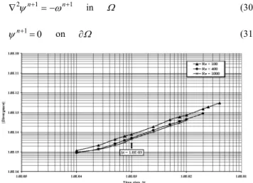
The time accuracy of the method is checked on the steady$state solution of the regularized square driven cavity flow for three values of the Reynolds number, Re = 100, 400 and 1000. To measure the temporal accuracy, the discrete norm of the divergence on the inner
collocation points,∇.V has been considered:
∑ ∑
− = − = ∇ − − = ∇ 1 2 1 2 2 2 )] , ( [ ) 1 )( 1 ( 1 N i M j j i y x .V M N .V (27)Figure 2 shows the variation of the discrete norm of the
divergence on the inner collocation points with the time step
t
forthe steady$state solutions of three values at Re = 100, 400 and 1000 on a grid of Chebyshev of 33x33. In this figure, it can be noticed that as the time step diminishes the discrete norm of the divergence also diminishes (order of accuracy increases). Our numerical
experiments indicate that the critical time step tc(maximal time
step to guarantee the stability of the method) varies with the Reynolds number. Thus, for a Reynolds number of 100 it is
necessary a t≤ 0.04 (Ltc =0.04) for stability of the scheme,
while that, for a Reynolds number of 1000 a value of
01
0
.
t
≤
(L
t
c=
0
.
01
)
is required for the scheme to becomestable. Then, the choice of a time step of 0.001 is enough to guarantee the stability of the method as well as a high precision for all the Reynolds numbers to be studied.
To study the convergence of the solution with respect to the
spatial resolution, the stream function
ψ
and the vorticityω
associated with the regularized cavity flow has been considered.
Thus, at each time step, the vorticity
ω
is computed according toy u x
vn n
n ∂ ∂ − ∂ ∂ = + +
+1 1 1
ω (28)
and the steady$state solution is reached when
,... 2 , 1 , 0 , 10 2 max max 8 1 2 1 2 1 , , 1 2 1 2 , 1 , , = < − − − = − = + − = − = +
∑ ∑
∑ ∑
n x t N i M j n j i j i N i M j n j i n j i j i ω ω ω (29)The streamfunctionψ is computed using the following Poisson
equation
1 1 2 + =− +
∇ψn ωn in (30)
0 1=
+
n
ψ on ∂ (31)
Figure 2. Variation of the discrete norm of the divergence with the time step 4t on a grid of Chebyshev of 33x33.
The convergence is assessed by considering the steady$state regularized driven cavity flow for two values of Re = 100 and 400. The comparisons of some characteristic flow variables are made with those of Botella (1997), who used a third$order time accurate Chebyshev projection scheme for approximating the Navier$Stokes incompressible equations, and Ehrenstein and Peyret (1989), who used a Chebyshev collocation method for solving the Navier$Stokes equations based upon a vorticity$stream function formulation. The comparisons were carried out for different spatial resolutions on the
maximal value of the streamfunction ψ on the inner collocation
points and the maximal value of the vorticity ω on the moving top
side(x,1):
) ( max 1 xi,yj
M = ψ on the inner collocation points;
) 1 , ( max
2 xi
M = ω on the collocation points of the upper side
1 = y . ) , x (
M3=maxω 1 from solution interpolated on 201 equally
Tables 1 and 2, respectively, display these comparisons. For
Re = 100, the results of the present method for M1 and M2 are in
good agreement with the results obtained by Botella (1997) and also
by Ehrenstein and Peyret (1989) for a grid N=M>17. For Re =
400, the values of M1 and M2 obtained by the present method
agree well with those results obtained by Botella (1997) and by
Ehrenstein and Peyret (1989) for a grid N=M >21. The evolution
of M1and M2, when the spatial resolution N increases, is not the
best indication of convergence of the solution. The sensitive
quantity such as M2 does not give a precise account of the maximal
value of the vorticity
ω
, because of the strong variation of thevorticity on the moving top side
ω
(
x
,
1
)
, and the unequaldistribution of the Chebyshev$Gauss$Lobatto points. So, it is much more significant to consider the maximal value of the polynomial
) , x (
N 1
ω on x∈[−1,1]. From the knowledge of the grid values
N ,.., , i ), , x
( i1 =1 2
ω , the continuous polynomial ωN(x,1) is
reconstructed through the Chebyshev expansion (Eq. 19) after having calculated the Chebyshev coefficient with Eq. (22). Thus, the
maximal value of the polynomial ωN(x,1) taken on 201 equally
spaced points on the moving top side is denoted by M3 (Peyret,
2002).
The evolution of the quantity M3, when N increases, provides
a monotonic convergence of the numerical solution. For a
sufficient number of collocation points, the present method converges for very near values to those obtained by Botella (1997) and Ehrenstein and Peyret (1989) (see Table 1 and 2). Thus, for
Re = 100 and 400, the values de M3 obtained by the present
method for N=33 (M3 = 13.4443 and M3 = 24.9110) and
41
=
N (M3 = 13.4444 and M3 = 24.9109) show that 33
collocation points are sufficient to represent correctly a regularized
Table 1. Comparison of the characteristic flow variablesM1,M2,M3for the regularized square driven cavity at Re = 100.
M
N= M1 M1
& '())*+
2
M M2
& '())*+
2
M
, '()-)+
3
M M3
& '())*+
3
M
, '()-)+
17 8.3115E$02 8.3160E$02 13.3347 13.3467 13.3687 13.4628 13.4476 13.4663
21 8.2673E$02 8.2694E$02 13.1869 13.1759 13.1780 13.4472 13.4441 13.4459
25 8.3306E$02 8.3315E$02 13.4291 13.4226 13.4227 13.4449 13.4446 13.4446
33 8.3400E$02 8.3402E$02 13.3441 13.3423 13.3422 13.4443 13.4448 13.4447
41 8.3595E$02 $ 13.4430 $ $ 13.4444 13.4447 $
Table 2. Comparison of the characteristic flow variablesM1,M2,M3 for the regularized square driven cavity at Re = 400.
M
N= M1 M1
& '())*+
2
M M2
& '())*+
2
M
, '()-)+
3
M M3
& '())*+
3
M
, '()-)+
17 8.5341E$02 8.5777E$02 24.7189 24.7799 25.2329 25.0855 25.1604 25.4675
21 8.5113E$02 8.5192E$02 24.6189 24.6268 24.6693 24.9362 24.9273 24.9846
25 8.5671E$02 8.5716E$02 24.9172 24.9157 24.9344 24.9176 24.9148 24.9333
33 8.5467E$02 8.5480E$02 24.7821 24.7845 24.7845 24.9110 24.9111 24.9110
41 8.5893E$02 $ 24.8622 $ $ 24.9108 24.9109 $
cavity flow, the relative difference between M3 obtained for
33
=
N and for N=41 is less than 8E$06. This relative difference
is the same for the values de M3obtained by Botella (1997).
Then, to represent well the steady$state flow with the vortices inside of the regularized cavity for all the numbers of Reynolds a mesh of 33x33 was used in combination with a time step fixed of 0.001 to guarantee a high precision and stability of the present method as well as avoiding high computational cost.
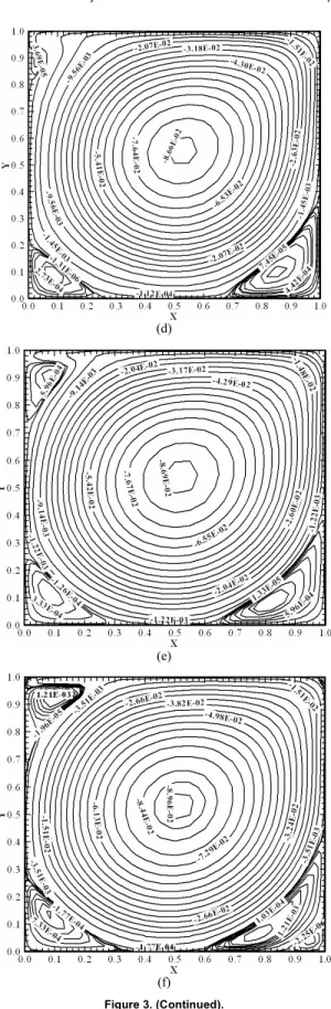
The flow configuration is characterized by the magnitude and the location of the centers of the primary and secondary vortices. The steady state streamfunction contours were computed solving the equation of Poisson (Eqs. (30) $ (31)). The center of the primary vortex was defined using the criterion of the location of the minimum value of the streamfunction. The centers of the secondary vortices were defined using the criterion of the location of the maximum value of the streamfunction and the centers of the vortices tertiary were defined using the criterion of the location of the minimum value of the streamfunction.
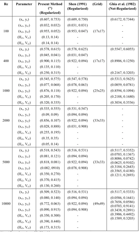
Table 3 shows the comparison of the some characteristic values of the regularized square driven cavity flow with previously
published numerical results obtained by Shen (1991), according to the nomenclature in Fig. 1b. Shen (1991) used the projection scheme of Kim and Moin (1985) in conjunction with a Chebyshev$ Tau space discretization. Shen (1991) results were based on uniform grids of 17x17 up to 49x49 depending on the Reynolds numbers (see Table 3). Although we have used only a 33x33 grid for all cases, the solutions are in good agreement.
The numerical results obtained by Ghia et al. (1982) for the driven cavity flow (not$regularized) for Reynolds numbers up to 10000 are also shown in the Table 3. Ghia et al. (1982) used the vorticity$streamfunction formulation of incompressible Navier$ Stokes equations and a multigrid method, with a 129x129 uniform mesh at Re = 1000 and a 257x257 uniform mesh at Re ≥ 5000.
The comparison of the some characteristic values of the regularized driven cavity flow with numerical results obtained by Ghia et al. (1982) shows that the vortex dynamics between the two cavity flows (regularized and not$regularized) is very similar although the quantitative characteristics are somewhat different.
and location of the centers of the primary and secondary vortices with Reynolds numbers. The some streamfunction contour values for all Reynolds number are shown in theses Figures.
In the Figs. 3a, 3b and 3c can also be observed the formation and growing of the secondary vortices at the bottom left and bottom right of the cavity when the Reynolds number increases. These figures show mainly that the secondary vortices for the Reynolds numbers studied can be very well represented using only 33x33 points of collocation, thanks to the condensed distribution of the Chebyshev$Gauss$Lobatto points near the boundary.
Figures 3d, 3e and 3f show the streamlines of the steady flow for three Reynolds numbers (Re = 2000, 5000 and 10000). Once again, can be observed the formation, evolution and growing of another secondary vortex that appears at the top left of the regularized cavity. At Re = 10000, a tertiary vortex becomes visible at the bottom right of the cavity with center in (0.945, 0.04) and another small tertiary vortex begins to appear at the top right corner (see Fig. 3f). These figures show than the secondary and tertiary vortices for Reynolds numbers up 10000 can be very well represented with only 33x33 points of Chebyshev collocation.
Table 3. Comparison of some characteristic values of the regularized square driven cavity flow.
#
'.+ '# " +
'())(+ '# " +
' + / '()-0+
' 1# " +
100
(xc, yc)
(xs1, ys1)
(xs2, ys2)
(Hs1, Vs1)
(Hs2, Vs2)
(0.607, 0.753)
(0.032, 0.032)
(0.955, 0.052)
(0.13, 0.14)
(0.14, 0.14)
(0.609, 0.750)
(0.031, 0.031)
(0.953, 0.047)
$
$
(17x17)
(0.6172, 0.7344)
$
$
$
$
400
(xc, yc)
(xs1, ys1)
(xs2, ys2)
(Hs1, Vs1)
(Hs2, Vs2)
(0.578, 0.615)
(0.045, 0.041)
(0.900, 0.115)
(0.135, 0.110)
(0.250, 0.315)
(0.578, 0.625)
(0.031, 0.047)
(0.922, 0.094)
$
$
(17x17)
(0.5547, 0.6055)
(0.8906, 0.1250)
(0.2167, 0.3203)
1000
(xc, yc)
(xs1, ys1)
(xs2, ys2)
(Hs1, Vs1)
(Hs2, Vs2)
(0.545, 0.575)
(0.077, 0.068)
(0.876, 0.118)
(0.205, 0.170)
(0.320, 0.335)
(0.547, 0.578)
(0.078, 0.063)
(0.922, 0.094)
$
$
(25x25)
(0.5313, 0.5625)
(0.0859, 0.0781)
(0.8594, 0.1094)
(0.2188, 0.1680)
(0.3034, 0.3536)
2000
(xc, yc)
(xs1, ys1)
(xs2, ys2)
(xs3, ys3)
(Hs1, Vs1)
(Hs2, Vs2)
(Hs3, Vs3)
(0.535, 0.555)
(0.09, 0.09)
(0.856, 0.107)
(0.028, 0.888)
(0.255, 0.195)
(0.35, 0.35)
(0.05, 0.14)
(0.531, 0.547)
(0.094, 0.094)
(0.922, 0.094)
(0.031, 0.908)
$
$
$
(33x33)
$
$
$
$
$
$
$
5000
(xc, yc)
(xs1, ys1)
(xs2, ys2)
(xs3, ys3)
(Hs1, Vs1)
(Hs2, Vs2)
(Hs3, Vs3)
(0.518, 0.543)
(0.081, 0.121)
(0.818, 0.081)
(0.082, 0910)
(0.350, 0.270)
(0.370, 0.415)
(0.130, 0.260)
(0.516, 0.531)
(0.094, 0.094)
(0.922, 0.094)
(0.078, 0.908)
$
$
$
(33x33)
(0.5117, 0.5352) (0.0703, 0.1367) (0.8086, 0.0742) (0.0625, 0.9102) (0.3184, 0.2643) (0.3565, 0.4180) (0.1211, 0.2693)
10000
(xc, yc)
(xs1, ys1)
(xs2, ys2)
(xs3, ys3)
(Hs1, Vs1)
(Hs2, Vs2)
(Hs3, Vs3)
(0.509, 0.523)
(0.080, 0.140)
(0.772, 0.063)
(0.090, 0.915)
(0.350, 0.300)
(0.390, 0.440)
(0.173, 0.315)
(0.516, 0.531)
(0.094, 0.094)
(0.922, 0.094)
(0.094, 0.908)
$
$
$
(49x49)
(0.5117, 0.5333)
(0.0586, 0.1641) (0.7656, 0.0586) (0.0703, 0.9141) (0.3438, 0.2891) (0.3906, 0.4492) (0.1589, 0.3203)
(*) – All results using a 33x33 grid
Shen (1991) found a stationary solution up to Re = 10000. He found that the first Hopf bifurcation (when the steady flow loses its
computed solution loses the time periodicity and becomes quasi$ periodic, which indicated that another bifurcation occurs at a critical Reynolds number between 15000<Re<16000. Botella (1997) used a third$order time accurate Chebyshev projection scheme to compute the flow at Re = 10300, starting from steady solution at Re = 10000 and the flow reached a periodic state.
In our study, we found that the flow converges to steady state for Reynolds numbers up to 10000 and our numerical results did not show any evidence of a Hopf bifurcation, in agreement with the
(a)
(b)
(c)
Figure 3. Steady state streamlines of the regularized square driven cavity flow: (a) Re = 100, (b) Re = 400, (c) Re = 1000, (d) Re = 2000, (e) Re = 5000, (f) Re = 10000.
(d)
(e)
(f)
Figure 3. (Continued).
results obtained by Shen (1991) and Botella (1997).
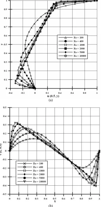
Finally, the u and v velocity component profiles along the
(a)
(b)
Figure 4. Variation of the velocity profiles on the centerline of the regularized driven cavity for some Reynolds numbers: (a) u9velocity, (b)
v9velocity.
% & % 1
The steady viscous incompressible flow over a backward$facing step is a benchmark problem that has been studied by numerous authors using a wide variety of numerical methods. Consider the area containing a step, as shown in Fig. 5. The channel is defined to
have an unitary height H with a step height localized in the
upstream inlet region equal to H/2 and the downstream channel
length is L=25H. The coordinate system to describe the locations
in the channel is centered at the step corner. The definition of the problem as well as the nomenclature used follows Gartling (1990).
Figure 5. Geometry of the backward9facing step and boundary conditions.
The boundary conditions for the channel geometry are the no$ slip conditions for all walls. The inlet velocity field is specified as a parallel flow with a parabolic horizontal component defined by;
) y . ( y ) y (
u =24 05− for 0≤y≤0.5 (32)
This parabolic profile produces a maximum inflow velocity of
5
1
max.
u
=
and an average inflow velocity uavg =1.0. The outflowboundary condition used is a velocity field obtained from the parabolized Navier$Stokes incompressible equations and a Buffer zone is placed at the end of the channel (see Fig. 5). The Reynolds number is defined by the following relation:
ν H/ u
Re= avg (33)
A Buffer zone technique (Streett and Macaraeg, 1989/90) is implemented on a single domain. This technique recognizes the fact that the source of possible reflections from the outflow boundary is the elliptic nature of the Navier$Stokes equations arising from the viscous diffusion terms and from the pressure field. The idea is to remove this ellipticity at the outflow boundary. Then, the first source of ellipticity; the normal viscous terms are smoothly reduced
to zero at the outflow boundary multiplying by a filter function sj.
Similarly, the ability of the pressure field to carry signals back into the domain from the outer boundary is attenuated to zero at outflow by multiplying the source term of the pressure Poisson equation by the filter function. In the present simulations, the filter function utilized is a general function very similar to that used by Joslin et.al. (1991) which is expressed as
(
)
(
)
− − − +
=
b x
b j
N N
N j tanh
s 1 41 2
2
1 (34)
where Nb is the number of the point that marks the beginning of the
Buffer zone and Nx is the number of the point that marks the
position of the outflow boundary.
All numerical simulations for the backward$facing step flow
were computed using a dimensionless channel length of 25H, an
appropriate grid of 91x41 points of Chebyshev collocations. The Buffer zone was set on point 79 of the grid (using 12 points of collocation in this zone) and the time step used in all simulations was 0.005 to guarantee the stability of the present method.
the comparison of the positions of the separation and reattachments points shows good agreement.
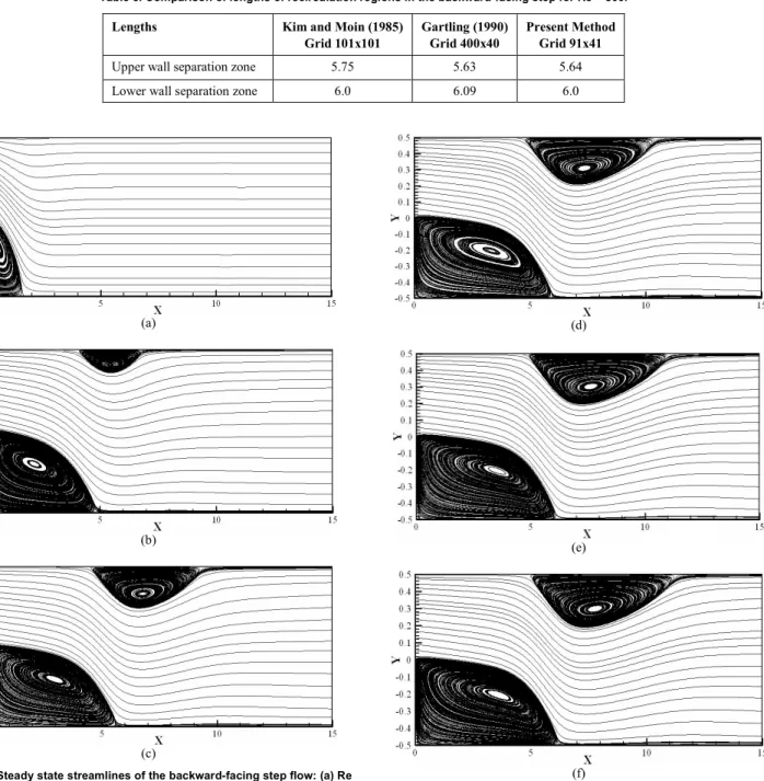
Table 5 shows the comparison of lengths of recirculation regions in the backward$facing step for Reynolds number of 800
with numerical results obtained by others authors. The comparison of the present results shows good agreement with results of Kim and Moin (1985) and Gartling (1990). Kim and Moin (1985) used a finite difference method with a grid of 101x101.
Table 4. Comparison of some characteristic values of the backward9facing step for Re = 800.
2 3 4 " '35 + '())6+
766376 )(37(
Top vortex Separation point
Reattachment point
(4.85, 0.50) (10.48, 0.50)
(4.81, 0.50) (10.45, 0.50)
Bottom vortex Separation point Reattachment point
(0.00, 0.00) (6.09, 0.00)
(0.00, 0.00) (6.00, 0.00)
Table 5. Comparison of lengths of recirculation regions in the backward9facing step for Re = 800.
4 8 '()-9+
(6(3(6(
'())6+
766376 )(37(
Upper wall separation zone 5.75 5.63 5.64
Lower wall separation zone 6.0 6.09 6.0
(a)
(b)
(c)
Figure 6. Steady state streamlines of the backward9facing step flow: (a) Re = 100, (b) Re = 500, (c) Re = 700, (d) Re = 800, (e) Re = 850, (f) Re = 875 (Martinez, 2005).
(d)
(e)
(f)
Figures 6a $ 6f show the steady state streamlines of the backward$facing step flow for Reynolds numbers up to 875. Note
that these figures only show the first 30 step heights(H/2) of the
channel(x=30(H /2)=15).
In these figures, it can be observed the formation and growth of the vortices that appear at the top and bottom of the backward$ facing step when the Reynolds number increases. For example, for Reynolds numbers of 800 the flow separates at the step corner and
forms a large recirculation eddy (Bottom vortex) with a
reattachment point on the lower wall positioned approximately 12
step heights downstream(x≈6). A second recirculation eddy (Top
vortex) forms on the upper wall beginning approximately 10 step
heights downstream(x≈5) and finishing approximately at 21 step
heights downstream(x≈10.5). The figures show that the vortices
for these Reynolds numbers (Re = 100, 500, 700, 800, 850 and 875) can be very well represented using a coarse grid of 91x41 collocation points of Chebyshev.
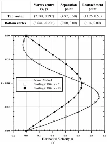
Table 6 shows some characteristic values of the two separation zones that occur in the backward$facing step for Reynolds number of 875.
Table 6. Some characteristic values of the separation zones of the backward9facing step for Re = 875.
2 3
'35 +
#
3 (7.748, 0.297) (4.97, 0.50) (11.26, 0.50)
& 3 (3.644, $0.206) (0.00, 0.00) (6.14, 0.00)
(a)
Figure 7.u9velocity component profiles across the channel at x=7 and
15
x= : (a) Re = 800, (b) Re = 875.
(b)
Figure 7. (Continued).
Figure 7a shows the comparison of
u
velocity componentprofiles across the channel located at x=7 (14 step heights
downstream of the step) and x=15 (30 step heights downstream
of the step) for Reynolds number of 800 with numerical results obtained by Gartling (1990). Here it can be observed the good agreement between velocity profiles obtained by the present method
and those obtained by Gartling (1990). The variation of
u
velocitycomponent profiles across the channel located at x=7and x=15
for Reynolds number of 875 is also shown in the Fig. 7b.
Finally, the comparison of vorticity profiles across the channel
located at x=7 and x=15 for Reynolds number of 800 is shown
in the Fig. 8a. Once again, can be noted the good agreement
between vorticity profiles obtained by the present method and
those obtained by Gartling (1990). Figure 8b shows the variation of
vorticity profiles across the channel located at x=7 and x=15
for Reynolds number of 875.
(a)
(b)
Figure 8. (Continued).
$
The projection method combined with the Chebyshev
collocation spectral method associated with a second order explicit$ implicit time scheme and appropriate boundary conditions, has shown to be a very stable scheme when applied to the solution of the Navier$Stokes equations for two$dimensional incompressible flow.
This combination of the projection scheme in conjunction with a Chebyshev collocation spectral method has been able to predict very well the behavior of the recirculating zones of the two$dimensional regularized square driven cavity flow for Reynolds numbers up to 10000 and the separation zones of the steady viscous incompressible flow over a backward$facing step for Reynolds numbers up to 875. A good agreement was obtained from comparison of the numerical results obtained by the present method with available numerical solutions.
: %
This work was sponsored by CAPES.
The calculations were performed on computer PC$Pentium III$ 700 MHz of the Department of Ocean Engineering, Federal University of Rio de Janeiro, COPPE/UFRJ.
# ;
Botella, O., 1997, “On the Solution of the Navier$Stokes Equations using Chebyshev Projection Schemes with Third$Order Accuracy in Time”,
Computers & Fluids, Vol. 26, No. 2, pp. 107$116.
Boyd, J.P., 2001, “Chebyshev and Fourier Spectral Methods”, Ed. Springer$Verlag, Berlin, 688 p.
Brown, D.L., Cortez, R. and Minion, M.L., 2001, “Accurate Projection Methods for the Incompressible Navier$Stokes Equations”, Journal of Computational Physics, Vol. 168, pp. 464$499.
Canuto, C., Hussaini, M., Quarteroni, A. and Zang, T.A., 2006, “Spectral Methods. Fundamentals in Single Domains”, Ed. Springer$Verlag, Berlin, 585 p.
Chen, H., Su, Y. and Shizgal, B.D., 2000, “A Direct Spectral Collocation Poisson Solver in Polar and Cylindrical Coordinates”,Journal of Computational Physics, Vol. 160, pp. 453$469.
Chorin, A.J., 1968, “Numerical Solution of the Navier$Stokes Equations”,Mathematics of Computation, Vol. 22, pp. 745$762.
Deville, M., Fischer, P.F. and Mund, E.H., 2002, “High$Order Methods for Incompressible Fluid Flow”, Cambridge Monographs on Applied and Computational Mathematics. Cambridge University Press, 499 p.
Ehrenstein, U. & Peyret, R., 1989, “A Chebyshev Spectral Collocation Method for the Navier$Stokes Equations with Application to Double$ Diffusive Convection”, International Journal for Numerical Methods in Fluids, Vol. 9, pp. 427$452.
Gartling, D.K., 1990, “A Test Problem for Outflow Boundary Conditions$Flow over a Backward$Facing Step”,International Journal for Numerical Methods in Fluids, Vol. 11, pp. 953$967.
Ghia, U., Ghia, K.N. and Shin, C.T., 1982, “High$Re Solutions for Incompressible Flow using the Navier$Stokes Equations and a Multigrid Method”,Journal of Computational Physics, Vol. 48, pp. 387$411.
Huges, S. & Randriamampianina, A., 1998, “An Improved Projection Scheme Applied to Pseudospectral Methods for the Incompressible Navier$ Stokes Equations”,International Journal for Numerical Methods in Fluids, Vol. 28, pp. 501$521.
Joslin, R.D., Streett, C.L. and Chang, C.L., 1991, “Validation of 3D Incompressible Spatial Direct Numerical Simulation Code. A Comparison with Linear Stability and Parabolic Stability Equation Theories for Boundary Layer Transition on a Flat Plate”, Report NASA Langley Research Center, NASA TP$3205, pp$1$47.
Kim, J. & Moin, P., 1985, “Application of a Fractional$Step Method to Incompressible Navier$Stokes Equations”, Journal of Computational Physics, Vol. 59, pp. 308$323.
Lynch, R.E., Rice, J.R. and Thomas, D.H., 1964, “Direct Solution of Partial Differential Equations by Tensor Product Matrices”, Numerical Mathematics, Vol. 6, pp. 185$199.
Martinez, J.J., 1999, “Application of the Chebyshev Pseudospectral Method on some Hydrodynamic Problems” (In Portuguese), M.Sc. Thesis, Federal University of Rio de Janeiro, Rio de Janeiro, RJ, Brazil, 141 p.
Martinez, J.J., 2005, “Application of Spectral Multidomain Method for Simulation of Incompressible Viscous Flows” (In Portuguese), Ph.D. Thesis, Federal University of Rio de Janeiro, Rio de Janeiro, RJ, Brazil, 149 p.
Peyret, R., 2002, “Spectral Methods for Incompressible Viscous Flow”,
Applied Mathematical Sciences, Vol. 148, Ed. Springer$Verlag, New York, 448 p.
Shankar, P.N. & Deshpande, M.D., 2000, “Fluid Mechanics in the Driven Cavity”,Annual Review of Fluid Mechanics, Vol.32, pp. 93$136.
Shen, J., 1991, “Hopf Bifurcation of the Unsteady Regularized Driven Cavity Flow”,Journal of Computational Physics, Vol. 95, pp. 228$245.
Streett, C.L. & Macaraeg, M.G., 1989/90, “Spectral Multi$Domain for Large$Scale Fluid Dynamic Simulations”,Applied Numerical Mathematics, Vol. 6, pp. 123$139.
Solomonoff, A. & Turkel, E., 1989, “Global Properties of Pseudospectral Methods”,Journal of Computational Physics, Vol. 81, pp. 239$276.
Tanahashi, T. & Okanaga, H., 1990, “GSMAC Finite Element Method for Unsteady Incompressible Navier$Stokes Equations at High Reynolds Numbers”,International Journal for Numerical Methods in Fluids, Vol.11, pp. 479$499.
Temam, R., 1968, “Une Méthode d’Approximation de la Solution des Équations de Navier$Stokes”,Bulletin of Society Mathematics of France, Vol. 98, pp. 115$152.
Trefethen, L.N., 2000, “Spectral Methods in Matlab”, SIAM, University City Science Center, Philadelphia, USA, 165 p.