Application of spectral collocation method to a class of nonlinear PDEs

(1)

Available online at www.ispacs.com/cna Volume 2013, Year 2013 Article ID cna-00136, 14 Pages

doi:10.5899/2013/cna-00136 Research Article

Application of spectral collocation method to a class of

nonlinear PDEs

M. Zarebnia1∗_{, S. Jalili}1

(1)Department of Mathematics, University of Mohaghegh Ardabili, 56199-11367, Ardabil, Iran

Copyright 2013 c⃝M. Zarebnia and S. Jalili. This is an open access article distributed under the Creative Commons Attribution License, which permits unrestricted use, distribution, and reproduction in any medium, provided the original work is properly cited.

Abstract

In this paper approximate solutions to a class of nonlinear partial differential equations by means of the Chebyshev spectral collocation method is considered. First, properties of the Chebyshev spectral collocation method required for our subsequent development are given and utilized to reduce the computation of Fisher’s, generalized Burger’s-Fisher, generalized Huxley, and generalized Burger’s-Huxley equations to some system of ordinary differential equations. Then, we use fourth-order Runge-Kutta formula for the numerical solution of the system of ordinary differential equations. The method is applied to a few test examples to illustrate the accuracy and the implementation of the method.

Keywords:Chebyshev; Spectral method; Fisher; Generalized Burger-Fisher; Generalized Huxley; Generalized Burger-Huxley.

1 Introduction

In this paper a Chebyshev spectral collocation method is used for the numerical solution of the following nonlinear partial differential equations:

I) Fisher’s equation [1, 2]

ut=uxx+u(u−1), (x,t)∈D×[0,T], (1.1)

II) generalized Burger’s-Fisher equation [3, 4]

ut+αuδux−uxx=βu(1−uδ), (x,t)∈D×[0,T], (1.2)

whereα,β, andδ are parameters, III) generalized Huxley equation [5, 6]

ut−uxx=βu(1−uδ)(uδ−γ), (x,t)∈D×[0,T], (1.3)

whereδ,β≥0 andγ∈(0,1)are given parameters,

IV) generalized Burger’s-Huxley equation [7, 8]

ut+αuδux−uxx=βu(1−uδ)(uδ−γ), (x,t)∈D×[0,T], (1.4)

(2)

whereα,β,γ andδ are parameters,β≥0,δ >0,γ∈(0,1).

For the problems (1.1)-(1.4), we consider initial condition

u(x,0) =f(x), x_∈D, (1.5) and boundary conditions

u(x,t) =g(t), (x,t)∈∂D_×[0,T], (1.6) whereD={x:a<x<b_}and∂Dis its boundary.

Nonlinear phenomena are of fundamental importance in various fields of science and engineering. Non-linear partial differential equations (1.1)-(1.4) play important roles in non-linear physics [9]-[17]. The Fishers equation is first intro-duced by Fisher as a deterministic model of the wave propagation of favored gene in population [9]. Also, the Fisher’s equation arises in many physical, biological, chemical, and engineering problems that are described by the interaction of diffusion and reaction process. For example, it plays a significant role include flame propagation, neutron flux in a nuclear reactor and the dynamics of defects in nematic liquid crystal [10]. Burger’s equation arises in many physi-cal problems including one dimensional turbulence, gas dynamics, number theory, heat conduction, elasticity, sound waves in viscous medium [11], shock waves in viscous medium, waves in a medium with fluid filled viscoelastic tubes and magnetohydrodynamic waves in a medium with finite electrical conductivity. The core mathematical framework for modern biophysically based neural modeling was developed half a century ago by Hodgkin and Huxley [12]. In a series of papers published in 1952, they presented the results of an elegant series of electrophysiological experiments in which they investigated the flow of electric current through the surface membrane of the giant nerve fiber of a squid. The Burger’s-Huxley equation describes the interaction between diffusion, convection and reaction.

The layout of the paper is as follows. First, in Section 2 we review some of the main properties of Chebyshev polynomials that are necessary for the formulation of the discrete system. In Section 3, we illustrate how the Cheby-shev spectral collocation method may be used to replace Eqs. (1.1)-(1.6) by explicit system of ordinary differential equations, which is solved by fourth-order Runge-Kutta method. In Section 4, we report our numerical results and demonstrate the efficiency and accuracy of the proposed numerical scheme by considering some numerical examples.

2 Preliminaries

The goal of this section is to recall notations and definition of the Chebyshev polynimials, state some known results, and derive useful formulas that are important for this paper. These are discussed thoroughly in [18].

The well known Chebyshev polynomialTn(x)of the first kind is a polynomial inxof degree n, defined by the relation

Tn(x) =cosnθ when x=cosθ. (2.7) If the range of the variablexis the interval [-1,1], then the range of the corresponding variableθcan be taken as[0,θ]. These ranges are traversed in opposite directions, sincex=−1 corresponds toθ=πandx=1 corresponds toθ=0. It is well known that cosnθ is a polynomial of degree n in cosθ, and indeed we are familiar with the elementary formulae

cos 0θ=1, cos 1θ=cosθ, cos 2θ=2 cos2θ−1,

cos 3θ=4 cos3θ−3 cosθ, cos 4θ=8 cos4θ−8 cos2θ+1, . . . .

We may immediately deduce from (2.7), that the first few Chebyshev polynomials are

T0(x) =1, T1(x) =x, T2(x) =2x2−1, T3(x) =4x3−3x, T4(x) =8x4−8x2+1, . . . .

In practice it is neither convenient nor efficient to work out eachTn(x)from first principles. Rather by combining the trigonometric identity

(3)

with equation (2.7), we obtain the fundamental recurrence relation

Tn(x) =2xTn−1(x)−Tn−2(x), n=2,3, . . . , (2.8)

which together with the initial conditions

T0(x) =1, T1(x) =x, (2.9) recursively generates all the polynomials{Tn(x)}very efficiently.

Clenshaw and Curtis [19] introduced the following approximation of the functionu(x,t):

u(x,t) = N

∑

j=0

′′_a

jTj∗(x), (2.10)

whereT_j∗(x) =Tj((2x−(b+a))/(b−a))denotes the jthshifted Chebyshev polynomial of the first kind. Note the

double prime indicating that the first and last terms of the sum are to be halved. We can use the discrete orthogonality relation

N

∑

n=0

′′_T∗

i (xn)Tj∗(xn) =αi,j, (2.11)

where

αi,j= 





0, i_̸=j(≤N), 1

2N, 0<i=j<N, N, i=j=0,N,

(2.12)

and also, the collocation pointsxnare given by

xn=

1 2

(

(a+b)−(b₋a)cos(πn

N

))

, n=0,1, . . . ,N. (2.13)

We can invert the interpolating polynomial defined as (2.13) and find

aj=

2 N

N

∑

n=0

′′_T∗

j(xn)u(xn,t). (2.14)

The relation between the Chebyshev functions and the first derivative is given by [20]:

T_j∗′(x) =2jλ j₋1

∑

n=0,n+j odd

cnTn∗(x), (2.15)

whereλ=_b₋2_aand

cn= {

1, 1≤n_≤N₋1, 1

2, n=0,N.

(2.16)

3 The Chebyshev spectral collocation method

(4)

3.1 _{Fisher’s equation}

Let us consider the Fisher’s equation

ut=uxx+u(u−1), (x,t)∈D×[0,T], (3.17)

with the initial condition

u(x,t) =g(t), (x,t)∈∂D_×[0,T], (3.19) whereD={x:a<x<b_}and∂Dis its boundary. We assumeu(x,t)defined over theD_×[0,T]be the exact solution of the problem (3.17)-(3.19) that is approximated as follows:

u(x,t) = N

∑

j=0

′′_a

jTj∗(x). (3.20)

By considering the Equation (3.19) and the Chebyshev coefficientsajthat is defined by (2.14), we can obtain the first

derivative ofu(x,t)at the collocation points (2.13) as follows:

d

dxu(xi,t) =ux(xi,t) =

N

∑

j=0

′′_a jTj∗′(xi)

= N

∑

j=0

′′(2

N

∑

n=0

′′_T∗

j(xn)u(xn,t) )

T_j∗′(xi)

= N

∑

n=0

′′(2

N

∑

j=0

′′_T∗

j′(xi)Tj∗(xn) )

u(xn,t)

= N

∑

n=0

Dx_i_,_nu(xn,t), (3.21)

where

Dx_i_,_n=2cn

N

∑

j=0

′′_T∗

j′(xi)Tj∗(xn), i,n=0,1, . . . ,N−1,N, (3.22)

and also,T_j∗′(xi)andcnare defined by (2.15) and (2.16) respectively.

Having used the boundary conditions (3.19), we rewrite the Eq. (3.21) as follows:

ux(xi,t) = N

∑

n=0

Dx_i_,_nu(xn,t) =Dxi,0u(x0,t) +

N₋1

∑

n=1

Dx_i_,_nu(xn,t) +Dxi,Nu(xN,t). (3.23)

For the sake of simplicity, consider:

Fi(t) =Dx_i_,₀u(x0,t) +Dxi,Nu(xN,t),

thus we can write:

ux(xi,t) =Fi(t) + N−1

∑

n=1

(5)

Now for the second derivative ofu(x,t)by similarly manner and using Equation (3.21), we obtain:

d2

dx2u(xi,t) =uxx(xi,t) =

N

∑

n=0 Dx_i_,_n(d

dxu(xn,t)

)

= N

∑

n=0 Dx_i_,_n(

N

∑

j=0

Dx_n_,_ju(xj,t) ) = N

∑

j=0 ( N

∑

n=0

Dx_i_,_nDx_n_,_j)u(xj,t). (3.25)

By assumption

Dxx_i_,_j= N

∑

n=0

Dx_i_,_nDx_n_,_j, i,j=0,1, . . . ,N, (3.26)

we have:

uxx(xi,t) = N

∑

j=0

Dxx_i_,_ju(xj,t). (3.27)

By using the boundary conditions (3.19), we obtain:

uxx(xi,t) = N

∑

j=0

Dxx_i_,_ju(xj,t) =Dxxi,0u(x0,t) +

N−1

∑

n=1

Dxx_i_,_nu(xn,t) +Dxxi,Nu(xN,t). (3.28)

We consider the notationF_i∗(t)as follows:

F_i∗(t) =Dxx_i_,₀u(x0,t) +Dxxi,Nu(xN,t), (3.29)

then we can write:

uxx(xi,t) =Fi∗(t) + N−1

∑

n=1

Dxx_i_,_nu(xn,t). (3.30)

Having replaced the first term on the right-hand side of (3.17) with the Eq. (3.30) and setting collocation points

x=xi,i=0,1, . . . ,Nthat are defined by (2.13), we get the collocation result as

ut(xi,t) =Fi∗(t) + N−1

∑

n=1

Dxx_i_,_nu(xn,t) +u(xi,t) (

u(xi,t)−1 )

, (3.31)

u(xi,0) =f(xi).

We denote

Gi(t,u(t)) =F_i∗(t) + N₋1

∑

n=1

Dxx_i_,_nu(xn,t) +u(xi,t) (

u(xi,t)−1 )

,

u(t) = [u(x1,t),u(x2,t), . . . ,u(xN−1,t)]T, u0= [u(x1,0),u(x2,0), . . . ,u(xN−1,0)]T, du(t) = [ut(x1,t),ut(x2,t), . . . ,ut(xN−1,t)]T, then the system of (3.31) can be given in the matrix form as:

du(t) =G(t,u(t)),

(6)

where

G(t,u(t)) = [G1(t,u(t)),G2(t,u(t)), . . . ,GN−1(t,u(t))]T, P= [f(x1),f(x2), . . . ,f(xN−1)]T.

The above system is a system of ordinary differential equations. Solving this system by the fourth-order Runge-Kutta method, we can obtain an approximation to the solution of (3.17). The fourth-order Runge-Kutta method that is one of the well-known numerical methods for differential equations, can be presented as:

u1=htG (

tn,u(tn) )

,

u2=htG(tn+ht,u(tn+

u1 2 )

) ,

u3=htG(tn+ht,u(tn+

u2 2 )

)

, (3.33)

u4=htG(tn+ht,u(tn+u3)),

u(tn+1) =u(tn) + 1 6

(

u1+2u2+2u3+u4).

3.2 _{Generalized Burger’s-Fisher equation}

In this subsection, we consider the generalized Burger’s-Fisher equation

ut+αuδux−uxx=βu(1−uδ), (x,t)∈D×[0,T], (3.34)

with the initial and boundary conditions (3.18) and (3.19). In Eq. (3.34)α,β, andδ are parameters. By considering approximate solutionu(x,t)as in (2.10) and then settingx=xiwe get:

ut(xi,t) =−αuδ(xi,t)ux(xi,t) +uxx(xi,t) +βu(xi,t)(1−uδ(xi,t)), (3.35)

whereux(xi,t)anduxx(xi,t)are approximated by (3.24) and (3.30) respectively.

Having replaced theux(xi,t)anduxx(xi,t)on the right-hand sides of (3.35) with the Eqs. (3.24) and (3.30), we get:

ut(xi,t) =−αuδ(xi,t) (

Fi(t) + N₋1

∑

n=1

Dx_i_,_nu(xn,t) )

+(F_i∗(t) + N₋1

∑

n=1

Dxx_i_,_nu(xn,t) )

+βu(xi,t)(1−uδ(xi,t)), (3.36)

u(xi,0) = f(xi).

Now by assumption

Gi(t,u(t)) =(

−αuδ(xi,t)Fi(t) +Fi∗(t) )

+βu(xi,t)(1−uδ(xi,t))

+(−αuδ(xi,t) N−1

∑

n=1

Dx_i_,_nu(xn,t) + N−1

∑

n=1

(7)

and also

u(t) = [u(x1,t),u(x2,t), . . . ,u(xN−1,t)]T,

u0= [u(x1,0),u(x2,0), . . . ,u(xN₋1,0)]T, (3.37)

du(t) = [ut(x1,t),ut(x2,t), . . . ,ut(xN−1,t)]T, we may rewrite the system (3.36) in the form

du(t) =G(t,u(t)),

u0=P, (3.38)

where

G(t,u(t)) = [G1(t,u(t)),G2(t,u(t)), . . . ,GN−1(t,u(t))]T,

P= [f(x1),f(x2), . . . ,f(xN₋1)]T. (3.39)

Solving system of ordinary differential equations (3.38) by Runge-Kutta method (3.33), we can obtain an approxima-tion to the soluapproxima-tion of (3.34).

3.3 _{Generalized Huxley equation}

In this subsection the chebyshev spectral collocation procedure is developed for the numerical solution of the generalized Huxley equation:

ut−uxx=βu(1−uδ)(uδ−γ), (x,t)∈D×[0,T], (3.40)

with initial condition

u(x,t) =g(t), (x,t)∈∂D_×[0,T], (3.42) whereD={x:a<x<b_},δ,β ≥0 andγ∈(0,1)are given parameters and∂Dis its boundary.

By replacing the second term on the left-hand side of (3.40) with the Eq. (3.30) and setting the collocation points

xi=

1 2

(

(a+b)−(b₋a)cos(πn N

))

, i=0,1, . . . ,N,

we get the collocation result as

ut(xi,t)− (

F_i∗(t) + N₋1

∑

n=1

=βu(xi,t) (

1−uδ(xi,t) )(

uδ(xi,t)−γ )

, (3.43)

whereDxx_i_,_nandF_i∗(t)are defined by (3.26) and (3.29).

Considering the Eqs. (3.37) and (3.39), the system (3.43) can be written in the following form

du(t) =G(t,u(t)),

(8)

where

G(t,u(t)) = [G1(t,u(t)),G2(t,u(t)), . . . ,GN−1(t,u(t))]T, Gi(t,u(t)) =βu(xi,t)(1−uδ(xi,t))(uδ(xi,t)−γ)+Fi∗(t) +

N−1

∑

n=1

Dxx_i_,_nu(xn,t).

Having solved the system (3.44) by the fourth-order Runge-Kutta method, we obtainu(x,t)as (2.10) which is the computed solution for the Huxley equation (3.40).

3.4 _{Generalized Burger’s-Huxley equation}

Finally in this subsection, we illustrate how the spectral collocation method based on the chebyshev polynomial may be used to find approximate solution for the generalized Burger’s-Huxley equation

ut+αuδux−uxx=βu(1−uδ)(uδ−γ), (x,t)∈D×[0,T], (3.45)

with initial and boundary conditions (1.5) and (1.6).α,β,γandδ are parameters,β_≥0,δ>0 andγ_∈(0,1).

We assume the solution

u(x,t) = N

∑

j=0

′′_a

jTj∗(x). (3.46)

be the approximate solution of the problem (3.45).

Similarly, by applying the chebyshev spectral collocation method, using the relations (3.24) and (3.30) and substituting

x=xifori=0, . . . ,N,we obtain the following system

ut(xi,t) =−αuδ(xi,t) (

Fi(t) + N−1

∑

n=1

Dx_i_,_nu(xn,t) )

+(F_i∗(t) + N−1

∑

n=1

+βu(xi,t) (

1−uδ(xi,t) )(

uδ(xi,t)−γ )

,

u(xi,0) =f(xi). (3.47)

By using the notations (3.37) and (3.39), and also,

Gi(t,u(t)) =(−αuδ(xi,t)Fi(t) +Fi∗(t) )

+βu(xi,t)(1−uδ(xi,t))(uδ(xi,t)−γ)

+( N₋1

∑

n=1

Dxx_i_,_nu(xn,t)−αuδ(xi,t) N₋1

∑

n=1

Dx_i_,_nu(xn,t) )

,

u(xi,0) = f(xi),

we then rewrite the system (3.47) in the following form which is the system of ordinary differential equations.

du(t) =G(t,u(t)),

u0=P. (3.48)

(9)

4 Numerical examples

In order to illustrate the performance of the Chebyshev spectral collocation method in solving the problems (1.1)-(1.6) and efficiency of the presented method, the following examples are considered. We assumeuiandu∗i be exact

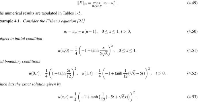
and approximate solutions and use the maximum of absolute error, defined as

∥E_∥∞= max

0<i<N|ui−u ∗

i|, (4.49)

The numerical results are tabulated in Tables 1-5.

Example 4.1. Consider the Fisher’s equation [21]

ut=uxx+u(u−1), 0≤x≤1,t>0, (4.50)

subject to initial condition

u(x,0) =1

4

(

−1+tanh x 2√6

)2

, 0≤x_≤1, (4.51)

and boundary conditions

u(0,t) =1

4

(

1+tanh5t 12

)2

, u(1,t) =1

4

(

−1+tanh 1 12(

√

6−5t) )2

, t>0. (4.52)

which has the exact solution given by

u(x,t) =1

4

(

−1+tanh(1

12(−5t+

√

6x)) )2

. (4.53)

We solve (4.50) for different values of t, ht=10−4. The maximum of absolute errors are tabulated in Table1for

N=4,6,8.

Table 1: The Results for Example 4.1. t N=4 N=6 N=8 0.1 1.9927E-8 1.1487E-11 4.0745E-14 0.15 2.9992E-8 1.9907E-11 4.2410E-14 0.18 3.5647E-8 2.6276E-11 4.9516E-14 0.2 3.9275E-8 3.0459E-11 5.4345E-14 0.25 4.7892E-8 4.0610E-11 6.6058E-14 0.3 5.5879E-8 5.0175E-11 7.7355E-14

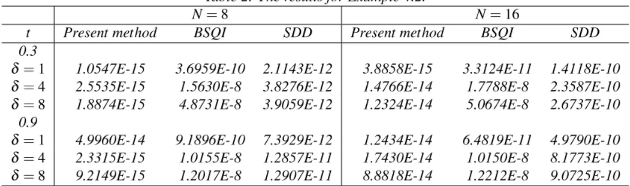
Example 4.2. For the sake of comparison, we consider the following generalized Burger’s-Fisher equation discussed by Zhu et al. [22] and Golbabai et al. [3]. The authors used the cubic B-spline quasi-interpolation (BSQI) and spectral domain decomposition (SDD) methods to obtain their numerical solution.

ut+αuδux−uxx=βu(1−uδ),

u(x,0) = (

1 2−

1 2tanh

( xαδ

2(1+δ) )

)_δ1

u(0,t) = (

1 2+

1 2tanh

(tδ(α2+β(1+δ)2)

2(1+δ)2

) )_δ1

(4.54)

u(1,t) = (

1 2+

1 2tanh

( −αδ

2(1+δ)(1−( α

1+δ +

β(1+δ)

α )t)

(10)

with the exact solution

u(x,t) = (

1 2+

1 2tanh

( −αδ

2(1+δ)(x−( α

1+δ +

β(1+δ)

α )t)

) )_δ1

, (4.55)

whereα,β andδ are arbitrary constants.

We compare the results with the BSQI [22] and SDD [3] applied to same equation. For this purpose, we consider the same parameter values for the generalized Burgers- Fisher equation (4.54) as considered in [3] and [22], namely; N=8, N=16,α=0.1,β=−0.25and ht=10−5. Table 2 exhibits the compared results.

Table 2: The results for Example 4.2.

N=8 N=16

t Present method BSQI SDD Present method BSQI SDD 0.3

δ=1 1.0547E-15 3.6959E-10 2.1143E-12 3.8858E-15 3.3124E-11 1.4118E-10

δ=4 2.5535E-15 1.5630E-8 3.8276E-12 1.4766E-14 1.7788E-8 2.3587E-10

δ=8 1.8874E-15 4.8731E-8 3.9059E-12 1.2324E-14 5.0674E-8 2.6737E-10 0.9

δ=1 4.9960E-14 9.1896E-10 7.3929E-12 1.2434E-14 6.4819E-11 4.9790E-10

δ=4 2.3315E-15 1.0155E-8 1.2857E-11 1.7430E-14 1.0150E-8 8.1773E-10

δ=8 9.2149E-15 1.2017E-8 1.2907E-11 8.8818E-14 1.2212E-8 9.0725E-10

Example 4.3. Consider the generalized Huxley equation [5]

ut−uxx=βu(1−uδ)(uδ−γ), 0≤x≤1, t>0, (4.56)

whereδ, β≥0andγ∈(0,1)are given parameters. The exact solution to Eq. (4.56) is given by

u(x,t) = [_γ

2+

γ

2tanh

{ σ γ

(

x+ρ(1+δ−γ)

2(1+δ) t )}]1_δ

, (4.57)

whereσ=δ ρ/4(1+δ)andρ=2√β(1+δ). The initial and boundary conditions are taken from the exact solutions.

We solve the Example 3 for N=10and ht=10−4. The maximum of absolute errors are tabulated in Table 3 for

the parametersβ=1,δ =1,2,3andγ=0.001.

Table 3: The results for Example 4.3. t δ =1 δ=2 δ =3 0.05 2.3138E-8 1.0348E-6 3.6729E-6

0.1 3.8440E-8 1.7191E-6 6.1019E-6 0.5 4.7799E-8 2.1377E-6 7.5874E-6 0.2 5.3513E-8 2.3932E-6 8.4942E-6 0.25 5.7001E-8 2.5491E-6 9.0476E-6 0.3 5.9131E-8 2.6443E-6 9.3863E-6

(11)

x t Exact present method ADM [5] HPM[6]

0.05 5.00030E-4 5.00020E-4 5.00006E-4 5.00006E-4 0.1 0.1 5.00043E-4 5.00028E-4 4.99993E-4 4.99993E-4 1 5.00268E-4 5.00245E-4 4.99768E-4 4.99768E-4 0.05 5.00101E-4 5.00078E-4 5.00076E-4 5.00076E-4 0.5 0.1 5.00113E-4 5.00075E-4 5.00063E-4 5.00063E-4 1 5.00338E-4 5.00276E-4 4.99839E-4 4.99839E-4 0.05 5.00172E-4 5.00161E-4 5.00147E-4 5.00147E-4 0.9 0.1 5.00184E-4 5.00169E-4 5.00134E-4 5.00134E-4 1 5.00409E-4 5.00380E-4 4.99909E-4 4.99909E-4

Example 4.4. We consider generalized Burger’s-Huxley equation [7]

ut+αuδux−uxx=βu(1−uδ)(uδ−γ), 0≤x≤1, t≥0, (4.58)

with initial condition

u(x,0) =(γ

2+

γ

2tanh(w1x)

)_δ1

, 0≤x_≤1,

and boundary conditions

u(0,t) =(γ

2+

γ

2tanh(−w1w2t)

)_δ1

, t>0,

u(1,t) =(γ

2+

γ

2tanh

(

w1(1−w2t)

)_δ1

, t>0.

The exact solution of Eq. (4.58) is taken from [23], given by

u(x,t) =(γ

2+

γ

2tanh

(

w1(x−w2t)

)1_δ

(4.59)

where

w1=−

αδ+δ√

α2₊₄_β₍₁_+δ₎

2(1+δ) , (4.60)

and

w2=

αγ

1+δ −

(1+δ−γ)(−α+√α2₊₄_β₍₁_+δ₎₎

2(1+δ) , (4.61)

whereα,β,γandδ are constant such thatβ _≥0,δ>0,γ_∈(0,1).

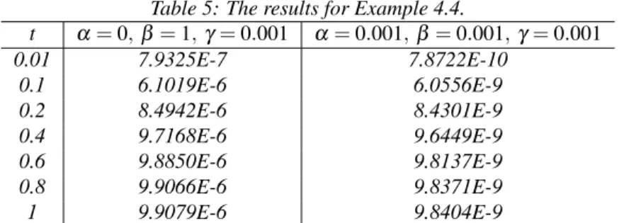
We solved Example 4.4 for different values of t, N=10, ht=10−3andδ=3. The maximum of absolute errors on

the Chebyshev collocation points are tabulated in Table 5 forα=0,β=1,γ=0.001andα=0.001,β=0.001,γ=

(12)

t α=0,β =1,γ=0.001 α=0.001,β=0.001,γ=0.001

0.01 7.9325E-7 7.8722E-10

0.1 6.1019E-6 6.0556E-9

0.2 8.4942E-6 8.4301E-9

0.4 9.7168E-6 9.6449E-9

0.6 9.8850E-6 9.8137E-9

0.8 9.9066E-6 9.8371E-9

1 9.9079E-6 9.8404E-9

5 Conclusion

The Chebyshev spectral collocation method is used to solve the Fisher’s, generalized Burger’s-Fisher, Huxley and generalized Burger’s-Huxley equations with initial and boundary conditions. From the numerical results and Tables 1-5, we can say that errors are very small and they are very better than the results of another papers cited in this article.

6 Acknowledgments

The authors would like to thank the Editor and anonymous reviewers for their valuable comments and suggestions, which were helpful in improving the paper.

References

[1] K. Al-Khaled, Numerical study of Fisher’s reactiondiffusion equation by the sinc collocation method, Journal of Computational and Applied Mathematics, 137 (2001) 245-255.

http://dx.doi.org/10.1016/S0377-0427(01)00356-9

[2] A. M. Wazwaz, A. Gorguis, An analytic study of Fisher’s equation by using Adomian decomposition method, Applied Mathematics and Computation, 154 (2004) 609-620.

http://dx.doi.org/10.1016/S0096-3003(03)00738-0

[3] A. Golbabai, M. Javidi, A spectral domain decomposition approach for the generalized Burger’s-Fisher equation, Chaos, Solitons and Fractals, 39 (2009) 385-392.

http://dx.doi.org/10.1016/j.chaos.2007.04.013

[4] M. Moghimi, F. S. A. Hejazi, Variational iteration method for solving generalized Burger-Fisher and Burger equations, Chaos, Solitons and Fractals, 33 (2007) 1756-1761

[5] I. Hashim, M. S. M. Noorani, B. Batiha, A note on the Adomian decomposition method for the generalized Huxley equation, Applied Mathematics and Computation, 181 (2006) 1439-1445.

http://dx.doi.org/10.1016/j.amc.2006.03.011

[6] S. H. Hashemi, H. R. Mohammadi Daniali, D. D. Ganji, Numerical simulation of the generalized Huxley equa-tion by He’s homotopy perturbaequa-tion method, Applied Mathematics and Computaequa-tion, 192 (2007) 157-161. http://dx.doi.org/10.1016/j.amc.2007.02.128

[7] A. J. Khattak, A computational meshless method for the generalized Burger’s-Huxley equation, Applied Math-ematical Modelling, 33 (2009) 3718-3729.

(13)

[8] M. Javidi, A. Golbabai, A new domain decomposition algorithm for generalized Burger’s-Huxley equation based on Chebyshev polynomials and preconditioning, Chaos, Solitons and Fractals, 39 (2009) 849-857.

[9] R. A. Fisher, The wave of advance of advantageous Genes, Ann. Eugen, 7 (1936) 355-369.

[10] L. Debnath, Nonlinear Partial Differential Equations for Scientists and Engineers, Birkhauser, Boston, 1997.

[11] M. J. Lighthill, Viscosity effects in sound waves of finite amplitude, in: G.K. Batchelor, R.M. Davies (Eds.), Surveys in Mechanics, Cambridge University Press, Cambridge, (1956) 250-351.

[12] A. L. Hodgkin, A. F. Huxley, A quantitative description of membrane current and its application to conduction and excitation in nerve, The Journal of Physiology, 117 (1952) 500-544.

[13] L. X. Duan, Q. S. Lu, Bursting oscillations near codimension-two bifurcations in the Chay Neuron model, Int. J. Nonlinear Sci. Numer. Simul, 7 (2006) 59-64.

http://dx.doi.org/10.1515/IJNSNS.2006.7.1.59

[14] S. Q. Liu, T. Fan, Q. S. Lu, The spike order of the winnerless competition (WLC) models and its application to the inhibition neural system, Int. J. Nonlinear Sci. Numer. Simul, 6 (2005) 133-138.

http://dx.doi.org/10.1515/IJNSNS.2005.6.2.133

[15] D. G. Aronson, H. F. Weinberger, Multidimensional nonlinear diffusion arising in population genetics, Adv. Math, 30 (1978) 33-76.

http://dx.doi.org/10.1016/0001-8708(78)90130-5

[16] G. J. Zhang, J. X. Xu, H. Yao, R. X. Wei, Mechanism of bifurcation-dependent coherence resonance of an excitable neuron model, Int. J. Nonlinear. Sci. Numer. Simul, 7 (2006) 447-450.

[17] H. Panahipour, Application of Extended Tanh Method to Generalized Burgers-type Equations, Communications in Numerical Analysis, 2012 (2012) 1-14.

http://dx.doi.org/10.5899/2012/cna-00058

[18] J. C. Mason, D. C. Hndscomb, Chebyshev Polynomials, Chapman and Hall /CRC, (2003).

[19] C. W. Clenshaw, A. R. Curtis, A method for numerical integration on an antomatic computer, Numer. Math, 2 (1960) 197-205.

http://dx.doi.org/10.1007/BF01386223

[20] E. M. E. Elbarbary, M. El-Kady, Chebyshev finite difference approximation for the boundary value problems, Applied Mathematics and Computation, 139 (2003) 513-523.

http://dx.doi.org/10.1016/S0096-3003(02)00214-X

[21] G. Hariharan, K. Kannan, K. R. Sharma, Haar wavelet method for solving Fisher’s equation, Applied Mathe-matics and Computation, 211 (2009) 284-292.

http://dx.doi.org/10.1016/j.amc.2008.12.089

[22] Ch. G. Zhu, W. Sh. Kang, Numerical solution of Burger’s-Fisher equation by cubic B-spline quasi- interpolation, Applied Mathematics and Computation, 216 (2010) 2679-2686.

(14)

[23] X. Y. Wang, Z. S. Zhu, Y. K. Lu, Solitary wave solutions of the generalized Burger’s-Huxley equation, J. Phys. A: Math. Gen, 23 (1990) 271-274.