Modification of Haessler’s sequential heuristic procedure for the one-dimensional cutting stock problem with setup cost

Production, 28, e20170105, 2018 DOI: 10.1590/0103-6513.20170105 ISSN 1980-5411 (On-line version)

Research Article

This is an Open Access article distributed under the terms of the Creative Commons Attribution License, which

1. Introduction

Paper and steel industries store large amounts of raw material to be cut to manufacture products, because (i) the cost of transport, storage, and handling of large objects is smaller than the cost of the items, when they are considered separately throughout the manufacturing process, and (ii) the uncertainty of the demand for items. The determination of how the stored master rolls (objects) are supposed to be cut to manufacture the reels (items) required by the customers is known as the One-Dimensional Cutting Stock Problem. This classic problem in Operational Research represents a key process in these production chains. To minimize the trim loss or the number of rolls is a straightforward strategy. The first approach in this field was carried out by Kantorovich (1960) – and followed by Metzger (1958), Eilon (1960) and others. However, it was Gilmore and Gomory’s approach in the 1960s that extended the application to real size problems (Gilmore & Gomory, 1961; 1963).

Modification of Haessler’s sequential heuristic

procedure for the one-dimensional cutting stock

problem with setup cost

Mateus Martina_{*, Antonio Moretti}b_{, Marcia Gomes-Ruggiero}c_{, Luiz Salles Neto}d

a_{Universidade Federal de São Carlos, Centro de Ciências Exatas e de Tecnologia, São Carlos, SP, Brasil} b_{Universidade Estadual de Campinas, Faculdade de Ciências Aplicadas, Limeira, SP, Brasil}

c_{Universidade Estadual de Campinas, Instituto de Matemática, Estatística e Ciência da Computação, Campinas, SP, Brasil} d_{Universidade Federal de São Paulo, Departamento de Computação, São José dos Campos, São Paulo, Brasil}

*mateus.pmartin@gmail.com

Abstract

Paper aims: We propose a modified Sequential Heuristic Procedure (MSHP) to reduce the cutting waste and number of setups for the One-Dimensional Cutting Stock Problem with Setup Cost.

Originality: This heuristic modifies Haessler’s sequential heuristic procedure (1975) by adapting the Integer Bounded Knapsack Problem to generate cutting patterns, instead of the original lexicographic search employed. The solution strategy is to generate different cutting plans using MSHP, and then to use an integer programming model to seek even better results.

Research method: It is a axiomatic research, ordinary in studies of Operational Research.

Main findings: In the computational experiments, we demonstrate the effectiveness of the algorithm with two sets of benchmark instances by comparing it with other approaches, and obtaining better solutions for some scenarios.

Implications for theory and practice: The approach is suitable for practitioners from different industrial settings due to its easily coding and possible adaptation for problem extensions.

Keywords

Cutting stock. Problem. Setup costs. Heuristics.

How to cite this article: Martin, M., Moretti, A., Gomes-Ruggiero, M. & Salles Neto, L. (2018). Modification of Haessler’s sequential heuristic procedure for the one-dimensional cutting stock problem with setup cost. Production, v. 28, e20170105. https://doi.org/10.1590/0103-6513.20170105

The agenda of Cutting and Packing problems over the last decades has accompanied the organized production systems in their quest for efficiency. In addition, waste material has been reduced, and almost eliminated, for reasons of competitive advantage or environmental responsibility. However, the cutting waste should not be the only decision criterion (Diegel et al., 2006; Belov & Scheithauer, 2007; Cherri et al., 2014; Yanasse & Limeira, 2006; Cui et al., 2015). For efficiency, an adequate approach must also reduce the number of setups in the process, because setups require stopping the production line, which decreases performance. Therefore, a good solution should have a satisfactory balance between the raw material waste and the amount of generated cutting patterns, since this is related to the setup time for reconfiguration of the cutting machine. Moreover, models that represent such production systems must be capable of operating in different configurations; that is, they must provide good results even under several scenarios of demand and width of the items. In addition, the production environment requires models with low computational time to allow a quick response to the customer.

The One-Dimensional Cutting Stock Problem with Setup Costs (1DCSP-S) has been studied by several authors (Haessler, 1975; Foerster & Wäscher, 2000; Yanasse & Limeira, 2006; Cui et al., 2008; Mobasher & Ekici, 2013; Cui et al., 2015). Its potential applicability varies from paper industries (Diegel et al., 2006), chemical fiber industries (Umetani et al., 2003), production of abrasives (Kolen & Spieksma, 2000), shipbuilding settings (Cemil Dikili et al., 2007) and with applications that limit the number of orders in process (Yanasse, 1997; Belov & Scheithauer, 2007). With respect to computational complexity, as the 1DCSP-S is a strongly NP-Hard problem, it is widely tackled by heuristics (Yanasse & Limeira, 2006). One of the first methods for 1DCSP-S was the Sequential Heuristic Procedure (SHP) of Haessler (1975), which is presented in Section 2. A SHP is a greedy algorithm that generates cutting patterns sequentially to fulfill the demand of some items until complete exhaustion of the demand. SHPs differ in the criteria of what is an acceptable cutting pattern and how such patterns are generated (Henn & Wäscher, 2013).

The main idea for 1DCSP-S is to generate minimal trim loss patterns with high frequencies of use. The model proposed by Vahrenkamp (1996) considered these two descriptors and the search for the next pattern is chosen according to the best outcome of 200 trials of random bin-packing. Cemil Dikili et al. (2007) addressed the problem by generating a set of all complete cutting patterns and then selecting patterns from this set by applying a lexicographic SHP. Cui et al. (2008) developed the SHP-Cui (SHPC) algorithm that generates patterns through a bounded knapsack problem with a small set of the remaining item types. This set is controlled according to specified thresholds to reduce the trim loss by considering only some item types to maximize the frequency of the patterns. Cui el al. (2015) developed a robust algorithm that generates cutting patterns by using an SHP, and then uses an integer linear model that minimizes the sum of material and setup costs.

Mobasher & Ekici (2013) proposed a mixed integer linear model to the problem. Due its weak LP-relaxation, they also developed two local search algorithms (for a special case of the problem) and a column generation based heuristic algorithm. The 1DCSP-S is also addressed by metaheuristics (Araujo et al., 2014) and as a bi-objective problem (Aliano Filho et al., 2017). In general, the planning of the cutting process involves three interrelated decisions: (i) defining the cutting pattern, that is, the combination of (some) items on the master roll; (ii) the sequencing of execution of the cutting patterns to minimize the setup time between cutting patterns in the final solution; and, (iii) the definition of each cutting pattern frequency of use. The sequencing of cutting patterns will not be discussed here.

In this paper, a Modified Sequential Heuristic Procedure (MSHP) is proposed for 1DCSP-S, from Haessler’s initial proposal (1975). MSHP seeks to further reduce the cutting waste and setup number. Note that Haessler’s SHP has been used as an initial solution for some methods – as it has low computational cost – or even as a comparative solution. Our aim is to maintain the low computational cost and, at the same time, provide better solutions. The remaining part of this paper is organized as follows. Haessler’s SHP is presented in Section 2. The main contribution of this paper is the MSHP formulated in Section 3. Our model for generating cutting patterns seeks to minimize trim loss and maximize the frequency of the pattern. In other words, this model interprets Haessler’s lexicographic search. The computational tests are reported in Section 4. The final remarks are provided in Section 5.

2. Haessler’s SHP

Haessler (1975) presented a heuristic for generating cutting patterns with low trim loss and high frequency, aiming to find a good compromise solution for the Model (1–3). In our notation, index i for item types,

{ }

1, 2, ,

i∈ …m, and j for cutting patterns, j 1, 2,∈{ …, n}.

Min

( )

1 1

,

n n

r

j j s j

j j

c

t x c x

W = =δ

+

s.t. 1 2 1

,

n

i ij j i

j

r a x r

=

≤

∑

≤ i 1, 2,∈{ …,m}, (2)

,

j

x ∈ j 1, 2,∈{ …,n}. (3) where:

• c_r is the cost of each master roll;

• c_s is the setup cost of a pattern;

• a_ij is the number of item types i obtained by using the pattern j;

•

1 W

m

j ij i

i

t a w

=

= −

∑

is the trim loss associated to the pattern j, where W and wi _{are the width of the object and of} the item types, respectively;

• xj is the number of master rolls that will be processed according with the pattern j;

•

( )

1, 0,

0 , ;

j j

if x x

otherwise

δ =  >



• 1

i r and 2

i

r are the lower and upper demands (d_i) agreed upon by the client for each item type i;

• _ is the set of non-negative integers, and objective function (1) minimizes the costs of trim loss and of setup cost, constraints (2) ensure each item is produced according to the demand bounds, and constraints (3) deal with the variable domain.

Instead of considering Model (1-3), Haessler proposed a heuristic algorithm that searches to generate cutting patterns according to three aspiration criteria in a lexicographic manner. When such pattern is found, it is used as maximum as possible and the residual demand is updated. The process iterates until all items are scheduled. The author proposed two descriptors, Equations (4) and (5), for setting the aspiration level considered for the next cutting pattern search. Note that before the first pattern is generated, ri=di, where ri is the residual demand for item type i from one iteration to another. These descriptors are stated below:

1. To estimate the number of master rolls needed to satisfy the remaining demand;

1

1 ,

m i i i r w

I W

=

=

∑

(4)

2. To find the average number of items to be obtained from each master roll;

1 2 1 , m i i r I I =

=

∑

(5)

The aspiration level considers trim loss, the number of items in the pattern, and the minimum frequency of the pattern. These criteria determine what an acceptable pattern is:

1. There is a maximum allowable trim loss (MAXTL);

2. There is a minimum and maximum number of items in the pattern (respectively, MINR and MAXR);

3. The pattern must be used a reasonable number of times (MINU=aGI1, and 0<aG≤1).

Cutting patterns are generated in a lexicographic manner, considering the residual demand, ri, in descending order, until a pattern fulfills the current aspiration criteria. If no pattern meets such criteria, MINU is reduced by one unit and the search process is restarted until a pattern is found. If MINU reaches the unit value, the pattern with least trim loss is accepted, so that the process ends. The demand update process is simply: (i) to check the maximum frequency of the pattern j without the occurrence of surplus as Equation (6), and (ii) to update the residual demand ri as Equation (7), where k is the largest integer smaller than or equal to k:

2 ij0 ,

i i a ij r I min a ∀     =    

, 0,

, . i ij j ij i

i

r a x if a r

r otherwise

− >

 = 

 (7)

The author indicated the possibility of surplus to reduce the number of patterns used. This practice also helps to avoid the last pattern having a higher trim loss.

3. The proposed MSHP algorithm

We propose a Modified Sequential Heuristic Procedure (MSHP). The original SHP framework (Haessler, 1975) is maintained for generating patterns, calculating the frequency and updating the residual demand until all items have been scheduled. The cutting pattern generator is an adapted Integer Bounded Knapsack Problem that minimizes trim loss and maximizes the frequency of the generated pattern. This model is introduced in Section 3.1. Several cutting plans are obtained by modifying two input parameters of the cutting pattern generator and the best cutting plan is stored in the first phase. Like Cui et al. (2015), in Section 3.2 we determine the usage of all different generated cutting patterns in MSHP in the second phase by using the Input-Based Total Cost Minimization of 1DCSP-S (Henn & Wäscher, 2013) for seeking even better results. In Section 3.3, we indicate the range of the parameters of our MSHP.

3.1. The adapted integer Bounded Knapsack Problem

The Integer Bounded Knapsack Problem is adapted here to consider the aspiration criteria of Haessler’s SHP. The main considerations are with respect to waste and setup reduction. In this section, we denote a cutting pattern by aij, which is an m-dimensional vector; as the index j represents the current cutting pattern being generated, we chose to omit it.

3.1.1. Waste reduction

We propose to use the Integer Bounded Knapsack Problem to generate a feasible cutting pattern with minimal trim loss. It is reasonable to assume the relation stated in Equation (8).

1 1

,

0. m

m

i i

i i i

i

w a t W w a W

t

= =



+ = 

≤ ⇔ 

 ≥ 

∑

∑

(8)

One can limit the cutting trim loss as Haessler did with the variable t acting as MAXTL. However, it is more natural to have it as a goal to be minimized in the search process. The Integer Knapsack Problem is bounded according to Equations (9) and (10). The former constraint states the minimum and the maximum number of (small) items in the pattern. The latter constraint states the minimum (li) and maximum (ui) number of times that a particular item type i can appear in the pattern. Note that li and ui are calculated, before each cutting pattern generation, that is, they are not necessarily related to the original range of demanded item types.

1

m

i i

MINR a MAXR

=

≤

∑

≤ (9)

,

i i i

l ≤ ≤a u i∈ 1, 2,{ …,m}. (10)

3.1.2 Setup reduction

Max i i i r min a    

  (11)

Equation (11) is nonlinear. However, without loss of generality, it can be rewritten as Equation (12).

Min i

i i a max r    

  (12)

In addition, the maximum of a list of attributes can be linearized as Equation (13), by introducing and minimizing a variable v.

{ }

, . . v r v_i − ≥a_i 0, 1, 2,i∈ …,m.

Min s t ₍₁₃₎

The Model (14-20) is the cutting pattern generator of MSHP, and it is presented below.

Min v t+, (14)

s.t. 1 , m i i i

w a t W

= + =

∑

(15)

0,

i i

r v− ≥a i 1, 2,∈{ …,m}, (16)

1

,

m

i i

MINR a MAXR

=

≤

∑

≤ (17)

,

i i i

l ≤ ≤a u i 1, 2,∈{ …,m}, (18)

,

i

a∈ i 1, 2,∈{ …,m}, (19)

, 0.

t v≥ (20)

Note that Constraint (16) allows for as many (or as few) item types i in the pattern as necessary to force high frequencies. However, at the same time, the trim loss is also minimized.

3.2. Total cost minimization of 1DCSP-S

In the first phase, several cutting plans and different patterns are generated for the problem. In the second phase, we provide these different patterns for Model (21-25), and the best cutting plan of first phase as an initial solution.

Min

1 1

,

n n

r j s j

j j

c x c

= =

+ ∈

∑

∑

(21)

s.t.

1 ,

n ij j i j

a x d

= ≥

∑

i 1, 2,∈{ …,m}, (22)

,

j j j

x ≤M ∈ j 1, 2,∈{ …, n ,}

(23)

,

j

x ∈ j 1, 2,∈{ …, n ,}

(24)

{ }

0,1 ,

j

∈ ∈ j 1, 2,∈{ …, n .}

where ∈j is a binary variable whose value is one if pattern j is used (xj>0), according to constraints (23). We note that parameter Mj is limited by the possible maximum frequency of pattern j, that is, ij0

i i a

ij d max

a ∀

       

 , where k is the smallest integer larger than or equal to k.

3.3. Setting parameters

The first phase of MSHP generates several cutting plans with different input arguments aG and βG, which are used to calculate the parameter ui_{, for all i. Thus, parameters a and β are vectors of same dimension with} different values for aG and βG, respectively. Algorithm 1 states the main parts of the MSHP. We recommend setting the minimum number of items in the pattern (MINR) as one to allow a more general search. Note that in some scenarios, it may not be possible to generate at least I₂−1 items as indicated by Haessler, especially in instances with large-width item types. For the maximum number of items in the pattern (MAXR), as Haessler (1975), we recommend the maximum capacity of the cutting machine, that it, the number of knives.

Algorithm 1 – Modified Sequential Heuristic Procedure: Phase 1.

1: Data: Parameters d_i, w_i,W, a and β. 2: r_i←d_i, for all item types i 3: j← 0

4: for all (a_G,β_G) in (a β, ) do

5: while

1 ( 0)

m

i i

r =

>

∑

do

6: j← +j 1

7: (Re)Compute parameter u_i, for all item types i 8: Generate pattern a_ij with Model (14-20) 9: Compute x_j of pattern j as Equation (6) 10: Update the residual demand as Equation (7) 11: end while

12: end for

13: Return: the best cutting plan and all different patterns.

The minimum number of times that an item type i can be included in the pattern (li) can be set to zero for all items. Thus, the knapsack problem will have a larger range in the search process. The maximum number of times that an item type i can be included in the pattern (ui) is related to the geometric bound (W w/ i) and to the parameter MINU. As indicated in Section 2, MINU represents the minimum frequency that the generated cutting pattern should have. Haessler indicated that the fraction varies in the range [0.5;0.9] as the residual demand decreases. According to Haessler, the expected behavior is that the first patterns have high frequencies to meet item types with major demand and that the last patterns have low frequencies to meet the demand of remaining item types. However, we recommend setting a as a fixed scalar in order to generate different patterns in the first phase. Actually, we generate several cutting plans (generations) by varying the parameter aG in the range indicated by a. We developed Algorithm 2 to calculate parameter ui.

Algorithm 2 – Calculation of parameter ui.

1: Data: Parameters r_i, w_i,W, a_G and β_G. 2: Calculate parameter I₁ as Equation (4) 3: MINU←max 1,

(

a_GI₁

)

4: repeat

5: u_i←min

(

W w r MINU/ _i, /_i

)

6: MINU←MINU−1

7: until{ ( _{i i})/ _G 1

i

u w W β MINU

∀

≥ ≤

∑

or _}

4. Computational results

This section is divided into three parts. Section 4.1 introduces the example presented by Haessler (1975) and the solution obtained by MSHP. In Section 4.2 and Section 4.3, MSHP is compared to other approaches of the literature for 1DCSP-S, using two classical sets of benchmark instances. The computational tests were carried out on a notebook, with Intel Core i7-6500U (2.50GHz), RAM 16GB, in a Ubuntu Operating System. MSHP was implemented in C++ and CPLEX 12.7 was used as the solver engine, limited to one thread. We also encoded Haessler’ SHP in C++. In the first phase, the parameter aG varies in the range [0.15;0.60] with an increment of 0.15 and the parameter βG varies in the range [0.3;5.55] with an initial increment of 0.3 and final increment of 0.6; that is, 0.025 is added to the increment at each iteration. Thus, 52 cutting plans are generated per instance in the first phase. As mentioned in Section 3.2, all different cutting patterns generated in the first phase are used by Model (21-25) in the second phase, with the best cutting plan found as an initial solution to the solver. The time limit of the solver was fixed at 1 second for any call. Consider cS=100, unless otherwise stated.

4.1. Example of application

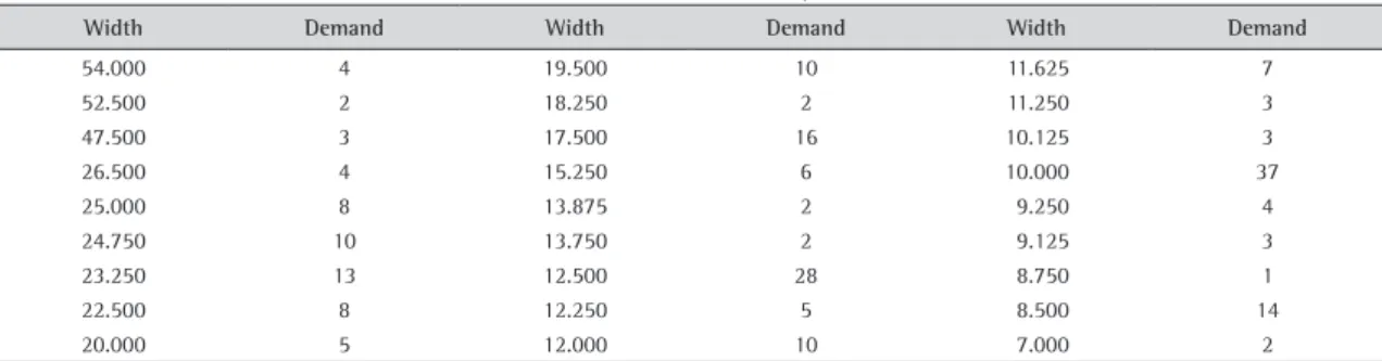
Table 2 presents the input parameters of the example considered by Haessler (1975), which has 27 required item types and master rolls of W = 141.

Table 3 presents the cutting plan obtained by MSHP. We set MAXR 11= to follow the restriction imposed by Haessler. Parameters a and β are as indicated before, as well the setup cost. The other parameters are as indicated previously in Table 1. We note that Haessler generated 8 cutting patterns with trim loss of 0.41% when using 25 master rolls. MSHP generates 7 cutting patterns with the same trim loss 0.41% using 25 master rolls. The descriptor I1 for this instance indicated that 24.89628 master rolls are needed to fulfill the required

demand. Thus, 25 master rolls are the optimum solution with respect to trim loss. We note that in Vahrenkamp (1996) a similar solution was obtained.

Parameter βG of Algorithm 2 is set to allow the generation of cutting patterns with low trim loss. In practice, we just provide a portion of the items to be scheduled using Model (14-20) by setting ui. Note that we maintain the upper bound indicated by Haessler in the calculation (r MINU_i/ ). Like parameter aG, βG is also varied in the first phase. The stop criteria over MINU is for the end of the process. After all, there may be scenarios in which it is not possible to achieve such usability of the master roll. A relation of main parameters and the corresponding values or ranges of Haessler’s SHP and MSHP is indicated in Table 1. We note parameter MAXTL is implicit in variable t of Model (14-20), while Haessler considered the interval [0.006W;0.03W] for it.

Table 1. Main parameters of Haessler (1975)’s SHP and MSHP.

SHP MINR MAXR Fraction a of MINU li ui

Haessler (1975) I2−1 Number of knives [0.5;0.9]

0 for all item types, except the one with

highest d_i

/

i r MINU

MSHP 1 Number of knives Fixed scalar by iteration 0 Algorithm 2

Table 2. Haessler’s example.

Width Demand Width Demand Width Demand

54.000 4 19.500 10 11.625 7

52.500 2 18.250 2 11.250 3

47.500 3 17.500 16 10.125 3

26.500 4 15.250 6 10.000 37

25.000 8 13.875 2 9.250 4

24.750 10 13.750 2 9.125 3

23.250 13 12.500 28 8.750 1

22.500 8 12.250 5 8.500 14

4.2. CutGen1 benchmark instances

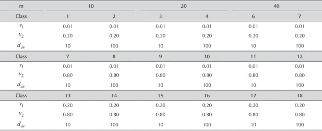
The generator CutGen1 for 1DCSP was developed by Gau & Wäscher (1995) and is available at https://web.fe.up.pt/~esicup/problem_generators/. We adopt the same 18 classes proposed by Foerster & Wäscher (2000), and considered by Yanasse & Limeira (2006) and Cui et al. (2015). Each class features 100 instances. A class is characterized by the number of item types (m), the size of the master roll (W), the values v₁ and v2 to

determine the width of the items in the range

[

v W v W1 , 2

]

and the average of the demands (dav). Table 4 presents the parameters to generate such classes.

Table 3. Cutting plan generated by MSHP to Haessler’s example.

Pattern Frequency Trim Loss

24.75(1), 23.25(1), 17.5(1), 12.5(2), 12(1), 10(3), 8.5(1) 10 0

54(1), 25(1), 22.5(1), 20(1), 19.5(1) 4 0

26.5(1), 25(1), 22.5(1), 19.5(1), 17.5(1), 12.25(1), 9.25(1), 8.5(1) 4 0

47.5(1), 23.25(1), 15.25(1), 12.5(1), 11.625(2), 10.125(1), 9.125(1) 3 0

52.5(1), 15.25(1), 12.5(2), 11.25(1), 10(3), 7(1) 2 0

20(1), 19.5(1), 15.25(1), 13.875(2), 13.75(2), 12.25(1), 10(1), 8.75(1) 1 0

19.5(1), 18.25(2), 17.5(2), 12.5(1), 11.625(1), 11.25(1) 1 14.625

Sum 25 14.625

Table 4. Parameters for the random instances of Cutgen1.

m 10 20 40

Class 1 2 3 4 6 7

1

v 0.01 0.01 0.01 0.01 0.01 0.01

2

v 0.20 0.20 0.20 0.20 0.20 0.20

av

d 10 100 10 100 10 100

Class 7 8 9 10 11 12

1

v 0.01 0.01 0.01 0.01 0.01 0.01

2

v 0.80 0.80 0.80 0.80 0.80 0.80

av

d 10 100 10 100 10 100

Class 13 14 15 16 17 18

1

v 0.20 0.20 0.20 0.20 0.20 0.20

2

v 0.80 0.80 0.80 0.80 0.80 0.80

av

d 10 100 10 100 10 100

These classes are divided into three groups: (G1) six classes of small items (v1=0.01 and v2=0.20); (G2) six

classes of miscellaneous items (v1=0.01 and v2=0.80); and (G3) six classes of large items (v1=0.20 and v2=0.80).

Classes with low demand have dav=10 and the ones with high demand have dav=100. The parameter m admits the following values: 10, 20, and 40 item types. For all classes, W=1000 and the same seed (‘1994’) of the original paper was used.

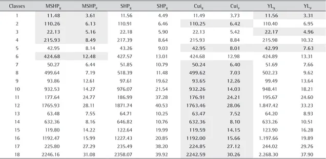
Table 5 presents the computational results from MSHP compared to Haessler (1975) (denoted as SHP), Cui et al. (2015) (denoted as Cui) and Yanasse & Limeira (2006) (denoted as YL). MSHP_R represents the average number of master rolls and MSHP_P the average pattern count. The other approaches follow the same subscript definitions. The concept of non-dominated solutions is used to compare the approaches, as in Cui et al. (2015). The results in bold indicate that the analyzed approach presents non-dominated (average) results for that class. MSHP is non-dominated by any of the other approaches in 5 of the 18 classes. Cui et al. (2015) contains 13 non-dominated classes, Yanasse & Limeira (2006) contains 3 non-dominated classes, while Haessler (1975) is dominated in all classes.

These results show our MSHP seems to perform better in scenarios of smaller-width items types (group G1) in relation to the object’s width, while Cui is better in scenarios of large-width item types (groups G2 and G3). Indeed, for instances like of G2 and G3, MSHP tends to generate patterns with minimum waste in the first iterations of its first phase and with significantly waste in the last iterations – SHP has a similar behavior. This feature may not be overcome in its second phase. On the other hand, the sequence value correction of Cui et al. (2015) efficiently addresses such quest for these scenarios. For the 1800 instances, the average computation time of MSHP is 3.60 seconds and of SHP is less than 0.1 seconds. In general, the computation time is not an issue for 1DCSP methods based on SHP algorithms. The computation time for the algorithm in Cui is 1.14 seconds on a computer Intel Core i7 CPU 2.20GHz RAM 8GB, and for the algorithm in YL is 7.83 seconds on a computer Intel Celeron CPU 266MHz RAM 128MB.

4.3. Fiber benchmark instances

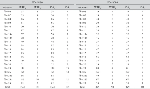
Umetani et al. (2003) provided 40 practical instances from a chemical fiber industry. These instances are available at Umetani (2018). Table 7 presents the computational results from MSHP by using two different setting parameters, following the approach of Cui et al. (2015). For example, the instance name “fiber29” means

29

m= , and parameter W is equal to 5180 or 9080. When possible, we consider equal size (width) items of the same type. In Tables 7 and 8, each row shows the difference of the instances in relation to the costs of the master roll and the setup. The average computation time of an instance was 3.36 seconds for MSHP.

Considering setup as an auxiliary objective (c_r=W c, _s=100), MSHP requires 2 more master rolls (=1551-1549) and 46 fewer patterns (=194-148) than Cui for instances with W=5180, and same quantity of master rolls (=876-876) and 17 fewer patterns (=124-105) than Cui for instances with W=9080. Considering equal objective costs (cr=cs=W _{), MSHP requires 8 additional master rolls (=1568-1560) and 36 fewer patterns (=159-123) than} Cui for instances with W=5180. For instances with W=9080, MSHP requires the same 879 master rolls and 18 fewer patterns (=116-98) than Cui. The average computation time of the algorithm Cui is 1.445 seconds. These results show that MSHP yields Cui in scenarios of larger objects (W=9080). In other words, also considering the results of previous section, MSHP seems to perform better than Cui when the relative width of the item types are smaller

Table 5. Computational results of CutGen1 instances per class.

Classes MSHPR MSHPP SHPR SHPR CuiR CuiP YLR YLP

1 11.48 3.61 11.56 4.49 11.49 3.73 11.56 3.31

2 110.26 6.13 110.91 6.46 110.25 6.42 110.40 6.95

3 22.13 5.16 22.18 5.90 22.13 5.42 22.17 4.96

4 215.93 8.49 217.39 8.64 215.93 8.84 215.98 10.32

5 42.95 8.14 43.26 9.03 42.95 8.01 42.99 7.63

6 424.68 12.48 427.57 13.01 424.68 12.98 424.89 13.31

7 50.27 6.44 51.85 10.79 50.24 6.40 51.69 7.66

8 499.64 7.19 518.39 11.48 499.62 7.03 502.23 9.62

9 93.86 12.61 97.61 19.62 93.65 12.26 99.49 13.64

10 932.53 14.27 976.07 21.54 932.26 14.03 948.41 18.21

11 177.64 24.77 186.99 37.28 176.91 24.21 195.67 24.60

12 1765.93 28.11 1871.74 40.53 1763.46 28.06 1.847.42 33.23

13 63.48 7.55 64.71 10.25 63.47 7.52 64.20 8.93

14 632.36 8.16 646.82 10.76 632.36 8.10 633.26 10.51

15 119.80 14.22 122.64 19.99 119.59 14.15 123.90 16.28

16 1192.47 15.99 1227.43 20.85 1192.00 15.66 1.197.66 19.89

17 225.80 27.29 235.49 38.20 224.85 27.12 244.02 29.76

18 2246.16 31.08 2358.07 39.92 2242.59 30.26 2.268.30 37.90

Table 6. Computational results of CutGen1 instances per class group.

MSHPR MSHPP SHPR SHPR CuiR CuiP YLR YLP

G1 137.91 7.34 138.81 7.92 137.91 7.57 138.00 7.75

G2 586.65 15.57 617.11 23.54 586.02 15.33 607.49 17.83

G3 746.68 17.38 775.86 23.33 745.81 17.14 755.22 20.55

Average 490.41 13.43 510.59 18.26 489.91 13.34 500.24 15.37

in relation to the object’s width. In relation to SHP, as the algorithm does not consider parameters cr and cs, we chose not report results for each instance. However, for instances with W=5180, SHP provided a total of 1559 master rolls and 212 setups, while for W = 9080 it provided a total of 880 master rolls and 116 setups, with average computation time less than 0.1 seconds. Assuming a scenario as Table 7 (cr=W and cs=100), which is more adequate to SHP, the MHSP yields SHP.

Table 7. Computational results of Fiber instances withcr=W and cs=100.

W = 5180 W = 9080

Instances MSHPR MSHPP CuiR CuiP Instances MSHPR MSHPP CuiR CuiP

fiber06 33 5 33 5 fiber06 19 4 19 3

fiber07 33 4 33 4 fiber07 19 3 19 4

fiber08 86 4 86 6 fiber08 48 3 48 4

fiber09 53 7 53 7 fiber09 29 4 29 5

fiber10 69 5 69 7 fiber10 39 4 39 5

fiber11 67 5 67 7 fiber11 38 4 38 6

fiber13a 56 7 56 7 fiber13a 32 5 32 5

fiber13b 28 4 28 5 fiber13b 16 3 16 4

fiber14 48 5 47 10 fiber14 27 4 27 5

fiber15 57 5 57 8 fiber15 32 4 32 5

fiber16 82 10 82 11 fiber16 47 6 47 6

fiber17 83 8 83 8 fiber17 47 5 47 6

fiber18 96 8 96 10 fiber18 54 6 54 7

fiber19 133 9 133 9 fiber19 73 10 73 11

fiber20 32 8 32 8 fiber20 19 5 19 6

fiber23 141 13 141 18 fiber23 80 7 80 9

fiber26 190 12 190 13 fiber26 107 7 107 9

fiber28a 84 9 83 27 fiber28a 48 6 48 7

fiber28b 118 12 118 13 fiber28b 67 8 67 8

fiber29 62 8 62 11 fiber29 35 7 35 7

Total 1.551 148 1.549 194 Total 876 105 876 122

Table 8. Computational results of Fiber instances withcr=W and cs=W.

W = 5180 W = 9080

Instances MSHPR MSHPP CuiR CuiP Instances MSHPR MSHPP CuiR CuiP

fiber06 33 5 34 4 fiber06 19 4 19 4

fiber07 33 4 34 3 fiber07 19 3 19 4

fiber08 86 4 86 6 fiber08 48 3 48 4

fiber09 54 5 55 5 fiber09 29 4 30 4

fiber10 70 4 70 6 fiber10 39 4 39 5

fiber11 67 6 67 7 fiber11 38 4 38 5

fiber13a 57 5 56 7 fiber13a 32 5 32 5

fiber13b 28 4 28 5 fiber13b 16 3 16 4

fiber14 49 4 48 6 fiber14 27 4 27 5

fiber15 58 4 57 7 fiber15 32 4 32 5

fiber16 84 7 83 8 fiber16 47 6 47 6

fiber17 85 5 83 8 fiber17 47 5 47 5

fiber18 96 8 96 11 fiber18 55 5 54 7

fiber19 134 7 133 9 fiber19 74 5 74 7

fiber20 32 8 32 8 fiber20 19 5 19 6

fiber23 144 8 142 13 fiber23 80 7 81 8

fiber26 191 9 191 12 fiber26 107 7 107 9

fiber28a 86 8 84 11 fiber28a 49 5 48 8

fiber28b 119 10 119 12 fiber28b 67 8 67 8

fiber29 62 8 62 11 fiber29 35 7 35 7

5. Conclusion

Due to its relevance, the 1DCSP-S is a classical problem in OR which has been tackled by several authors. MSHP is a sequential heuristic procedure based on the aspiration criteria presented by Haessler in the 1970s. The main feature of the algorithm is a cutting pattern generator model that generates patterns with the best compromise considering utilization and pattern repetition. The computational results indicate its quality for pattern reduction.

MSHP is a simple algorithm. Thus, its coding can be easily performed. We note that obtaining satisfactory results for a class of problems, or even for different classes, is different from obtaining satisfactory results for a single instance of each class, in relation to parameter setting. MSHP is able to provide excellent results and the setting parameter task involves only a few parameters. Our experimental tests show MSHP is able to obtain better results in scenarios of small item types in relation to the master roll (Group 1 of CutGen1) or larger master roll (fiber instances with W=9080) than other approaches of the literature. Furthermore, such parameters are easily adapted to the preferences of the decision-maker that may prioritize setup reduction, cutting waste reduction, a trade-off between both objectives, or even to allow overproduction.

For future research, MSHP may also adapt to the 1DCSP-S with multiple master roll lengths or include the open-stack minimization problem.

References

Araujo, S., Poldi, K., & Smith, J. (2014). A genetic algorithm for the one-dimensional cutting stock problem with setups. Pesquisa Operacional, 34(2), 165-187. http://dx.doi.org/10.1590/0101-7438.2014.034.02.0165.

Aliano Filho, A., Moretti, A. & Pato, M. (2017). A comparative study of exact methods for the bi-objective integer one-dimensional cutting stock problem. The Journal of the Operational Research Society, 69, 1-18. http://dx.doi.org/10.1057/s41274-017-0214-7. Belov, G., & Scheithauer, G. (2007). Setup and Open-Stacks Minimization in One-Dimensional Stock Cutting. INFORMS Journal on

Computing, 19(1), 27-35. http://dx.doi.org/10.1287/ijoc.1050.0132.

Cherri, A. C., Arenales, M. N., Yanasse, H. H., Poldi, K. C., & Gonçalves Vianna, A. C. (2014). The one-dimensional cutting stock problem with usable leftovers - A survey. European Journal of Operational Research, 236(2), 395-402. http://dx.doi.org/10.1016/j.ejor.2013.11.026. Cui, Y., Zhao, X., Yang, Y., & Yu, P. (2008). A heuristic for the one-dimensional cutting stock problem with pattern reduction.

Proceedings of the Institution of Mechanical Engineers. Part B, Journal of Engineering Manufacture, 222(6), 677-685. http://dx.doi. org/10.1243/09544054JEM966.

Cui, Y., Zhong, C., & Yao, Y. (2015). Pattern-set generation algorithm for the one-dimensional cutting stock problem with setup cost. European Journal of Operational Research, 243(2), 540-546. http://dx.doi.org/10.1016/j.ejor.2014.12.015.

Diegel, A., Miller, G., Montocchio, E., van Schalkwyk, S., & Diegel, O. (2006). Enforcing minimum run length in the cutting stock problem. European Journal of Operational Research, 171(2), 708-721. http://dx.doi.org/10.1016/j.ejor.2004.09.039.

Cemil Dikili, A., Sarıöz, E., & Akman Pek, N. (2007). A successive elimination method for one-dimensional stock cutting problems in ship production. Ocean Engineering, 34(13), 1841-1849. http://dx.doi.org/10.1016/j.oceaneng.2006.11.008.

Eilon, S. (1960). Optimizing the shearing of steel bars. Journal of Mechanical Engineering Science, 2(2), 129-142. http://dx.doi. org/10.1243/JMES_JOUR_1960_002_022_02.

Foerster, H., & Wäscher, G. (2000). Pattern reduction in one-dimensional cutting stock problems. International Journal of Production Research, 38(7), 1657-1676. http://dx.doi.org/10.1080/002075400188780.

Gau, T., & Wäscher, G. (1995). CUTGEN1: A problem generator for the standard one-dimensional cutting stock problem. European Journal of Operational Research, 84(3), 572-579. http://dx.doi.org/10.1016/0377-2217(95)00023-J.

Gilmore, P. C., & Gomory, R. E. (1961). A Linear Programming Approach to the Cutting-Stock Problem. Operations Research, 9(6), 849-859. http://dx.doi.org/10.1287/opre.9.6.849.

Gilmore, P. C., & Gomory, R. E. (1963). A Linear Programming Approach to the Cutting Stock Problem - Part II. Operations Research, 11(6), 863-888. http://dx.doi.org/10.1287/opre.11.6.863.

Haessler, R. W. (1975). Controlling Cutting Pattern Changes in One-Dimensional Trim Problems. Operations Research, 23(3), 483-493. http://dx.doi.org/10.1287/opre.23.3.483.

Henn, S., & Wäscher, G. (2013). Extensions of cutting problems: setups. Pesquisa Operacional, 33(2), 133-162. http://dx.doi.org/10.1590/ S0101-74382013000200001.

Kantorovich, L. (1960). Mathematical methods of organizing and planning production. Management Science, 6(4), 366-422. http:// dx.doi.org/10.1287/mnsc.6.4.366.

Kolen, A., & Spieksma, F. (2000). Solving a bi-criterion cutting stock problem with open-ended demand: a case study. The Journal of the Operational Research Society, 51(11), 1238-1247. http://dx.doi.org/10.1057/palgrave.jors.2601023.

Metzger, R. W. (1958). Stock slitting. In R. W. Metzger. Elementary mathematical programming. New York: Wiley.

Mobasher, A., & Ekici, A. (2013). Solution approaches for the cutting stock problem with setup cost. Computers & Operations Research, 40(1), 225-235. http://dx.doi.org/10.1016/j.cor.2012.06.007.

Umetani, S. (2018). Benchmark instances for the one-dimensional cutting stock problem. Osaka: Osaka University. Retrieved in 05 November 2017, from https://sites.google.com/site/shunjiumetani/benchmark.

Vahrenkamp, R. (1996). Random search in the one-dimensional cutting stock problem. European Journal of Operational Research, 95(1), 191-200. http://dx.doi.org/10.1016/0377-2217(95)00198-0.

Yanasse, H. (1997). On a pattern sequencing problem to minimize the maximum number of open stacks. European Journal of Operational Research, 100(3), 454-463. http://dx.doi.org/10.1016/S0377-2217(97)84107-0.