SYNCHRONOUS MACHINE FIELD CURRENT CALCULATION TAKING
INTO ACCOUNT THE MAGNETIC SATURATION
Ernesto Ruppert Filho
∗Francisco Liszt Nunes Jr.
∗Sidney Osses Nunes
∗∗ Systems and Energy Control Department - Computer and Electrical Engineering School – Campinas University,
DSCE-FEEC-UNICAMP, P.O. Box: 6101, CEP: 13081-970 Campinas-SP-Brasil
ABSTRACT
A synchronous machine dynamic mathematical model including the saturation effect is presented. The satura-tion modeling deals with the linkage flux mathematical model and uses the machine d-axis and q-axis magne-tizing curves. Results are shown in the form of V curves and comparisons with calculations using non-saturated and saturated reactances are done showing a consider-able difference in the excitation current values. Com-parisons with experimental data are done.
KEYWORDS: Synchronous machine, dynamic model, saturation model, magnetic saturation.
1
INTRODUCTION
Synchronous machines are intensively used as generators due to its very good voltage and frequency regulation characteristics. To study the control of the generated real and reactive power it is necessary to have a very accurate mathematical dynamic model to implement ef-ficient simulations.
A synchronous generator, connected to an infinite bus which voltage is the generator rated voltage, has its sta-ble operating point defined by the following rated
val-Artigo submetido em 18/12/00
1a. Revis˜ao em 16/05/01; 2a. Revis˜ao 21/02/02
Aceito sob recomenda¸c˜ao do Ed. Assoc. Prof. Denizar C. Martins
ues: armature voltage, apparent power, speed, power factor and excitation voltage. This set of values defines the load angle, armature winding current and excitation current.
In general, due to economic reason, the synchronous generator operates in the saturated part of the mag-netizing curve so that the variables are very sensitive to load and excitation current variations. So it is necessary to include magnetic saturation effects in the generator mathematical model to make it more accurate to rep-resent the machine both in transient and steady-state operation.
The magnetic saturation plays an important role in the definition of the excitation current required for the gen-erator operation when producing very well defined real and reactive power, that is, generator operating with a very well defined real power and power factor since it is fed by the rated bus voltage and driven by a mechanical torque corresponding to its real power (load).
The excitation current is very important to power sys-tem engineers for electrical energy syssys-tem generators stability calculation initialization. The most realistic value of the excitation current is also very important to the excitation system design.
simula-tion, include the saturation effects in the mathematical dynamic model.
Several methods to represent the magnetic saturation in synchronous machines have been presented in the liter-ature like [1, 2, 3, 4] dealing, in general, with modifi-cations in the d-axis and q-axis reactance. Generator manufacturers use to provide the machine d-axis and q-axis synchronous non-saturated and saturated reactance to the utility customers. These reactance are frequently used by the electrical energy system engineers to carry transient stability studies, system stability for small dis-turbances and other types of studies that depend funda-mentally from generator variable values at the instant of a disturbance occurrence.
In this paper it is presented a generator dynamic mathe-matical model where the differential equations are writ-ten in terms of the d-axis and q-axis stator and rotor winding linkage fluxes and currents as seen in [5], in-cluding a sub model of magnetic saturation in the iron (saturation in the air is not considered) involving the d-axis and q-axis generator magnetizing curves.
In spite of the model be a dynamic model, in this pa-per it is presented only steady-state simulation results through the generator V curves obtained using non-saturated reactance, non-saturated reactance and the model mentioned above. The results for an hydrogenerator, which data are in the appendix, are compared and com-mented.
2
SYNCHRONOUS MACHINE
MATHE-MATICAL DYNAMIC MODEL
A dynamic mathematical model of a synchronous ma-chine operating as a generator is shown below [5]:
vq=−rsiq+ωr ωbΨd+
p ωbΨq,
vd=−rsid−ωr ωbΨq+
p ωbΨd,
vo=−rsio+ p
ωbΨo, pθr=ωr,
0 =raqiaq+ p
ωbΨaq, pθe=ωe,
vf=rfif+ p
ωbΨf, δ=θr−θe,
0 =radiad+ p
ωbΨad, ωm=
2
pωr,
Te= 3 2
P
2 1
ωb(Ψdiq−Ψqid),
pωr= P
2J (Ta−Te),
(1)
where: vd andvq are the q-axis and d-axis components of the stator winding phase voltage,vf is the field wind-ing voltage,iq andid are the qd components of the sta-tor winding current,if, iaq andiadare respectively, the
field winding, q-axis and d-axis damping winding cur-rents, rs is the stator winding per phase electrical re-sistance, rf,raq and rad are the field winding electrical resistance, the q-axis and the d-axis damping winding electrical resistances respectively, ωr is the rotor elec-trical angular speed, ω b is the base electrical angular
speed (which is used to calculate reactance), Ψq and Ψd
are the stator winding q and d-axis phase linkage fluxes per second (voltages), Ψf, Ψaqand Ψadare respectively,
the field winding, the q-axis and the d-axis damping winding linkage fluxes per second (voltages), p is the differential operator, P is the machine pole number, J
is the inertia moment of the machine and turbine ro-tors, Ta is the driving torque (turbine torque),Teis the machine electromagnetic torque, θris the angular posi-tion of the q-axis referred to the stator winding phase-a magnetic field axis,θeis the angular position of the max-imum value of the stator winding phase-a voltage,ωeis the stator winding voltage electrical angular speed (syn-chronous speed),ωmis the mechanical angular speed and
δ is the load angle of the machine.
The variables with subscript o are the corresponding zero sequence variables that are important when non-balanced studies need to be made.
The linkage flux/sec variables (Ψ ) can be written as:
ψq=−Xℓsiq+ψmq, ψd=−Xℓsid+ψmd,
ψo=−Xℓsio, ψaq=Xℓaqiaq+ψmq,
ψf =Xℓf if +ψmd, ψad=Xℓadiad+ψmd,
(2)
where: Xls,Xlaq,Xlad,Xlf are the stator winding leak-age reactance, q-axis and d-axis damping winding and the field winding leakage reactance respectively.
Ψmqand Ψmd are the q-axis and d-axis magnetizing
fluxes per second which are also the q-axis and d-axis magnetizing fluxes/second (magnetizing voltages)
If magnetic saturation is not considered it can be writ-ten:
ψmq=Xmq imq,
ψmd=Xmdimd, (3)
q-axis and d-axis magnetizing currents.
imq=−iq+iaq,
imd=−id+if+iad. (4)
Using equations (2) and (4) it is possible to write:
ψq =−Xqiq+Xmqiaq, ψd=−Xdid+Xmdiad,
Xq =Xℓs+Xmq, Xd =Xℓs+Xmd,
(5)
Xq, Xd are non-saturated synchronous reactance. No-tice that all the rotor machine variables and parameters are referred to the stator winding.
3
SATURATION AFFECTING MACHINE
STEADY-STATE VARIABLES
Utilities use to use the non-saturated and the saturated values of the d-axis and q-axis synchronous reactance to perform electrical system dynamic studies and use to ask to synchronous machine manufacturers for the non-saturated and non-saturated values of the d-axis and q-axis synchronous reactance. That is the same as to provide the non-saturated and saturated values of the d-axis and q-axis magnetizing reactance because leakage reactance is considered constant and non-saturated.
The non-saturated values ofXmdandXmqare the slopes of the air-gap lines in the (Ψm,,imd) and (Ψmq,imq) mag-netizing curves, respectively, as shown in the figure 2.
The saturated value of Xd is the inverse of the short-circuit ratio. The saturated d-axis magnetizing reac-tance can be calculated asXmds=Xd−Xls.
The short-circuit ratio is the ratio between the no-load field current at rated voltage and frequency and the field current necessary to have the short-circuit rated current at rated frequency in the short-circuited machine arma-ture winding.
The saturated value ofXq is taken normally as 95% of the non-saturated value for large hydrogenerators and the saturated q-axis magnetizing reactance can be cal-culated asXmqs=Xq−Xls.
Using the dynamic mathematical model provided in [5], constituted by the equations (1) to (5), it can calculate the values of the several variables involving the machine using magnetizing reactance Xmd and also,Xd andXq
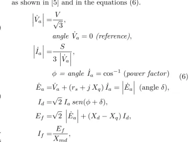
as shown in [5] and in the equations (6).
Va˙
=
V √
3,
angle Va˙ = 0(reference),
˙
Ia
=
S
3 Va˙
,
φ = angle Ia˙ = cos−1
(power factor) ˙
Ea= ˙Va+ (rs+j Xq) ˙Ia = Ea˙
(angleδ),
Id=√2Iasen(φ+δ),
Ef =√2
˙
Ea
+ (Xd−Xq)Id,
If = Ef
Xmd,
(6)
where: ˙Va and V are respectively the phase armature voltage phasor and the line to line armature voltage (rms), ˙Ia is the armature current phasor, S is the ap-parent power (VA),If is the field current andId is the peak d-axis armature current
Using these equations it is possible to plot the machine V curve which is the curve of
Ia˙
againstIf for a given
real power and variable power factor. These calculations were done for two different cases using the machine ex-ample data presented in the appendix.
In thecase 1the non-saturated magnetizing reactance
Xmd andXmq are used in the equations (6) and in the
case 2the saturated valuesXmds andXmqsare used in
the equations (6).
Figure 1 shows the V curves for the 2 cases above and for the machine rated real power (P = 1 pu). It is pos-sible to see that to get the same stator winding current (armature current) it is necessary to increase the field current about 15% when machine is saturated (in the sense of using saturated values of the reactance Xmds
andXmqsto represent the saturation effects). It can be seen also that the curves are almost parallel, mainly in the inductive load region.
Table 1 shows, for thecase 1, the values of the
steady-state field current (If) when the armature voltage is V = 1 pu for three different values of the apparent power S (S = 1.00 pu, S = 1.10 pu and S = 1.15 pu) and machine rated power factor.
Table 2 shows the same values for the case 2 where
the saturation effect is included by considering Xmds
andXmqs.
(sat-urated in the sense of using sat(sat-urated magnetizing reac-tance) is about 9% larger than the field current shown incase 1(non-saturated).
0 500 1000 1500 2000 2500 3000 1
1.1 1.2 1.3 1.4 1.5 1.6 1.7 1.8
x 104
IFIELD(Amps)
IARMATURE(Amps)
(1) (2)
Figure 1: V curves for cases 1 and 2 (real power = 1.0 pu).
Table 1: Field current the case 1.
S (pu) 1.00 1.10 1.15
If(A) 1886 1976 2021
Table 2: Field current for the case 2.
S (pu) 1.00 1.10 1.15
If(A) 2059 2149 2194
4
SATURATION MODEL USING D-AXIS
AND Q-AXIS MAGNETIZING CURVES
In this item a synchronous machine dynamic mathemat-ical model is developed to included the saturation using the equations (1) to (5) and also the machine d-axis and q-axis magnetizing curves.
As it can be seen in the equations (1) and (2) the terms
pΨq andpΨd transform themselves inpΨmq andpΨmq,
respectively when the saturation in the air is neglected. To calculate them it is necessary to have the d-axis and q-axis magnetizing curves in a mathematical form.
Those curves can be provided by the machine manufac-turer. The machine manufacturer can construct them in the machine design time or in its final tests according to the IEEE Standard [6]. A mathematical representation
through hyperbolic functions is used in this paper for the machine example.
The curves for the machine used in this paper (ap-pendix) are shown in figure 2 where Ψm and Im are
the magnetizing flux/s and magnetizing current respec-tively.
-4 -3 -2 -1 0 1 2 3 4
x 10
4
-2 -1.5 -1 -0.5 0 0.5 1 1.5 2
x 104
Im(Amps) Ψm(Volts)
d
q
Figure 2: d-axis and q-axis magnetization curves.
In this paper unbalanced studies are not considered, so substituting equations (2) in (1), eliminating the zero sequence equation, and using the hyperbolic representa-tion of (Ψmd,imd) and (Ψmq,imq) curves (appendix), it can be written:
pΨmq= dΨmq
dimq dimq
dt ,
pΨmd= dΨmd
dimd dimd
dt , p imq=−p iq+p iaq, p imd=−p id+p if+p iad,
fc= 1
Xℓs dΨmq
dimq ,
fd= 1
Xℓs dΨmd
dimd,
faq= 1
Xℓaq dΨmq
dimq ,
fq= 1
Xℓf dΨmd
dimd,
fad= 1
Xℓad dΨmd
dimd .
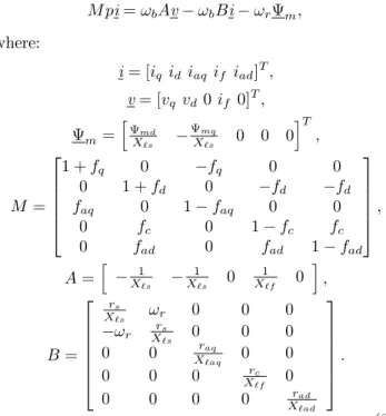
It is possible, after some simple algebraic calculations, to compact the six first equations (1) including the equa-tions (7) in one matrix equation as below:
M pi=ωbAv−ωbBi−ωrΨm,
where:
i= [iq id iaq if iad]T, v= [vq vd 0if 0]T,
Ψm=
Ψ
md
Xℓs −
Ψmq
Xℓs 0 0 0
T
,
M =
1 +fq 0 −fq 0 0
0 1 +fd 0 −fd −fd
faq 0 1−faq 0 0
0 fc 0 1−fc fc
0 fad 0 fad 1−fad
,
A= −X1ℓs −
1 Xℓs 0
1 Xℓf 0
,
B=
rs
Xℓs ωr 0 0 0
−ωr rs
Xℓs 0 0 0
0 0 raq
Xℓaq 0 0
0 0 0 rc
Xℓf 0
0 0 0 0 rad
Xℓad
.
(8)
The values of the factorsfq, fd, faq, ff, fadan the fluxes Ψmdand Ψmqare calculated at each step of the
differen-tial equations numerical integration using the d-axis and q-axis magnetization curves (Ψmd,,imd) and (Ψmq,imq) seen in the figure 2 and which algebraic equations are in the appendix.
5
SIMULATION
RESULTS
USING
THE PRESENTED MATHEMATICAL
MODEL
The mathematical model represented by the equations (1) to (5) is a linear dynamic model so that it is possible to derive a steady-state model from it simply making the derivative of the fluxes equal to zero and the algebraic complex equations (6) can be found [5].
Due to the non-linear character of the equations (7) and (8) the presented mathematical model can not be worked to find algebraic equations to represent the steady-state operation. The steady-state must be reached by solving the differential equations and wait-ing for the end of the transient state.
So to get the V curve using this model it is necessary to solve the differential equations (7) and (8), for each field current or field voltage, and wait for the steady-state to find the armature current.
Figure 3 shows the V curves for the 3 cases studied in this paper: curve 1 corresponds to the case 1 where the non-saturated reactance Xmd and Xmq were used with the linear model, curve 2 corresponds to the case 2 where the saturated reactanceXmds andXmqs were used with the linear model and curve 3 corresponds to the case 3 where the non-linear model presented in this paper that takes into account the machine magnetizing curves were used. The real power in this case is the rated power.
For each armature current value there are different val-ues of the generator excitation current. For the arma-ture rated current (12450 A, rated power factor) it
0 500 1000 1500 2000 2500 3000 3500 1
1.1 1.2 1.3 1.4 1.5 1.6 1.7
x 104 IARMATURE(Amps)
IFIELD(Amps) (1) (2) (3)
Figure 3: V curves for cases 1, 2 and 3 (real power = 1.0 pu).
has three different excitation currents, depending on the way the magnetic saturation is considered. For the way before named as 1 the excitation current is 1886 A, for the way named 2 it is 2059 A and for the third way it is 2184 A.
The same table shown before is shown now in table 3, for the new model. In this case a dynamic simulation was run to find the steady-state operating point.
Table 3: Field current for the new model.
S (pu) 1.00 1.10 1.15
If(A) 2184 2280 2329
6
EXPERIMENTAL RESULT AND
COM-PARISONS
Measurement carried out in the power plant where the generator is included, during the starting tests, had shown the excitation current of 2291 A for rated op-eration condition.
The errors can be calculated for the same operating con-ditions shown in the V curves of figure 3:
ε1=
2291−1886
2291
×100% = 17,76%
ε2=
2291
−2059
2291
×100% = 10,13%
ε3=
2291
−2184
2291
×100% = 4,23%
(9)
The experimental result shows that the presented non-linear model give a more accurate field current compared with the field current got from the linear model using non-saturated reactance or saturated reactance.
7
CONCLUSIONS
The linear model shown in the equations (1) to (5), with non-saturated or saturated reactance, despite to be fre-quently used by the engineers for steastate and dy-namic calculations, is not accurate. The errors in the stead-state field current are very high as it can be seen (items 5 and 6 (equations 8)).
The non-linear model presented in this paper, despite to spend more computational time to give the results, is more accurate to be used in electrical power system calculations.
ACKNOWLEDGMENT
Special thanks to Brazilian Research Council (CNPq) and S˜ao Paulo Research Foundation (FAPESP) for fund the authors Francisco Liszt Nunes Jr. and Sidney Osses Nunes.
REFERENCES
G. Shaskshaft, and P. Henser, “Model of generator satu-ration for use in power system studies”, IEE Proc., Vol. 126, No. 8, August 1979, pp. 759-763.
R.G. Harley, D.J.N. Limebeer, and E. Chirricizzi, “Comparative study of saturation methods in syn-chronous machine models”, IEE Proc., Vol. 127, Pt. B, No. 1, Jan 1980, pp. 1-7.
A.M. El-Serafi, and A.S. Abdallah, “Effect of saturation on steady-state stability of synchronous machines connected to an infinity bus system”, IEEE Trans. On Energy Conversion, Vol. 6, No. 3, Sept. 1991, pp. 514-521.
F.P. De Mello, and L.N. Hannett, “Representation of saturation in synchronous machines”, IEEE Trans. on Power Systems, Vol. PWRS-1, No. 4, Nov. 1986, pp. 8-18.
P.C. Krause, Analysis of Electric Machinery, McGraw Hill, 1986.
IEEE Std 115-1995, Guide: Test Procedures for Syn-chronous Machines, in IEEE Standards Collection Electric Machinery, Published by IEEE, 1997.
A
APPENDIX
In this appendix the data of the hydrogenerator used as example in the paper are presented. This machine is ready to start operation in the Brazilian Electrical System.
Rated values:
345 MVA – 16 kV – 60 Hz – 0.9 pf – 80 poles.
Parameters: J = 28.8x10⁶
Js2
, Xℓs= 0.1144 Ω, Xℓf= 0.0916 Ω,
Xℓad= 0.1175 Ω, Xℓaq= 0.0787 Ω, Xmd= 0.5747 Ω,
Xmq= 0.3524 Ω, rs(75oC) = 0.00181 Ω, rf= (75oC)
= 0.000247 Ω, rad(75oC) = 0.00247 Ω, raq(75oC) =
0.00533 Ω, Xmds= 0.5 Ω, Xmqs= 0.3312 Ω. (all the rotor parameters are referred to the stator side).
Magnetizing curves presented in the figure 2 were pro-vided by the manufacturer and can be represented by the following hyperbolic equations:
ψmd=cd[tanh(adi2mdSign(imd) +bdimd) +kdimd],
ψmq=cq[tanh(aqi2mqSign(imq) +bqimq) +kqimq],
where: