doi: 10.1590/0101-7438.2016.036.03.0447
A MODEL-BASED HEURISTIC FOR THE IRREGULAR STRIP PACKING PROBLEM
Luiz Henrique Cherri
1*, Maria Ant´onia Carravilla
2and Franklina Maria Bragion Toledo
1Received October 10, 2015 / Accepted September 13, 2016
ABSTRACT.The irregular strip packing problem is a common variant of cutting and packing problems. Only a few exact methods have been proposed to solve this problem in the literature. However, several heuristics have been proposed to solve it. Despite the number of proposed heuristics, only a few methods that combine exact and heuristic approaches to solve the problem can be found in the literature. In this paper, a matheuristic is proposed to solve the irregular strip packing problem. The method has three phases in which exact mixed integer programming models from the literature are used to solve the sub-problems. The results show that the matheuristic is less dependent on the instance size and finds equal or better solutions in 87,5% of the cases in shorter computational times compared with the results of other models in the literature. Furthermore, the matheuristic is faster than other heuristics from the literature.
Keywords: matheuristics, irregular strip packing, mixed integer programming models.
1 INTRODUCTION
Irregular cutting and packing problems have been extensively studied over the last five decades. The problem consists of cutting irregular pieces from a given object. Overlaps between pieces must be avoided, and the pieces must be entirely inside the object. The irregular strip packing problem is a common variant of this problem where the object is a rectangular board with fixed width and a length that is to be minimized. This problem is found in several industries, such as garment and shoe manufacturing, sheet metal cutting and furniture. From an economic point of view, the solution to the problem reduces the amount of material necessary to produce the pieces, decreasing the waste and hence the production costs.
The irregular strip packing problem is NP-complete (Fowler et al., 1981), and because of its difficulty only a few exact approaches have been proposed to solve it. Carravilla et al. (2003)
*Corresponding author.
1Universidade de S˜ao Paulo – USP, Avenida Trabalhador S˜ao-carlense, 400, 13566-590 S˜ao Carlos, SP, Brasil. E-mails: [email protected]; [email protected]
presented an approach based on implicit enumeration and constraint logic programming. The first mixed integer programming model was presented by Fischetti & Luzzi (2009). Alvarez-Valdes et al. (2013) improved this last model and proposed a branch and cut method to solve it. The authors also described a mixed integer programming model based on the compaction model presented by Gomes & Oliveira (2006). A new MIP model that represents the board by a mesh of dots (grid) was introduced by Toledo et al. (2013). In this model, the pieces can only be positioned at the dots of a grid, and consequently, the solution optimality is subject to the grid used. Recently, Le˜ao et al. (2016) proposed a model where the pieces can be placed continuously along the x-axis and at discrete positions along the y-axis to combine the best characteristics of the previous models.
In contrast to the number of exact approaches, many heuristics have been proposed to solve the problem. These methods can be classified as constructive heuristics or improvement heuristics (Bennell & Oliveira, 2009). Constructive heuristics aim to build a solution to the problem using some particular strategy. “Bottom-left-fill” heuristic (Burke et al., 2006), “2-exchange heuristic” (Gomes & Oliveira, 2002) and “TOPOS” (Oliveira et al., 2000) are examples of constructive heuristics. Given a feasible solution, improvement heuristics search for better-quality solutions. The fast neighborhood search developed by Egeblad et al. (2007) and the simulated annealing heuristic proposed by Oliveira & Ferreira (1993) are examples of improvement heuristics. A complete review of heuristics is presented in Bennell & Oliveira (2009).
Recently, rather complex and sophisticated heuristic methods have been developed. Umetani et al. (2009) presented an overlap minimization algorithm based on translations of pieces along ver-tical and horizontal directions. The algorithm is incorporated into a guided local search in order to solve the strip packing problem. Imamichi et al. (2009) proposed an iterated local search heuris-tic to solve the problem. The local search swaps the position of a pair of pieces in the solution, and a non-linear programming separation algorithm ensures non-overlap between the pieces. An extended local search heuristic to solve the problem was proposed by Leung et al. (2012). Two neighborhoods are used to change piece positions during the local search. The feasibility of the solution is reached by non-linear programming separation and compaction models. To solve the problem, Sato et al. (2012) proposed two constructive heuristics using the concept of collision-free regions and identifying pieces that fit well. These heuristics are combined with a simulated annealing algorithm in order to obtain better solutions. A compaction model is used to reduce the length of the solutions obtained in each iteration of the algorithm. Elkeran (2013) proposed a heuristic where in the first step the pieces are clustered in pairs and then a guided cuckoo search heuristic is used to pack the pieces into the board. This heuristic achieves the best results in the literature for the irregular strip packing problem.
to the problem. Following the constructive phase, the improvement phase is applied. This phase also uses the dotted board model that is now combined with a Variable Neighborhood heuristic to find better-quality solutions. Finally, in the compaction phase, a model based on the compaction model presented in Gomes & Oliveira (2006) with additional constraints is solved in order to compact the solution found in the improvement phase removing some gaps resulting from the grid dependence of the dotted board model.
The contributions of this paper are the following: (1) a method that constructs a solution for instances with several items using an iterative procedure based on a mixed integer programming model; (2) new constraints are proposed for the Toledo et al. (2013) model in order to perform local searches with different grids. (3) Using a model based on Gomes & Oliveira (2006), a new compaction model is proposed, and (4) a model where the pieces are continuously placed on the board is integrated with models that consider pieces placed on discrete points.
This paper is organized as follows: section 2 provides a problem definition and describes the dotted board model that is used in the solution method. The model-based heuristic is presented in section 3. Section 4 contains the computational experiments performed on instances from the literature. Finally, section 5 provides conclusions and presents some highlights.
2 PROBLEM DEFINITION
The irregular strip packing problem consists of cutting irregular pieces from a rectangular board of fixed width (W) and infinite length. The objective is to minimize the board length (L) used.
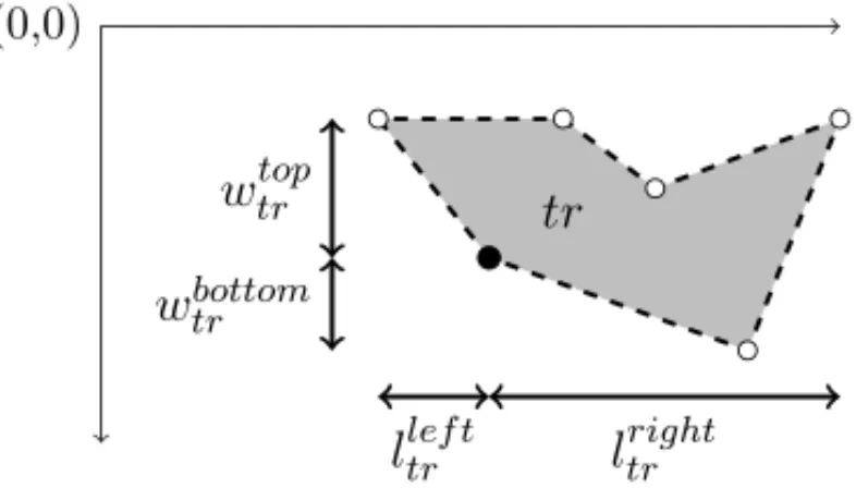
Each piece is represented by a set of points corresponding to its vertices. One of these vertices is chosen to be its reference point, which is used to allocate the piece on the board. Given a piece of typet at rotationr, considerltrle f t (ltrright), the horizontal distance from the leftmost (rightmost) piece vertex to the reference point, andwbot t omtr (wt optr ), the vertical distance from the bottom
(top) piece vertex to the reference point. These distances are important for defining the feasible region in the board where the piece can be allocated. Figure 1 illustrates these constants.
(0,0)
l
lef ttr
l
right tr
w
bottomtr
w
toptr
tr
Figure 1–Defining the constantsltrle f t,wtrbot t om,lrighttr andwtrt op.
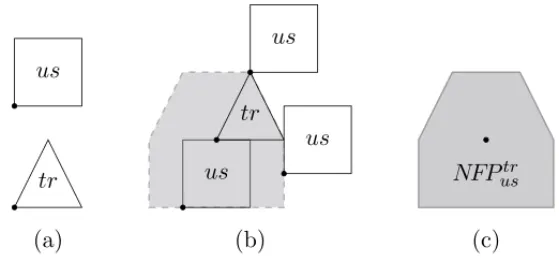
theNFP is illustrated in Figure 2. Considering the piecest at rotationr anduat rotationsas in Figure 2a, theNFPustr is the polygon drawn by the reference point ofuwhileuorbits around t, always touching but not overlappingt, as illustrated in Figure 2b. The complete NFPustr is presented in Figure 2c. With this structure, verifying if the piecestat rotationranduat rotation soverlap is now reduced to analyzing the relative position between the reference point of piece uand the polygonNFPustr.
us
tr
tr
us
us
us
NFP
ustr(a)
(b)
(c)
Figure 2–The nofit polygon structure. (a) presents the pieces used to build theNFP, which is built in (b). In (c), theNFPis displayed.
The second condition is that the pieces must be entirely inside the board. This condition is en-sured with the inner-fit polygon (IFP) structure of a piece with respect to the board. The inner-fit polygon of a piecet at rotationr (IFPtr) represents all the positions where the reference point
of piecet at rotationr can be placed keeping the piece entirely inside the board, as shown in Figure 3. In the figure, the gray area defines theIFPtr. Note that as we have an upper bound for
the board lengthL, theIFPlimits the placement of the pieces. More details on these geometric structures can be found in Bennell & Oliveira (2008).
tr
tr
tr
IFP
tr0 L
Figure 3–The inner-fit polygon structure.
In order to make this text self-contained, the dotted board model proposed in Toledo et al. (2013) is presented next. For this model, the piece reference points can only be positioned on dots from a given setDthat represents the board. The refinement of this grid is defined by the constantsgx
To define the positioning of the pieces on the board, considerT a set of piece types, i.e., types of pieces with different shapes. Consider alsoRt, the set of rotations of piecet. The binary variable
δtrd is 1 if the reference point of a piece of typet ∈T at rotationr ∈Rt is on dotd ∈Dand 0
otherwise. It is important to highlight that the gridDis defined using the distancesgx andgy.
The number of variablesδdtr depends on these constants. The feasible placement positions for each piece typetat rotationrare the dotsd ∈DinsideIFPtr, which define theDIFPtr set.
For each pair of piece typest at rotationr andu at rotations, the points that overlap when piece t is placed at dotd ∈ DIFPtr are represented by dots inside NFPustrIFPus, that is,
d ∈DNFPd,tr us .
The Dotted Board Model (DBM) is the following:
min.: L (1)
s.t.:(dx+ltrright)×δdtr ≤L, d ∈DIFPtr,t ∈T,r ∈Rt, (2)
δusd′ +δdtr ≤1, d′∈DNFPd,tr
us ,d∈DIFPtr,t,u∈T,r ∈Rt,s∈Ru, (3)
d∈DIFPtr,r∈Rt
δdtr =qt, t ∈T,r ∈Rt, (4)
δtrd ∈ {0,1}, d ∈DIFPtr,t ∈T,r ∈Rt, (5)
L ≥0. (6)
wheredxis the x-coordinate of dotd.
The objective function (1) together with constraints (2) minimizes the board length. Constraints (3) guarantee that the pieces do not overlap. Constraints (4) ensure that the demandqt for each
piece typet is met. The domain of the variables is defined by constraints (5) and (6). Further details on the dotted board model can be found in Toledo et al. (2013).
The Dotted Board Model, (1)-(6), is independent on the type of grid that is used. In the following, instead of using regular grids as in Toledo et al. (2013), the grid of dots based on the piece dimensions proposed by Cherri et al. (2016) is used, aiming to reduce the number of board dots.
For each piece of typet ∈ T at rotationr ∈ Rt, a gridDtr is created based on the constants
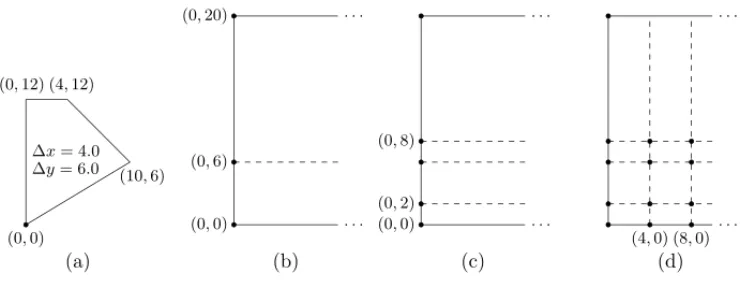
gtrx andgtry that define the distance between the dots along the horizontal and vertical axes re-spectively. The value ofgxtr is given by the minimum horizontal distance between each pair of vertices of piece of typet at rotationr, but limited by the minimum grid resolutiongmin. The
constantgtry is obtained by the same procedure, but by using the minimum vertical distance be-tween each pair of vertices of piece of typetat rotationr. The minimum grid resolution impacts directly the solution quality. The grid for each piece typet at rotationr is generated using the constantsgxtr andgtry.
touch the boundaries of the board. Along the horizontal axis, the vertical lines are equally spaced bygxtr units, starting from the leftmost point of the board (Fig. 4(d)). TheDtr set comprises the
intersection points between the horizontal and vertical lines.
(0,0)
(10,6)
(4,12)
(0,12)
∆x= 4.0
∆y= 6.0
. . . . . .
(0,0)
(0,6)
(0,20)
. . . . . .
(0,0)
(0,2)
(0,8)
. . . . . .
(4,0) (8,0)
(a) (b) (c) (d)
Figure 4–Building the mesh by piece for the piece in (a)
3 3-PHASE MATHEURISTIC (3PM)
The 3-Phase Matheuristic is based on two mathematical models, the Dotted Board Model of (Toledo et al., 2013) and the compaction model of Gomes & Oliveira (2006). Our objective is to obtain good-quality solutions in a short computational time. The proposed method has three phases:
• Constructive Phase: finding an initial feasible solution using the Dotted Board Model;
• Improvement Phase: improving the initial solution using the Dotted Board Model;
• Compaction Phase: improving the best solution found so far using the linear compaction model.
In the subsections (3.1)-(3.3), the three phases of 3PM are described in detail.
3.1 3PM – Constructive Phase
The objective of the constructive phase is to build an initial feasible solution for the problem. The grid used is a grid by piece with a minimum resolutiongmin, large enough to ensure a good
trade-off between the computational time and solution quality. The value ofgminwas defined
using preliminary computational experiments.
This phase is based on the relax-and-fix strategy. Consider the decision variablesδtrd, which are 1 (one) if a piece of typetat rotationris assigned to dotdand 0 (zero) otherwise. These variables are split into four sets:
) set of variables associated with pieces that are positioned on the board, but can still perform some movements;
) set of variables associated with pieces that can be freely positioned on the board;
) set of variables associated with waiting pieces, that are not considered in the resolution step.
Initially, setsŴ,andare empty, setincludes all the pieces, and the parametersµandµ′, the limits in the x-axis for the setsŴand, are set to zero.
In each step of the constructive phase a small number of pieces belonging to the setis assigned to, the setsŴandare redefined based on the parametersµ′andµ, i.e. the pieces with the reference point positioned in the interval[0, µ′)define setŴ, the pieces with the reference point positioned in the interval[µ′, µ]define set, and the sub-problem defined by the setsŴ,and is solved. In the final step, setis empty and a feasible solution to the complete problem is obtained by solving the associated sub-problem.
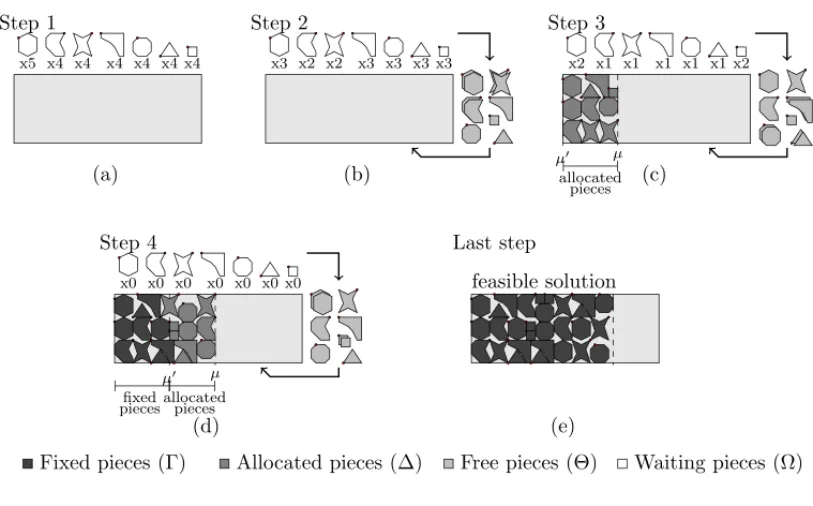
Figure 5 illustrates the steps of the constructive phase based on an example with seven piece types and a total of 29 pieces. The pieces associated with setsŴandare represented in black and dark gray, respectively. The pieces in setare represented in white above the board and the number of repetitions is written below each piece. The pieces in light gray, at the right-hand side of the board, represent set. In Figure 5(a) setsŴ,andare empty. In Figure 5(b), some pieces from the setare selected to form set. Figure 5(c) represents the solution for the problem in Figure 5(b), the setand the new set.
Figure 5(d) shows the solution of sub-problem in 5(c) where the pieces with reference point in the interval[0, µ)are fixed and new pieces are positioned on the board. The solution of the complete problem is presented in Figure 5(e).
In each step, a subset of elements from setis selected for set. The size of these subsets is σ, a number small enough to provide a fast solution and big enough for the pieces to fit well. Furthermore, the size is calculated so as to reduce the difference between the sizes of the subsets, and details are provided in Section 4.1. To form each set, the pieces are included one by one in the subset. The piece type selected is the one with the largest rate:
number of pieces of typetin the set number of pieces of typetin the instance(qt)
, ∀t ∈T.
This criterion was used in order to homogeneously distribute the different piece types in the solution.
To define each sub-problem model, consider subsetsM⊂DandW ⊂Dcontaining the board dots in the intervals[0, µ′)and[µ′, µ], respectively. The previous step solution is defined by δtrd,d ∈ D,t ∈ T,r ∈ Rt. Note thatŴ = {(d,t,r), δtrd = 1,d ∈ M,t ∈ T,r ∈ Rt}and
= {(d,t,r), δtrd = 1,d ∈ W,t ∈ T,r ∈ Rt}. The partial demand is represented byqt,
Step 1
x5 x4 x4 x4 x4 x4 x4
(a)
Step 2
x3 x2 x2 x3 x3 x3 x3
(b)
Step 3
x2 x1 x1 x1 x1 x1 x2
µ
µ′
allocated
pieces (c)
Step 4
x0 x0 x0 x0 x0 x0 x0
µ′ µ
fixed piecesallocatedpieces
(d)
Last step
feasible solution
(e)
Fixed pieces (Γ) Allocated pieces (Δ) Free pieces (Θ) Waiting pieces (Ω)
Figure 5–Steps of the Constructive Phase.
pieces of typetwith the reference point in subsetW. The constructive phase model (3PM–CPM) is given by (7)-(10):
min.: L (7)
s. t.:(2), (3), (5), (6),
d∈IFPtr,r∈Rt
δdtr =qt, t ∈T, (8)
¯
δdtr=1,d∈W
(1−δdtr)+
¯
δdtr=0,d∈W
δtrd ≤αt, t ∈T,r∈Rt, (9)
δdtr =1, (d,t,r)∈Ŵ. (10)
In the model (7)-(10), constraints (8) ensure that the partial demand will be met. Constraints (9) restrict the movements over the variables of setW. Specifically, one move is counted when a piece previously allocated in set W is moved outside setW or when a piece from setis allocated into setW. Two moves are counted when a piece previously allocated in set W is moved into setW. The upper bound for the moves isαt. Constraints (10) fix to the board the
Algorithm 1Constructive phase Input:SetsD,T and;
Output:A feasible solutionδ= {(d,t,r)|δdtr =1}; Initialize:
Calculateσ (number of pieces to form); Doδ=0,µ′=µ=0;
Constructive phase: While (= ∅)
Define the subsetsMandW; Do=∅;
Remove min{σ,||}pieces from the setand insert them into the set; Solve the sub-problem (CPM) obtaining the solutionδwith valueL; Doµ′=µandµ=L;
Returnδas the solution.
3.2 3PM – Improvement Phase
The Improvement Phase starts with the solution of the Constructive Phase and it is also performed in steps. In the first step,gminis equal to that used in the constructive phase, and after each step,
gmin is divided by two. Note that, as stated in Section 2, gmin is only a lower bound of the
grid resolution value. At the end of each step, the dots that contain reference points of pieces allocated are included into the grid of the next step. This ensures that the best solution found so far is feasible for the next step and leads to a good initial solution for the search. The search ends whengminis smaller than a thresholdmr. In each step, a variable neighborhood descent heuristic
(VND) is applied to improve the quality of the best solution found so far.
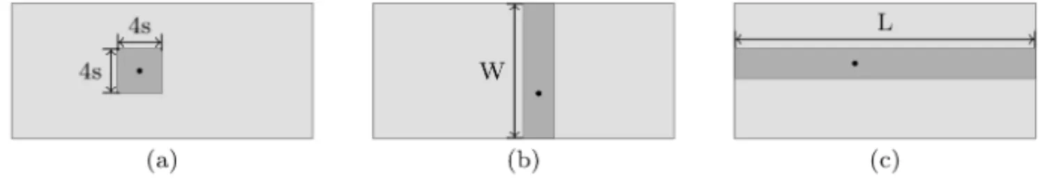
The VND heuristic is defined by applying successive local search procedures overKdifferent neighborhoods. The choice of a neighborhood is performed in a deterministic way. A final so-lution is a local optimum with respect to allKneighborhoods. The neighborhoods are defined allowing the pieces to move in the dots that are inside a small board region around the solution of the previous step,δ = {(d,t,r)|δdtr =1}. The shape of these regions defines the neighborhood that will be explored during the search. The first neighborhood is a small square with its center in the dot where the piece was positioned. The second neighborhood is a rectangle with the same height as the width of the board. The width of the rectangle is chosen so that the number of dots in the region is limited bymd. Finally, the third neighborhood is a rectangle with the length of the board. The height of the rectangle is also chosen so that the number of dots in the region is limited bymd. Figure 6 illustrates these three neighborhoods, where the dot represents the piece reference point and the highlighted rectangle the region where this reference point can move.
Figure 6–Representation of the neighborhoods for a piece reference point.
neighborhood is created to allow the pieces to move vertically. Finally, the third neighborhood aims to change the piece’s position over the layout length.
The sequence of the neighborhoods starts by the first neighborhood to restrict the feasible piece placement and then solve the problem. If the solution is not better than the best solution found so far, then the second neighborhood structure is applied. If the search over the second neigh-borhood structure does not improve the solution quality, then the third neighneigh-borhood structure is applied. If the third neighborhood does not improve the solution quality, then the step is termi-nated. During the process, if any of the three neighborhoods yields a solution better than the best solution found so far, then the search process restarts with the first neighborhood.
Each neighborhood can be represented by a model. Consider dtr as the set of dots belonging to
one neighborhood of dotd where the reference point of piecet at rotationrwas allocated in the previous iteration. The improvement phase model (3PM-IPM) is given as follows.
min.:L (11)
s.t.: (2), (3), (4), (5), (6),
δtd′′r′ =0, (d′,t′,r′)∈ {D\ dtr},t ∈T,r ∈Rt,d∈D. (12)
Constraints (12) limit the search domain to move each piece within the chosen neighborhood. Given a feasible solutionδ, the best solution of the model (11)-(12) is its best neighbor.
When there are no more neighborhoods to explore in VND, the grid is refined. With more dots to represent the board, there is a new range of feasible placement positions for each piece. The VND heuristic is performed again to improve the solution further. Algorithm 2 summarizes the improvement phase.
3.3 3PM – Compaction Phase
As the solution obtained in the Improvement Phase has the piece reference points positioned on specific dots, gaps may appear between pieces. Taking this into account, a compaction of this solution is essential to move the pieces as close as possible to each other. To compact a solution, we use the mixed integer linear model based on Gomes & Oliveira (2006) with some additional constraints. In this model, the positioning of each piece reference point is represented by a pair of continuous variables(xi,yi). To avoid overlaps between piecesi and j, the authors consider
Algorithm 2Improvement phase
Input:SetT; initial resolutiongmin; thresholdmr; a solutionδand its valueL;
Output:Improved solutionδ;
Initialize:
Choose the first neighborhood,N eigh =1; Improvement phase:
While (gmin>mr)
DefineDusinggmin;
Add the dots ofδtoD; While (N eigh≤3)
Findδ′the best neighbor solution ofδusing the neighbourhoodN eigh;
If (L′≥L), DoN eigh =N eigh+1; else, DoN eigh=1;δ=δ′;L=L′; Dogmin=gmin/2;
Return solutionδ;
to ensure that the pieces are on different sides of at least one of the linese∈Ei j. More details on
this model can be found in Gomes & Oliveira (2006) and Alvarez-Valdes et al. (2013). In order to define the additional constraints to be added to the Gomes & Oliveira (2006) model, consider the pieces individually, i.e., each piece is mapped according to its type and rotation by an unique integer. The total number of pieces is given byN =t∈T,r∈R
t dtr. All the pieces can be found
on the interval[1,N]. In addition, considerxi (yi),i =1, . . . ,N, the position on the x-axis
(y-axis) for eachδdt =1,∀d ∈ D. The new constraints imposed in Gomes & Oliveira (2006) model ensure that the pieces can move only over a small region of the board. These regions are defined as squares around the points where each piece is positioned. The sideλiof each square
is given based on the size of the bounding box of each pieceiand the number of pieces allocated and is defined in Section 4.1.
The Compaction Phase Model (3PM-CPM) is given as (13)-(19):
min.:L (13)
s.t.:lile f t ≤xi ≤L−lrighti , i =1, . . . ,N, (14)
wit op≤ yi ≤W −wibot t om, i =1, . . . ,N, (15)
αi j e(xj−xi)+βi j e(yj −yi)
≤γi j e+Big M(1−vi j e), 1≤i< j≤N,∀e∈ Ei j, (16)
e∈Ei j
vi j e ≥1, 1≤i < j ≤N, (17)
xi−λi ≤xi ≤xi+λi, i =1, . . . ,N, (18)
yi−λi ≤ yi ≤ yi+λi, i =1, . . . ,N, (19)
xi,yi ≥0, i =1, . . . ,N, (21)
L ≥0. (22)
whereαi j e,βi j eandγi j eare the coefficients of the lineeassociated with an edge ofNFPi j and
Big Mis large enough to make the constraint (16) a dummy constraint ifvi j e=0.
Constraints (14) associated with (13) define the objective function. Constraints (14) and (15) ensure that the piece is entirely inside the board, and constraints (16) and (17) guarantee that the pieces do not overlap. Constraints (18) and (19) allow the piece to move only within a given square. Finally, the variable domains are given by (20), (21) and (22).
The compaction phase is an iterative process, i.e., if an improved solution is found at the end of the compaction, the compaction is run again, starting from this improved solution. Algorithm 3 presents an outline of the compaction phase.
Algorithm 3Compaction phase Input:A feasible solutionδ;
Output: Compacted solution(x,y)andL; Initialize:
Obtainx,yandLfromδ; Defineλi;
Compaction phase: Do
Solve theC P M model obtaining the solutionx′,y′and lengthL′; If (L′<L)
Dox=x′,y=y′,L =L′andL′=0 Until (L′≥L)
Return(x,y)andLas the solution.
4 COMPUTATIONAL RESULTS
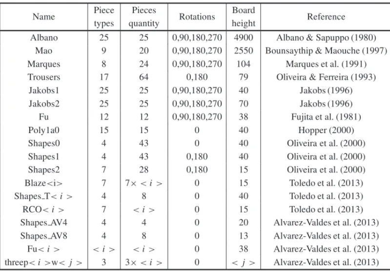
The computational experiments were performed on an Intel(R) Xeon(R) E5-2620 2.00GHz pro-cessor with 64 GB of memory running an Ubuntu 12.04 operating system. The methods were implemented in the C/C++ programming language, and the mathematical models were solved using IBM ILOG CPLEX 12.5. To perform the tests, instances from the literature, presented in Table 1, were used. The first column presents the instance name. Columns two and three present the number of piece types and the TOTAL number of pieces, respectively. The available rotations for the pieces and the height of the board are, respectively, presented in columns four and five. Finally, column six presents the reference in the literature of the instance.
Table 1–Instances used in the benchmark.
Name Piece Pieces Rotations Board Reference
types quantity height
Albano 25 25 0,90,180,270 4900 Albano & Sapuppo (1980)
Mao 9 20 0,90,180,270 2550 Bounsaythip & Maouche (1997)
Marques 8 24 0,90,180,270 104 Marques et al. (1991)
Trousers 17 64 0,180 79 Oliveira & Ferreira (1993)
Jakobs1 25 25 0,90,180,270 40 Jakobs (1996)
Jakobs2 25 25 0,90,180,270 70 Jakobs (1996)
Fu 12 12 0,90,180,270 38 Fujita et al. (1981)
Poly1a0 15 15 0 40 Hopper (2000)
Shapes0 4 43 0 40 Oliveira et al. (2000)
Shapes1 4 43 0,180 40 Oliveira et al. (2000)
Shapes2 7 28 0,180 15 Oliveira et al. (2000)
Blaze<i> 7 7×<i> 0 15 Toledo et al. (2013)
Shapes T<i> 4 8 0 40 Toledo et al. (2013)
RCO<i> 7 <i> 0 15 Toledo et al. (2013)
Shapes AV4 4 4 0 20 Alvarez-Valdes et al. (2013)
Shapes AV8 4 8 0 13 Alvarez-Valdes et al. (2013)
Fu<i> <i> <i> 0 38 Alvarez-Valdes et al. (2013) threep<i>w< j> 3 3×<i> 0 < j> Alvarez-Valdes et al. (2013)
in Subsection 4.2. The proposed matheuristic performance is compared with exact models and heuristic methods in Subsections 4.3 and 4.4, respectively.
4.1 Defining parameters and sets
In this section, the parameters used in the matheuristic are defined. These parameters were chosen based on preliminary computational experiments and on the features of each instance.
The initial value ofgminis two in order to generate a grid with a limited number of dots. The idea
is to lead the constructive phase to quickly obtain a solution. This parameter can generate some gaps among the pieces, but these gaps should be reduced in the improvement phase.
In each step of the constructive phase,σ elements ofmust be selected to form. The idea is to defineσ such that the subsetsof each iteration have a similar number of elements. After preliminary tests, we verified that problems with five pieces (in absolute number) or less are solved very fast using the model while problems with more than 12 pieces are difficult to solve within a time span adequate for a constructive phase. The value of sigma is defined as stated in Algorithm 4, whereamodbis the remainder of the division ofabyb.
In Algorithm 4, if the instance has less than five pieces, only one set with all the pieces is created. Otherwise, the subset size is given by the largest integer numberσ ∈ [5,min(12,t ∈T qt−1)]
Algorithm 4Defining sigma Input:Set, demandqt,t ∈T;
Output: σ;
If (|| ≤5) Return(||); Else
Doσ =5;sq=t∈Tqt;
Dos=min{12,sq}; While (s≥6) do
If (sqmods=0) Doσ =s; Return (σ);
Else if (sqmods≥sqmodσ) Doσ =s;
Dos =s−1; Return (σ);
the remainder is the largest possible, ensuring that the number of pieces in the final step will be the largest possible.
After the constructive phase, the improvement phase runs whilegmin≥mr, wheremr =0.5 to
make the pieces closer to each other. The number of dots in each neighborhood of the improve-ment phase must not be larger than the parametermd. In the initial tests,md = 3000, which results in the improvement model performing a fast local search.
Several preliminary tests were run to determine the value ofλifor each piece of typei, whereλi is a parameter of the compaction phase model (CPM). Depending on the position of the pieces and on the size of the region where these pieces can move, a pair of pieces could even change their relative positions.
These values are based on i) the number of pieces in the instance and ii) the size of the piece bounding box.
• For instances with less than 13 pieces the square around the reference point of piecei has a side equal toλi =max(lle f ti +lrighti , wbot t omi +wit om);
• For instances with 13 to 20 pieces the square around the reference point of piecei has a side equal toλi =max(lile f t+liright, wbot t omi +wt opi )/2;
4.2 Analysing the phases of 3PM
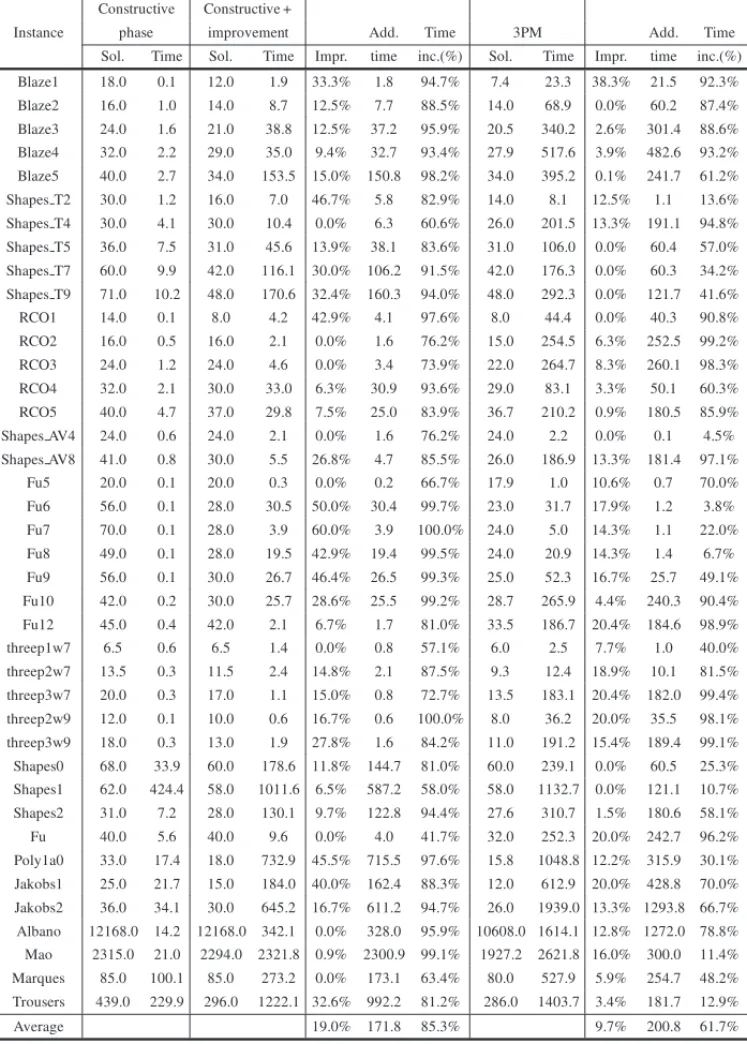
To demonstrate the importance of each phase of the 3PM, in Table 2, we summarize the results of each phase. The instance name is in the first column. In columns two and three, the constructive phase solution and time are shown. Columns four and five show the improvement phase solu-tion and its time, respectively. The improvement rate, the time increase and the percentage by which the computational time increases from the constructive phase to the improvement phase are depicted in columns six, seven and eight. In columns nine and ten, the solution value and its computational time are presented. Columns eleven, twelve and thirteen describe the improve-ment rate, the additional time and the percentage that the computational time increases compared with the constructive plus improvement phases.
As expected, the constructive phase obtained a solution with poor quality but in a short computa-tional time. Applying the improvement phase to the constructive phase solution on average leads to 19% improvement in the solution quality. The computational time increases by 171.8 seconds on average, varying from 0.1 to 2301 seconds depending on the instance.
On average, the solutions found by the complete matheuristic are 9.7% better when compared to the solutions found by the improved constructive phase. Furthermore, the computational time increases by 200 seconds on average, varying from 0.1 to 1294 seconds depending on the in-stance. Specifically, the compaction phase leads on average to 9.7% improvement in the solution quality; however, the computational time doubles.
Based on the results, it can be concluded that the compaction phase obtains better solutions. However, if a fast solution that has good quality is needed and less computational time is avail-able, the construction phase followed by the improvement phase should be used. If a more accurate solution is desired and using more computational time is not a problem, the complete solution method should be applied to the problem.
A variation of this matheuristic composed of only the construction and compaction phases was studied. The quality of the solutions obtained by thus variation was always worse than that of the complete matheuristic.
4.3 Performance of the matheuristic compared with mixed integer models
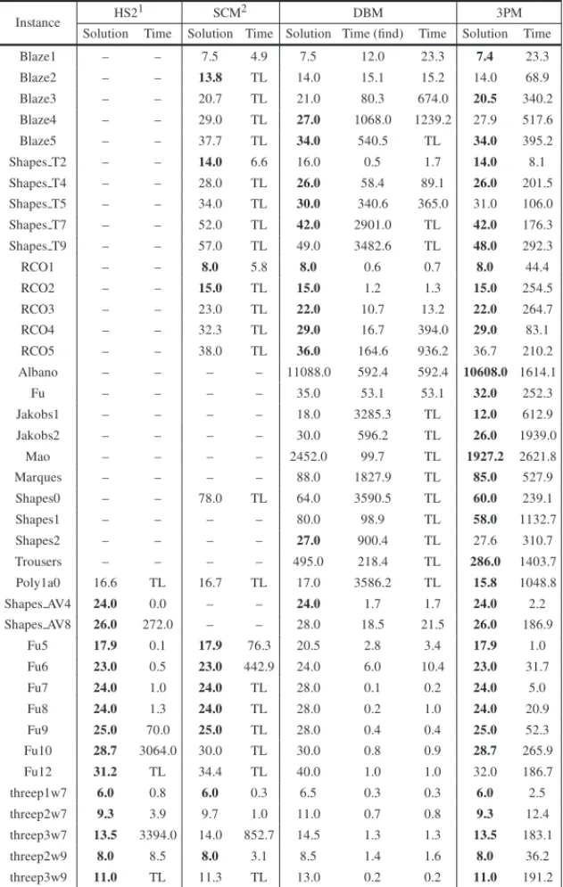
In this section, we analyzed the quality of the matheuristic solutions compared with the ex-act branch and cut method applied tothree models from the literature. Table 3 presents the results for solving instances using the HS2 model from Alvarez-Valdes et al. (2013), the semi-continuous model (SCM) from Le˜ao et al. (2016), the dotted board model (DBM) from Toledo et al. (2013) with the grid by pieces and by the proposed matheuristic. The results of HS2 and SCM were taken from Alvarez-Valdes et al. (2013) and Le˜ao et al. (2016), respectively. The specifications of their processor are better than the one used to solve the DBM and the proposed matheuristic3. Consequently, a comparison of the results is not unfair from the computational perspective. Moreover, each exact method was run for one hour.
Table 2–Evolution of solution values and time for the different phases of the 3PM.
Constructive Constructive +
Instance phase improvement Add. Time 3PM Add. Time
Sol. Time Sol. Time Impr. time inc.(%) Sol. Time Impr. time inc.(%) Blaze1 18.0 0.1 12.0 1.9 33.3% 1.8 94.7% 7.4 23.3 38.3% 21.5 92.3% Blaze2 16.0 1.0 14.0 8.7 12.5% 7.7 88.5% 14.0 68.9 0.0% 60.2 87.4% Blaze3 24.0 1.6 21.0 38.8 12.5% 37.2 95.9% 20.5 340.2 2.6% 301.4 88.6% Blaze4 32.0 2.2 29.0 35.0 9.4% 32.7 93.4% 27.9 517.6 3.9% 482.6 93.2% Blaze5 40.0 2.7 34.0 153.5 15.0% 150.8 98.2% 34.0 395.2 0.1% 241.7 61.2% Shapes T2 30.0 1.2 16.0 7.0 46.7% 5.8 82.9% 14.0 8.1 12.5% 1.1 13.6% Shapes T4 30.0 4.1 30.0 10.4 0.0% 6.3 60.6% 26.0 201.5 13.3% 191.1 94.8% Shapes T5 36.0 7.5 31.0 45.6 13.9% 38.1 83.6% 31.0 106.0 0.0% 60.4 57.0% Shapes T7 60.0 9.9 42.0 116.1 30.0% 106.2 91.5% 42.0 176.3 0.0% 60.3 34.2% Shapes T9 71.0 10.2 48.0 170.6 32.4% 160.3 94.0% 48.0 292.3 0.0% 121.7 41.6% RCO1 14.0 0.1 8.0 4.2 42.9% 4.1 97.6% 8.0 44.4 0.0% 40.3 90.8% RCO2 16.0 0.5 16.0 2.1 0.0% 1.6 76.2% 15.0 254.5 6.3% 252.5 99.2% RCO3 24.0 1.2 24.0 4.6 0.0% 3.4 73.9% 22.0 264.7 8.3% 260.1 98.3% RCO4 32.0 2.1 30.0 33.0 6.3% 30.9 93.6% 29.0 83.1 3.3% 50.1 60.3% RCO5 40.0 4.7 37.0 29.8 7.5% 25.0 83.9% 36.7 210.2 0.9% 180.5 85.9% Shapes AV4 24.0 0.6 24.0 2.1 0.0% 1.6 76.2% 24.0 2.2 0.0% 0.1 4.5% Shapes AV8 41.0 0.8 30.0 5.5 26.8% 4.7 85.5% 26.0 186.9 13.3% 181.4 97.1% Fu5 20.0 0.1 20.0 0.3 0.0% 0.2 66.7% 17.9 1.0 10.6% 0.7 70.0% Fu6 56.0 0.1 28.0 30.5 50.0% 30.4 99.7% 23.0 31.7 17.9% 1.2 3.8% Fu7 70.0 0.1 28.0 3.9 60.0% 3.9 100.0% 24.0 5.0 14.3% 1.1 22.0% Fu8 49.0 0.1 28.0 19.5 42.9% 19.4 99.5% 24.0 20.9 14.3% 1.4 6.7% Fu9 56.0 0.1 30.0 26.7 46.4% 26.5 99.3% 25.0 52.3 16.7% 25.7 49.1% Fu10 42.0 0.2 30.0 25.7 28.6% 25.5 99.2% 28.7 265.9 4.4% 240.3 90.4% Fu12 45.0 0.4 42.0 2.1 6.7% 1.7 81.0% 33.5 186.7 20.4% 184.6 98.9% threep1w7 6.5 0.6 6.5 1.4 0.0% 0.8 57.1% 6.0 2.5 7.7% 1.0 40.0% threep2w7 13.5 0.3 11.5 2.4 14.8% 2.1 87.5% 9.3 12.4 18.9% 10.1 81.5% threep3w7 20.0 0.3 17.0 1.1 15.0% 0.8 72.7% 13.5 183.1 20.4% 182.0 99.4% threep2w9 12.0 0.1 10.0 0.6 16.7% 0.6 100.0% 8.0 36.2 20.0% 35.5 98.1% threep3w9 18.0 0.3 13.0 1.9 27.8% 1.6 84.2% 11.0 191.2 15.4% 189.4 99.1% Shapes0 68.0 33.9 60.0 178.6 11.8% 144.7 81.0% 60.0 239.1 0.0% 60.5 25.3% Shapes1 62.0 424.4 58.0 1011.6 6.5% 587.2 58.0% 58.0 1132.7 0.0% 121.1 10.7% Shapes2 31.0 7.2 28.0 130.1 9.7% 122.8 94.4% 27.6 310.7 1.5% 180.6 58.1% Fu 40.0 5.6 40.0 9.6 0.0% 4.0 41.7% 32.0 252.3 20.0% 242.7 96.2% Poly1a0 33.0 17.4 18.0 732.9 45.5% 715.5 97.6% 15.8 1048.8 12.2% 315.9 30.1% Jakobs1 25.0 21.7 15.0 184.0 40.0% 162.4 88.3% 12.0 612.9 20.0% 428.8 70.0% Jakobs2 36.0 34.1 30.0 645.2 16.7% 611.2 94.7% 26.0 1939.0 13.3% 1293.8 66.7% Albano 12168.0 14.2 12168.0 342.1 0.0% 328.0 95.9% 10608.0 1614.1 12.8% 1272.0 78.8% Mao 2315.0 21.0 2294.0 2321.8 0.9% 2300.9 99.1% 1927.2 2621.8 16.0% 300.0 11.4% Marques 85.0 100.1 85.0 273.2 0.0% 173.1 63.4% 80.0 527.9 5.9% 254.7 48.2% Trousers 439.0 229.9 296.0 1222.1 32.6% 992.2 81.2% 286.0 1403.7 3.4% 181.7 12.9%
In Table 3, the first column presents the instance names. The second and third (fourth and fifth) columns present, respectively, the solution and time to prove the solution optimality of the Alvarez-Valdes et al. (2013) model (Le˜ao et al. (2016) model). Similarly, columns six and eight show the solution and time to prove the optimality of the dotted board model. Column seven depicts the time that this model took to find the best solution of the search. Finally, in columns seven and eight, the solution obtained by the proposed matheuristic method and its computational time are shown.
The proposed matheuristic obtained better or equal solutions in34out of 40 instances when compared with the best solutions of the other three methods. In the table, the best solution values are highlighted. Compared only with the dotted board model, the proposed matheuristic yielded better results for 27 out of 40 instances. For the majority of the instances, the compaction phase makes a difference by removing some gaps from the grid dependence of the dotted board model, resulting in better-quality solutions.
The computational time of the matheuristic is less than that of theHS2 model and SCM model only in the larger instances. In fact, this occurs because for small instances, the exact method can quickly find and prove the optimality of a solution while the matheuristic method needs to accomplish all three phases. Comparing the computational time of the dotted board model and the matheuristic, it can be observed that the exact method spends less time on small instances. The reason for this is the same as that for theHS2 and SCM model. It is important to highlight that in several cases, the matheuristic obtained better solutions than the dotted board model as the model depends on the grid used. Its improvement in terms of the solution quality is more distinguishable for the large instances.
The advantage of the 3-Phase Matheuristic is that in comparison with the exact approaches, the time to achieve the objective is less biased by the instance size.
As the constructive and improvement phases are based on the dotted board model, instances with many different piece types and/or huge boards such as Albano, Mao and Jakobs2 can lead to longer solution times in these phases of the solution method. Moreover, in the compaction phase, the model used does not take advantage of pieces of the same type, making instances as Trousers, Shapes1 and Shapes0 more difficult to solve in this phase.
On the other hand, the additional constraints included in the models of each phase attempt to overcome the problem, reducing the computational times. Additionally, the interactions between the approaches aim to benefit the solution quality.
4.4 Performance of the matheuristic compared with those of other heuristics
Table 3–Comparison of the results of the exact methods with the 3-Phase Matheuristic (3PM).
Instance HS2
1 SCM2 DBM 3PM
Solution Time Solution Time Solution Time (find) Time Solution Time
Blaze1 – – 7.5 4.9 7.5 12.0 23.3 7.4 23.3
Blaze2 – – 13.8 TL 14.0 15.1 15.2 14.0 68.9
Blaze3 – – 20.7 TL 21.0 80.3 674.0 20.5 340.2
Blaze4 – – 29.0 TL 27.0 1068.0 1239.2 27.9 517.6
Blaze5 – – 37.7 TL 34.0 540.5 TL 34.0 395.2
Shapes T2 – – 14.0 6.6 16.0 0.5 1.7 14.0 8.1
Shapes T4 – – 28.0 TL 26.0 58.4 89.1 26.0 201.5
Shapes T5 – – 34.0 TL 30.0 340.6 365.0 31.0 106.0
Shapes T7 – – 52.0 TL 42.0 2901.0 TL 42.0 176.3
Shapes T9 – – 57.0 TL 49.0 3482.6 TL 48.0 292.3
RCO1 – – 8.0 5.8 8.0 0.6 0.7 8.0 44.4
RCO2 – – 15.0 TL 15.0 1.2 1.3 15.0 254.5
RCO3 – – 23.0 TL 22.0 10.7 13.2 22.0 264.7
RCO4 – – 32.3 TL 29.0 16.7 394.0 29.0 83.1
RCO5 – – 38.0 TL 36.0 164.6 936.2 36.7 210.2
Albano – – – – 11088.0 592.4 592.4 10608.0 1614.1
Fu – – – – 35.0 53.1 53.1 32.0 252.3
Jakobs1 – – – – 18.0 3285.3 TL 12.0 612.9
Jakobs2 – – – – 30.0 596.2 TL 26.0 1939.0
Mao – – – – 2452.0 99.7 TL 1927.2 2621.8
Marques – – – – 88.0 1827.9 TL 85.0 527.9
Shapes0 – – 78.0 TL 64.0 3590.5 TL 60.0 239.1
Shapes1 – – – – 80.0 98.9 TL 58.0 1132.7
Shapes2 – – – – 27.0 900.4 TL 27.6 310.7
Trousers – – – – 495.0 218.4 TL 286.0 1403.7
Poly1a0 16.6 TL 16.7 TL 17.0 3586.2 TL 15.8 1048.8
Shapes AV4 24.0 0.0 – – 24.0 1.7 1.7 24.0 2.2
Shapes AV8 26.0 272.0 – – 28.0 18.5 21.5 26.0 186.9
Fu5 17.9 0.1 17.9 76.3 20.5 2.8 3.4 17.9 1.0
Fu6 23.0 0.5 23.0 442.9 24.0 6.0 10.4 23.0 31.7
Fu7 24.0 1.0 24.0 TL 28.0 0.1 0.2 24.0 5.0
Fu8 24.0 1.3 24.0 TL 28.0 0.2 1.0 24.0 20.9
Fu9 25.0 70.0 25.0 TL 28.0 0.4 0.4 25.0 52.3
Fu10 28.7 3064.0 30.0 TL 30.0 0.8 0.9 28.7 265.9
Fu12 31.2 TL 34.4 TL 40.0 1.0 1.0 32.0 186.7
threep1w7 6.0 0.8 6.0 0.3 6.5 0.3 0.3 6.0 2.5
threep2w7 9.3 3.9 9.7 1.0 11.0 0.7 0.8 9.3 12.4
threep3w7 13.5 3394.0 14.0 852.7 14.5 1.3 1.3 13.5 183.1
threep2w9 8.0 8.5 8.0 3.1 8.5 1.4 1.6 8.0 36.2
threep3w9 11.0 TL 11.3 TL 13.0 0.2 0.2 11.0 191.2
TL: Time limit.
– instances not addressed by Alvarez-Valdes et al. (2013).
The heuristics from the literature were run within different frameworks. The authors presented the best solution and the average solution found by their methods in several runs for each in-stance.
Table 4 presents the results obtained by 3PM and the results obtained by the two most recent heuristics from the literature. In the table, the first column displays the instance name. Columns two and three respectively present the solution found by 3PM and the computational time to obtain this solution. Columns four and five (six and seven) present analogous information for Leung et al. (2012) (Sato et al. (2012)) heuristic.
Table 4–Comparison of the results of the exact methods with the 3-Phase Matheuristic (3PM).
Instance 3PM Leung et al. (2012) Elkeran (2013) Solution Time Solution Time Solution Time Shapes0 60.0 239.1 59.7 10×1207.0 59.32 10×600.0 Shapes1 58.0 1132.7 53.7 10×1212.0 54.07 10×600.0 Shapes2 27.6 310.7 26.2 10×1205.0 26.21 10×600.0 Fu 32.0 252.3 31.7 10×600.0 31.46 10×600.0 Jakobs1 12.0 612.9 11.1 10×603.0 11.02 10×600.0 Jakobs2 26.0 1939.0 23.8 10×602.0 23.79 10×600.0 Albano 10608.0 1614.1 9969.5 10×1203.0 9959.24 10×600.0 Mao 1927.2 2621.8 1785.1 10×1204.0 1796.86 10×600.0 Marques 80.0 527.9 78.3 10×1204.0 77.37 10×600.0 Trousers 286.0 1403.7 246.7 10×1237.0 244.67 10×600.0
As 3PM is a deterministic procedure, it is run just once for each instance. In contrast, the heuris-tics proposed in Leung et al. (2012) and Elkeran (2013) are non-deterministic procedures that usually are run many times to ensure the quality of solution. The authors ran their heuristics 10 times that in the best case used 600 seconds for each time. Therefore, the proposed matheuristic is substantially faster and yields solutions in average six times faster than these heuristics.
On average, the solutions found by the matheuristic are 6.3% worse than the results obtained by Elkeran (2013) and Leung et al. (2012), which are the most recent heuristics in the literature.
5 CONCLUSIONS
A new matheuristic to solve the irregular strip packing problem combining mixed integer pro-gramming models from the literature is presented. The matheuristic is composed of three phases that use a model to solve each sub-problem. Combining different models, the proposed method takes advantage of the speed of the integer placement model and the solution quality of the linear placement model.
Comparing 3PM with heuristics form the literature, 3PM found solutions in smaller computa-tional times. Also, the quality of these solutions generally are near to the quality of the best solutions found in the literature.
APPENDIX A
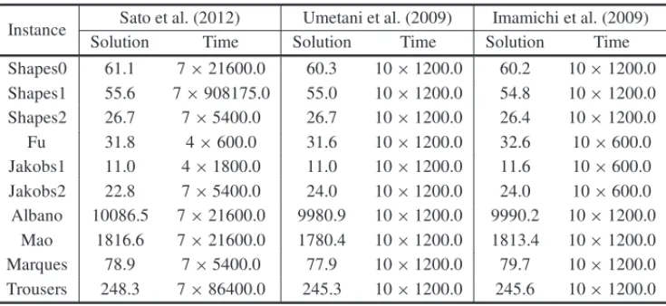
The results obtained for the heuristics presented in Umetani et al. (2009), Imamichi et al. (2009) and Sato et al. (2012) are shown in Table 5. This table has the same type of content of Table 4.
Table 5–Comparison of the results of the exact methods with the 3-Phase Matheuristic (3PM).
Instance Sato et al. (2012) Umetani et al. (2009) Imamichi et al. (2009)
Solution Time Solution Time Solution Time
Shapes0 61.1 7×21600.0 60.3 10×1200.0 60.2 10×1200.0
Shapes1 55.6 7×908175.0 55.0 10×1200.0 54.8 10×1200.0
Shapes2 26.7 7×5400.0 26.7 10×1200.0 26.4 10×1200.0
Fu 31.8 4×600.0 31.6 10×1200.0 32.6 10×600.0
Jakobs1 11.0 4×1800.0 11.0 10×1200.0 11.6 10×600.0
Jakobs2 22.8 7×5400.0 24.0 10×1200.0 24.0 10×600.0
Albano 10086.5 7×21600.0 9980.9 10×1200.0 9990.2 10×1200.0 Mao 1816.6 7×21600.0 1780.4 10×1200.0 1813.4 10×1200.0
Marques 78.9 7×5400.0 77.9 10×1200.0 79.7 10×1200.0
Trousers 248.3 7×86400.0 245.3 10×1200.0 245.6 10×1200.0
REFERENCES
[1] ALBANO A & SAPUPPOG. 1980. Optimal allocation of two-dimensional irregular shapes us-ing heuristic search methods.IEEE Transactions on Systems, Man, and Cybernetics,SMC-10(5): 242–248.
[2] ALVAREZ-VALDESR, MARTINEZA & TAMARITJ. 2013. A branch & bound algorithm for cutting and packing irregularly shaped pieces.International Journal of Production Economics,145(2): 463– 477.
[3] BENNELLJA & OLIVEIRAJF. 2008. The geometry of nesting problems: A tutorial.European Jour-nal of OperatioJour-nal Research,184(2): 397–415.
[4] BENNELLJA & OLIVEIRAJF. 2009. A tutorial in irregular shape packing problems.Journal of the Operational Research Society,60: S93–S105.
[5] BOUNSAYTHIPC & MAOUCHES. 1997. Irregular shape nesting and placing with evolutionary ap-proach. InSystems, Man, and Cybernetics, volume 4, pages 3425–3430.
[6] BURKEE, HELLIERR, KENDALLG & WHITWELLG. 2006. A new bottom-left-fill heuristic algo-rithm for the two-dimensional irregular packing problem.Operations Research,54(3): 587–601.
[8] CHERRI LH, CHERRIAC, CARRAVILLAMA, OLIVEIRAJF, TOLEDOFMB & VIANNAACG. 2016. An innovative data structure to handle the geometry of nesting problems. Technical report, Instituto de Ciˆencias Matem´aticas e de Computac¸˜ao, Universidade de S˜ao Paulo.
[9] EGEBLAD J, NIELSENBK & ODGAARDA. 2007. Fast neighborhood search for two- and three-dimensional nesting problems.European Journal of Operational Research,183(3): 1249–1266.
[10] ELKERAN A. 2013. A new approach for sheet nesting problem using guided cuckoo search and pairwise clustering.European Journal of Operational Research,231(3): 757–769.
[11] FISCHETTIM & LUZZII. 2009. Mixed-integer programming models for nesting problems.Journal of Heuristics,15(3): 201–226.
[12] FOWLERRJ, PATERSONM & TANIMOTOSL. 1981. Optimal packing and covering in the plane are np-complete.Inf. Process. Lett.,12(3): 133–137.
[13] FUJITAK, AKAGJIS & KIROKAWAN. 1981. Hybrid approach for optimal nesting using a genetic algorithm and a local minimization algorithm.Advances in Design Automation; American Society of Mechanical Engineers,65: 477–484.
[14] GOMESA & OLIVEIRAJF. 2006. Solving irregular strip packing problems by hybridising simulated annealing and linear programming.European Journal of Operational Research,171(3): 811–829.
[15] GOMESAM & OLIVEIRAJF. 2002. A 2-exchange heuristic for nesting problems.European Journal of Operational Research,141(2): 359–370.
[16] HOPPER E. 2000. Two-dimensional packing utilising evolutionary algorithms and other meta-heuristic methods. PhD thesis, University of Wales, Cardiff.
[17] IMAMICHIT, YAGIURAM & NAGAMOCHIH. 2009. An iterated local search algorithm based on nonlinear programming for the irregular strip packing problem.Discrete Optimization,6(4): 345– 361.
[18] JAKOBSS. 1996. On genetic algorithms for the packing of polygons.European Journal of Opera-tional Research,88(1): 165–181.
[19] LEUNG SC, LINY & ZHANGD. 2012. Extended local search algorithm based on nonlinear pro-gramming for two-dimensional irregular strip packing problem.Computers & Operations Research, 39(3): 678–686.
[20] LEAO˜ AAS, TOLEDOFMB, OLIVEIRA JF & CARRAVILLAMA. 2016. A semicontinuous MIP model for the irregular strip packing problem.International Journal of Production Research,54(3): 712–721.
[21] MANIEZZOV, STUTZLE¨ T & VOSSS. 2009. Matheuristics: Hybridizing Metaheuristics and Mathe-matical Programming. Annals of Information Systems. Springer.
[22] MARQUESVMM, BISPOCFG & SENTIEIRO JJS. 1991. A system for the compaction of two-dimensional irregular shapes based on simulated annealing. In: International Conference on Industrial Electronics, Control and Instrumentation, pages 1911–1916.
[23] OLIVEIRAJF & FERREIRAJ. 1993. Algorithms for nesting problems, applied simulated annealing. In Vidal RVV. (Ed., Lecture Notes in Economics and Maths Systems),396: 255–274.
[25] SATOAK, MARTINSTC & TSUZUKIMSG. 2012. An algorithm for the strip packing problem using collision free region and exact fitting placement.Computer-Aided Design,44(8): 766–777.
[26] TOLEDOFMB, CARRAVILLAMA, RIBEIROC, OLIVEIRAJF & GOMESAM. 2013. The dotted-board model: a new MIP model for nesting irregular shapes.International Journal of Production Economics,145(2): 478–487.
[27] UMETANIS, YAGIURAM, IMAHORIS, IMAMICHIT, NONOBEK & IBARAKIT. 2009. Solving the irregular strip packing problem via guided local search for overlap minimization.International