doi: 10.1590/0101-7438.2016.036.03.0533
A NON-ARCHIMEDEAN DEA MODEL TO ASSESS GROUP COMPARISONS
Geraldo da Silva e Souza and Eliane Gonc¸alves Gomes*
Received March 10, 2016 / Accepted October 20, 2016
ABSTRACT.We consider the use of the non-Archimedean infinitesimal epsilon in DEA-CCR models. The application of interest is defined by the performance measure of the Brazilian Agricultural Research Corporation research centers. We characterize an assurance region for the non-Archimedean element and suggest a value for it. Types of DMUs are compared using fractional regression models and quasi maximum likelihood inference. We conclude that the research centers aimed at studying specific agricultural products are dominant. The classic DEA-CCR performance measures and the solution provided by non-Archimedean model have Spearman correlation over 90%.
Keywords: non-Archimedean DEA models, non-zero weights, fractional regression.
1 INTRODUCTION
Since 1996, the Brazilian Agricultural Research Corporation (Embrapa) monitors the production of its research centers with the use of an evaluation system based on a single performance out-put and three inout-puts. The inout-puts of the process are capital, operational expenses and labor. The performance indicator (output) is a weighted average of 28 production attributes, classified into four production categories: (a) technical-scientific production; (b) production of technical pub-lications; (c) transfer of technologies and promotion of image; (d) development of technologies, products and processes. An efficiency measure is computed using Data Envelopment Analysis (DEA). See Souza et al. (1999) and Avila et al. (2014) for more details on Embrapa’s perfor-mance system. The system of weights used to combine individual output perforperfor-mance indicators into a single variable is complex. It uses the Law of the Categorical Judgments of Thurstone (Torgerson, 1958; Souza, 2002) and it is dependent on a normalization system that makes the individual performance indicators scale free.
In the context of the company’s new strategic guidelines for RD&I management and the propo-sition of a revised performance evaluation system, recently Souza & Gomes (2015a) suggested
*Corresponding author.
Embrapa, Secretaria de Gest˜ao e Desenvolvimento Institucional – SGI, PqEB Av. W3 Norte final, 70770-901 Bras´ılia, DF, Brasil.
the use of a three dimensional output, rearranging the attributes in three categories: (a) technical scientific production; (b) production of technical publications; (c) other activities. The system of weights used in these groupings is objective and based on Factor Analysis. In this context, the weighting system is data oriented and does not involve management pre-judgments regarding variable’s importance. This is a major technical improvement compared to the previous approach. All the performance classification is based on the ranks of the performance variables, measured on a per capita basis, as explained in Section 2. It is important to emphasize that pure ratios are not used here as production variables, although the use of ratios in DEA seems to be a valid approach according to the recent literature (Olsen et al., 2015). The approach we propose moti-vates the use of a DEA-CCR model with three inputs and three outputs. We point out that this new approach has much appeal basically for two reasons. Firstly, the company no longer uses the older method of performance evaluation, which is described in detail in Souza et al. (1999) and in Avila et al. (2014). Secondly, a weighting system common to all units is easier to understand at the management level and eliminates operational biases. Our objective here is to present an alternative approach robust to the determination of weights and, at the same time, useful to ob-tain a potential measure of goal achievement, as described in Souza & Gomes (2015a), allowing a convenient way to monitor production policies. In this context it is critical to have non-zero weights for all production variables in the DEA solution. A full discussion of the full perfor-mance evaluation system and of the DEA score used by Embrapa through the period 1996-2009 is presented in Avila et al. (2014).
The statistical inference in models where a DEA response is a dependent variable as a function of a set of covariates presents technical difficulties in two contexts. Firstly, the DEA calculations induce correlations among the DMUs. Of a more complex nature is the potential association of contextual variables with the error term. Simar & Wilson (2007, 2011), Badin et al. (2012), Souza & Gomes (2015b) discuss these problems in detail. Ramalho et al. (2010) suggest the use of the Papke & Wooldridge (1996) approach for two stage regressions. This approach is of our concern here, since the contextual variables are DMU types, unrelated to the performance score and therefore non endogenous. Gomes et al. (2008) give indication that the correlation induced by the design is not statistically significant for analysis of variance inferences when DEA re-sponses are subjected only to treatment effects, validating, in this context, the fractional regres-sions of Ramalho et al. (2010).
Our discussion proceeds as follows. In Section 2 we describe the performance model being con-sidered by Embrapa. In Section 3 we present the approach used to derive an assurance region and a value for the non-Archimedean constantε. Section 4 describes the fractional regression models we used to assess type differences in performance. Section 5 is on statistical results. Finally, in Section 6 we summarize our findings and present our conclusions.
2 EMBRAPA’S PERFORMANCE MODEL
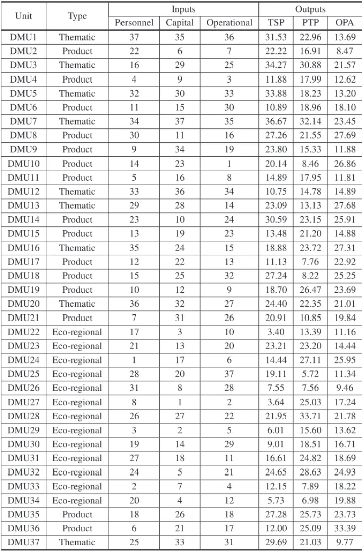
The performance model now in discussion in Embrapa is based on an input oriented DEA-CCR measure, with three inputs and three outputs, computed for each of the 37 research centers. Actually the company comprises 42 research units classified into three types of research-centers: product, eco-regional and thematic. Five of the 42 units were recently created (2010-2012) and were eliminated from the analysis due to lack of data. The centers of the type classification ‘product’ are endeavored to provide feasible solutions in research, development and innovation for specific agricultural products (e.g. soybean, corn and sorghum, cotton, cattle etc.). The eco-regional and thematic centers are concerned, respectively, with research envisaging sustainability of the agriculture in the different Brazilian eco-regions (e.g.: swamplands, savannah etc.) and in basic themes of interest (e.g., satellite monitoring, soil types, informatics and instrumentation for agriculture etc.).
and lends nonparametric properties to the statistical methods based in normality used in the de-termination of weights for the attributes in each performance dimension. The method used is maximum likelihood Factor Analysis. See Souza & Gomes (2015a) for further details about the construction of TSP, PTP and OPA. Table 1 shows the values of the six performance attributes for the year of 2009.
3 DEA AND NON-ARCHIMEDEAN MODELS
3.1 General concepts
Given a set of production units (Decision Making Units-DMUs), with known values for inputs and outputs, the DEA approach aims the calculation of an efficiency measure for each DMU. In general, the efficiency measure is the ratio between two weighted averages of outputs and inputs, respectively. The weights are derived by means of mathematical programming and maximize each DMU performance.
The two most popular DEA models are the CCR and the BCC (Cooper et al., 2007), which differ in the scale assumptions for the efficient frontier: constant returns to scale in the CCR case and variable returns to scale in the BCC case. In the search of the efficient frontier there are two possible radial orientations: input and output orientations. The input orientation is a cost minimization view and the output orientation is a revenue maximization view. The two orientations are equivalent under the constant returns hypothesis, in the sense that they induce the same efficiency measure. The primal (multipliers formulation) DEA-CCR is defined as (1) and the dual (envelope formulation) as (2). Here the production vector of DMUkis (xk,yk), where
xk denotes a r-dimensional input and yk as-dimensional output. The DMU under evaluation has observed production vector (xo, yo). The primal for the DEA-BCC is obtained adding a common scale factor to the objective function and to the inequality restriction in (1). For the envelope DEA-BCC formulation, one must add the restrictionn
k=1λk =1 to (2).
Maxuj,vi s
j=1 ujyoj
s.t.
r
i=1
vixoi =1
−
r
i=1
vixik+ s
j=1
ujykj ≤0, ∀k
uj, vi ≥0, ∀j,i
(1)
Minθ ,λθ
s.t.
θxio− n
k=1
xkiλk ≥0, ∀i
−yoj + n
k=1
ykjλk ≥0,∀j
λk≥0, ∀k
Table 1 – Production observations and types of research centers. Ranks for inputs and weighted average of ranks for outputs.
Unit Type Inputs Outputs
Personnel Capital Operational TSP PTP OPA
DMU1 Thematic 37 35 36 31.53 22.96 13.69
DMU2 Product 22 6 7 22.22 16.91 8.47
DMU3 Thematic 16 29 25 34.27 30.88 21.57
DMU4 Product 4 9 3 11.88 17.99 12.62
DMU5 Thematic 32 30 33 33.88 18.23 13.20
DMU6 Product 11 15 30 10.89 18.96 18.10
DMU7 Thematic 34 37 35 36.67 32.14 23.45
DMU8 Product 30 11 16 27.26 21.55 27.69
DMU9 Product 9 34 19 23.80 15.33 11.88
DMU10 Product 14 23 1 20.14 8.46 26.86
DMU11 Product 5 16 8 14.89 17.95 11.81
DMU12 Thematic 33 36 34 10.75 14.78 14.89
DMU13 Thematic 29 28 14 23.09 13.13 27.68
DMU14 Product 23 10 24 30.59 23.15 25.91
DMU15 Product 13 19 23 13.48 21.20 14.88
DMU16 Thematic 35 24 15 18.88 23.72 27.31
DMU17 Product 12 22 13 11.13 7.76 22.92
DMU18 Product 15 25 32 27.24 8.22 25.25
DMU19 Product 10 12 9 18.70 26.47 23.69
DMU20 Thematic 36 32 27 24.40 22.35 21.01
DMU21 Product 7 31 26 20.91 10.85 19.84
DMU22 Eco-regional 17 3 10 3.40 13.39 11.16
DMU23 Eco-regional 21 13 20 23.21 23.20 14.44
DMU24 Eco-regional 1 17 6 14.44 27.11 25.95
DMU25 Eco-regional 28 20 37 19.11 5.72 11.34
DMU26 Eco-regional 31 8 28 7.55 7.56 9.46
DMU27 Eco-regional 8 1 2 3.64 25.03 17.24
DMU28 Eco-regional 26 27 22 21.95 33.71 21.78
DMU29 Eco-regional 3 2 5 6.01 15.60 13.62
DMU30 Eco-regional 19 14 29 9.01 18.51 16.71
DMU31 Eco-regional 27 18 11 16.61 24.82 18.69
DMU32 Eco-regional 24 5 21 24.65 28.63 24.93
DMU33 Eco-regional 2 7 4 12.15 7.89 18.22
DMU34 Eco-regional 20 4 12 5.73 6.98 19.88
DMU35 Product 18 26 18 27.28 25.73 23.73
DMU36 Product 6 21 17 12.00 25.09 33.39
3.2 Non-Archimedean DEA Models and Assurance Region forǫ(non-Archimedean element)
The classic DEA models may attribute unit efficiency to DMUs that are not efficient in the sense of Pareto-Koopmans (weak efficiency due to the presence of non-null slacks). See Cooper et al. (2007). The necessary and sufficient condition for a DMU to be Pareto-Koopmans efficient is θo=1,uoj >0,vio>0,∀i,j in (1).
One way to impose Pareto-Koopmans efficient solutions is to add the restrictionsuj, vi ≥ε >0,
∀j,ion the weights, whereεdenotes the non-Archimedean positive constant. Thus, the primal model is (3) and the corresponding dual is (4). General DEA models with restrictions on the weights may be seen in Angulo Meza & Lins (2002), Thanassoulis et al. (2004), Portela & Thanassoulis (2006), for instance.
Max s
j=1 ujyoj
s.t. r
i=1
vixio=1
−
r
i=1
vixik+ s
j=1
ujykj ≤0,∀k
uj, vi ≥ε >0, ∀j,i
(3)
Minθo−ε
r
i=1 si−+
s
j=1 sr+
s.t.
θoxio− n
k=1
xikλk−si−=0, ∀i
−yoj + n
k=1
ykjλk−sr+=0, ∀j
λk,si−,sr+≥0, ∀k,i,j
(4)
In general, there is no solution to the problems (3) or (4) without imposing restrictions on the values of the non-Archimedean constant. As discussed in Ali & Seiford (1993b) and in Cooper et al. (2007), it is quite tempting to use a small numerical value forε >0, as 10−5or 10−6, to obtain a solution close to the standard DEA measure. However, the use of very small quantities may lead to numerical problems. Ali (1990) presents a sensitivity analysis using different values ofε >0 and shows the numerical implications in the efficiency calculations. Ali & Seiford (1993a) show that an assurance interval forεis obtained imposing the boundε <1/mink=1...n i=1...rxik. Mehrabian et al. (2000) show that the limit proposed by Ali & Seiford (1993a) is not valid in general and propose a new assurance region. This work is seminal in the area and motivates the approaches of Jahanshahloo & Khodabakhshi (2004), Alirezaee (2005) and MirHassani & Alirezaee (2005).
n being the number of DMUs. In this expressionε∗o(o = 1, . . . ,n)is the solution of (5). The corresponding dual is (6).
Maxεo
s.t.
r
i=1
vixio=1
−
r
i=1
vixki + s
j=1
ujykj ≤0, ∀k
uj ≥εo
vi ≥εo
(5)
Minθo
s.t.
r
i=1 si−+
s
j=1 sr+=1
θoxio− n
k=1
xikλk−si−=0, ∀i
n
k=1
ykjλk−sr+=0, ∀j
λk,si−, sr+≥0, ∀k,i,j
(6)
4 FRACTIONAL REGRESSION
Our aim in this article is the comparison of treatments (groups) in an analysis of variance de-sign with DEA responses. Ramalho et al. (2010) discuss the use of fractional regression models in more general contexts, where a vectorxof contextual variables affects linearly the DEA re-sponse. They consider two modeling alternatives. Here we choose the alternative derived from the model of Papke & Wooldridge (1996) for binary responses. Ifydenotes the DEA response,
x the vector of contextual attributes (in our application a set of group indicator variables), and
G(·)a nonlinear function with values in[0,1], it is postulated thatE(y|x)=G(xθ ). The func-tionG(·) is increasing. Usual choices for G(·) are the logisticG(xθ ) = exθ
1+exθ and G(·) =
(·), where(·)is the inverse of the probability distribution function of the standard normal. In fact, Papke & Wooldridge (1996) suggest as appropriate specification any smooth distribution function.
The fractional regression model postulates that the expected value of the performance measure is a monotonic function of the linear constructµ = xθ. To estimateθ from the observations (xi,yi)i =1, . . .n, one seeksθˆmaximizing the quasi-likelihood function (7).
n
i=1
yilog(G(xiθ ))+(1−yi)log(1−G(xiθ ))
(7)
but not likely to be of importance in our application as emphasized in Gomes et al. (2008). The alternative to this approach is bootstrap.
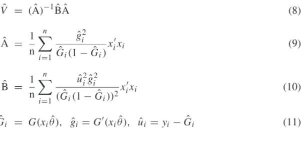
ˆ
V = (Aˆ)−1BˆAˆ (8)
ˆ
A = 1 n
n
i=1
ˆ
gi2
ˆ
Gi(1− ˆGi)
x′ixi (9)
ˆ
B = 1 n
n
i=1
ˆ
u2igˆ2i (Gˆi(1− ˆGi))2
xi′xi (10)
ˆ
Gi = G(xiθ ),ˆ gˆi =G′(xiθ ),ˆ uˆi =yi− ˆGi (11)
5 STATISTICAL RESULTS
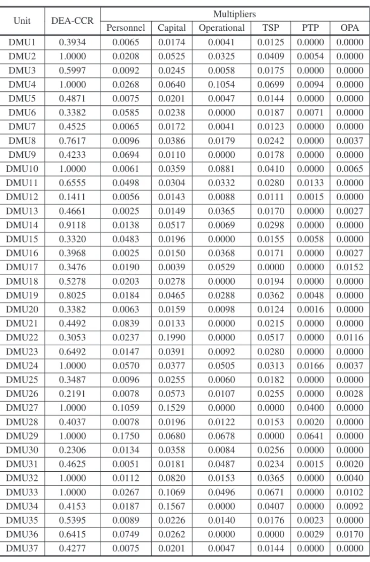
Table 2 shows the standard DEA-CCR scores with the corresponding multipliers (weights). We used the SIAD software (Angulo Meza et al., 2005).
Table 3 shows the non-Archimedean DEA-CCR scores (Perform), as well as the values of the multipliers. The results were obtained via SAS programming, adapting the macro ORDEA of Emrouznejad & Ho (2012).
The performance measurements (Perform) have positive rank correlation of 0.929 with the stan-dard DEA-CCR scores. This shows that inadequacies induced by the non-Archimedean solution are not strong enough to invalidate the analysis. The maximum value of the non-Archimedean constant that can be used is 0.002652, leading to the assurance region interval(0;2.652×10⁻²] (column Epsil in Table 3) and to the measurements Perform. For the non-Archimedean solution the relative weights of labor costs, operational costs and capital are, 19.4%, 24.6% and 56.0%, respectively. These are computed as follows. In Table 2 we computed averages for each input column and measured the relative participation of each column mean. Labor is the relatively cheapest component for the system. In relation to the output components the figures are 66.9%, 20.3% and 12.8% for technical-scientific production, production of technical publications and other activities, respectively. This dictates the direction to improve production efficiency in the company. The shadow price of technical-scientific production dominates the performance score.
Ceteris paribus, DMUs with good technical-scientific production and low values of capital ex-penses will show good performance. Notice that there are no null weights in this solution.
The distribution of Perform is shown in Figure 1 where it is represented a non-parametric estimate of the unknown probability density function. The graph suggests overlapping populations, with a dominating group.
Table 2– Table 2 DEA-CCR scores and multipliers.
Unit DEA-CCR Multipliers
Personnel Capital Operational TSP PTP OPA
DMU1 0.3934 0.0065 0.0174 0.0041 0.0125 0.0000 0.0000
DMU2 1.0000 0.0208 0.0525 0.0325 0.0409 0.0054 0.0000
DMU3 0.5997 0.0092 0.0245 0.0058 0.0175 0.0000 0.0000
DMU4 1.0000 0.0268 0.0640 0.1054 0.0699 0.0094 0.0000
DMU5 0.4871 0.0075 0.0201 0.0047 0.0144 0.0000 0.0000
DMU6 0.3382 0.0585 0.0238 0.0000 0.0187 0.0071 0.0000
DMU7 0.4525 0.0065 0.0172 0.0041 0.0123 0.0000 0.0000
DMU8 0.7617 0.0096 0.0386 0.0179 0.0242 0.0000 0.0037
DMU9 0.4233 0.0694 0.0110 0.0000 0.0178 0.0000 0.0000
DMU10 1.0000 0.0061 0.0359 0.0881 0.0410 0.0000 0.0065
DMU11 0.6555 0.0498 0.0304 0.0332 0.0280 0.0133 0.0000
DMU12 0.1411 0.0056 0.0143 0.0088 0.0111 0.0015 0.0000
DMU13 0.4661 0.0025 0.0149 0.0365 0.0170 0.0000 0.0027
DMU14 0.9118 0.0138 0.0517 0.0069 0.0298 0.0000 0.0000
DMU15 0.3320 0.0483 0.0196 0.0000 0.0155 0.0058 0.0000
DMU16 0.3968 0.0025 0.0150 0.0368 0.0171 0.0000 0.0027
DMU17 0.3476 0.0190 0.0039 0.0529 0.0000 0.0000 0.0152
DMU18 0.5278 0.0203 0.0278 0.0000 0.0194 0.0000 0.0000
DMU19 0.8025 0.0184 0.0465 0.0288 0.0362 0.0048 0.0000
DMU20 0.3382 0.0063 0.0159 0.0098 0.0124 0.0016 0.0000
DMU21 0.4492 0.0839 0.0133 0.0000 0.0215 0.0000 0.0000
DMU22 0.3053 0.0237 0.1990 0.0000 0.0517 0.0000 0.0116
DMU23 0.6492 0.0147 0.0391 0.0092 0.0280 0.0000 0.0000
DMU24 1.0000 0.0570 0.0377 0.0505 0.0313 0.0166 0.0037
DMU25 0.3487 0.0096 0.0255 0.0060 0.0182 0.0000 0.0000
DMU26 0.2191 0.0078 0.0573 0.0107 0.0255 0.0000 0.0028
DMU27 1.0000 0.1059 0.1529 0.0000 0.0000 0.0400 0.0000
DMU28 0.4037 0.0078 0.0196 0.0122 0.0153 0.0020 0.0000
DMU29 1.0000 0.1750 0.0680 0.0678 0.0000 0.0641 0.0000
DMU30 0.2306 0.0134 0.0358 0.0084 0.0256 0.0000 0.0000
DMU31 0.4625 0.0051 0.0181 0.0487 0.0234 0.0015 0.0020
DMU32 1.0000 0.0112 0.0820 0.0153 0.0365 0.0000 0.0040
DMU33 1.0000 0.0267 0.1069 0.0496 0.0671 0.0000 0.0102
DMU34 0.4153 0.0187 0.1567 0.0000 0.0407 0.0000 0.0092
DMU35 0.5395 0.0089 0.0226 0.0140 0.0176 0.0023 0.0000
DMU36 0.6415 0.0749 0.0262 0.0000 0.0000 0.0029 0.0170
Table 3– Non-Archimedean DEA-CCR scores (Perform) and multipliers. Epsil is the marginal non-Archimedean constant.
Unit Perform Multipliers Epsil
Personnel Capital Operational TSP PTP OPA
DMU1 0.1808 0.012208 0.006754 0.008663 0.002653 0.002652 0.002652 0.002652 DMU2 1.0000 0.002652 0.034659 0.104815 0.041984 0.002652 0.002652 0.007173 DMU3 0.4795 0.013266 0.015820 0.013158 0.009934 0.002652 0.002652 0.004364 DMU4 1.0000 0.051966 0.002652 0.256089 0.035665 0.030167 0.002652 0.021248 DMU5 0.2446 0.012533 0.008736 0.010208 0.004759 0.002652 0.002652 0.003017 DMU6 0.3212 0.053722 0.021966 0.002652 0.014425 0.006121 0.002652 0.006061 DMU7 0.2654 0.012302 0.007051 0.009167 0.003218 0.002652 0.002652 0.002739 DMU8 0.6100 0.014349 0.026294 0.017519 0.017584 0.002652 0.002652 0.004579 DMU9 0.3550 0.050960 0.014440 0.002652 0.011886 0.002652 0.002652 0.005261 DMU10 1.0000 0.002652 0.002652 0.901876 0.045008 0.002652 0.002652 0.018031 DMU11 0.6288 0.044632 0.029263 0.038580 0.024551 0.012919 0.002652 0.011124 DMU12 0.1188 0.012388 0.007333 0.009624 0.003734 0.002652 0.002652 0.002820 DMU13 0.3773 0.010405 0.009484 0.030908 0.011657 0.002652 0.002652 0.004107 DMU14 0.6545 0.014287 0.025694 0.017269 0.017146 0.002652 0.002652 0.004768 DMU15 0.3049 0.045189 0.018502 0.002652 0.011694 0.005089 0.002652 0.005454 DMU16 0.3305 0.010493 0.008448 0.028665 0.010336 0.002652 0.002652 0.003714 DMU17 0.3214 0.024246 0.009620 0.038261 0.002652 0.002652 0.011839 0.006505 DMU18 0.3802 0.030752 0.018154 0.002652 0.010698 0.002652 0.002652 0.004340 DMU19 0.7738 0.016711 0.049135 0.027030 0.034269 0.002652 0.002652 0.009435 DMU20 0.2287 0.012519 0.008600 0.010152 0.004660 0.002652 0.002652 0.002981 DMU21 0.3868 0.061583 0.016128 0.002652 0.014607 0.002652 0.002652 0.005573 DMU22 0.2979 0.024096 0.187948 0.002652 0.053425 0.002652 0.007257 0.009032 DMU23 0.5127 0.014377 0.026569 0.017634 0.017786 0.002652 0.002652 0.005125 DMU24 1.0000 0.044055 0.002652 0.151810 0.019357 0.015614 0.011454 0.014816 DMU25 0.1714 0.012794 0.011259 0.011259 0.006602 0.002652 0.002652 0.003326 DMU26 0.1765 0.013186 0.064621 0.002652 0.017390 0.002652 0.002652 0.004290 DMU27 1.0000 0.002652 0.002652 0.488066 0.002652 0.037745 0.002652 0.021783 DMU28 0.3398 0.013102 0.014236 0.012499 0.008777 0.002652 0.002652 0.003842 DMU29 1.0000 0.114346 0.075514 0.101186 0.062761 0.033359 0.007497 0.028381 DMU30 0.2169 0.013800 0.020987 0.015310 0.013708 0.002652 0.002652 0.004591 DMU31 0.4207 0.009952 0.014760 0.042328 0.018384 0.002652 0.002652 0.004933 DMU32 1.0000 0.015005 0.110458 0.004171 0.034807 0.002652 0.002652 0.005894 DMU33 1.0000 0.019026 0.053171 0.147438 0.076629 0.002652 0.002652 0.024939 DMU34 0.3589 0.019140 0.146343 0.002652 0.042619 0.002652 0.004826 0.007436 DMU35 0.4659 0.013596 0.019018 0.014489 0.012269 0.002652 0.002652 0.004811 DMU36 0.6149 0.069804 0.025528 0.002652 0.002652 0.003714 0.014674 0.007634 DMU37 0.2596 0.012708 0.010425 0.010912 0.005993 0.002652 0.002652 0.003329
The formal statistical analysis with quasi-maximum likelihood estimation confirms the impres-sion conveyed by Figures 1 and 2. The model was fitted with the logistic distribution func-tion, with the mean value of the response variable dependent of the linear construct µi = b0+b1di1+b2di2. In this expression, the variablesdi1anddi2are indicators of the types
Figure 1– Density probability function for the non-Archimedean measure.
Figure 2– Box plots for the non-Archimedean measure by DMU type.
b = (b0,b1,b2)is given bybˆ = (0.4811,0.1324,−0.8395), indicating the low performance
of the thematic centers. The variance-covariance matrixV is estimated by
ˆ
V =
⎛
⎜ ⎝
0.1679529 −0.167953 −0.167953
−0.167953 0.2520028 0.1679529
−0.167953 0.1679529 0.221968
⎞
The joint significance ofb=(b0,b1,b2)is assessed using the statisticl= ˆb(Vˆ)−1bˆ′, distributed
as the qui-square with three degrees of freedom under the hypothesisb=0. We havel=8.234, withp-value of 0.041. The pairwise differences between the types thematic and product, product and eco-regional, and thematic and eco-regional are assessed using estimates of the quantities
b1−b2,b1,b2, respectively. The test statistics are
z1= buˆ ′ 1
u1V uˆ ′1
, z2= buˆ ′ 2
u2V uˆ ′2
and z3= buˆ ′ 3
u3V uˆ ′3
,
whereu1=(0,1,−1),u2=(0,1,0)andu3=(0,0,1), respectively. Under the null hypotheses
of no differences they are distributed as the standard normal. We havez1=2.616,z2=0.264,
z3 = −1.782 with p-values 0.009, 0.792 and 0.075, respectively. The statistics indicate the dominance of the type product over thematic. The difference between types thematic and eco-regional is only marginally significant.
6 SUMMARY AND FINAL CONSIDERATIONS
In this article we used a DEA-CCR model with a non-Archimedean constantε >0 to compute performance measurements for 37 research centers of the Brazilian Agricultural Research Corpo-ration. The model is based on a three dimensional output vector, constructed from the observed ranks of several production variables grouped into three performance categories: technical-scientific publications, technical publications, and other production activities. The input vec-tor is defined by ranks on labor expenses, operational costs, and capital expenses. All produc-tion variables were previously normalized by the DMU labor quantity. An effort was made to use a weighting system not involving management pre-judgments. This was achieved via Factor Analysis.
The motivation for the non-Archimedean approach was dictated by the interest to obtain a weight distribution indicating usage of all input and output components. In this context, efficient units are Pareto-Koopmans efficient. The non-Archimedean ε was chosen as the upper limit of the assurance region proposed in Mehrabian et al. (2000).
between publications and other activities. The outputs shadow prices may be used as weights in a goal evaluation system where actual production is compared with target production.
The distribution of the non-Archimedean DEA-CCR suggests overlapping of populations and dominance of research centers of the product type. This impression is confirmed by box plots. Median performances for the three types of research centers studied – product, eco-regional and thematic – are 0.610, 0.421 and 0.260, respectively. The types of research centers were further compared with the use of fractional regression and quasi-maximum likelihood estimation. Formal statistical methods confirm, in part, the descriptive statistics results. The product research centers dominate thematic, and the thematic centers marginally dominate the eco-regional. It should be noticed that the distribution of output intensity for units’ types is [69.0%, 20.9%, 10.1%] for eco-regional, [67.1%, 19.1%, 13.8%] for product and [54.4%, 22.8%, 22.8%] for thematic, for TSP, PTP and OPA, respectively. These figures explain the low performance on the median of thematic units and corroborates the general indication suggested by the medians that research centers with high levels of TSP tend to show good performance. The same effect is not captured by the regression model due to the high variation of the efficiency measurements for eco-regional centers.
REFERENCES
[1] ALIAI & SEIFORDLM. 1993b. The mathematical programming approach to efficiency analysis. In: The Measurement of Productive Efficiency: Techniques and Applications [edited by FRIEDHO, LOVELLCAK & SCHMIDTSS], Oxford University Press, 120–159.
[2] ALIAI & SEIFORDLM. 1993a. Computational accuracy and infinitesimals in data envelopment analysis.INFOR,31(4): 290–297.
[3] ALIAI. 1990. Data Envelopment Analysis – Computational Issues.Computers, Environment and Urban Systems,14: 157–165.
[4] ALIREZAEE MR. 2005. The overall assurance interval for the non-archimedean epsilon in DEA models: A partition base algorithm.Applied Mathematics and Computation,164(3): 667–674.
[5] ANGULOMEZA L & LINSMPE. 2002. Review of methods for increasing discrimination in data envelopment analysis.Annals of Operations Research,116: 225–242.
[6] ANGULOMEZAL, BIONDINETOL, SOARES DEMELLO JCCB & GOMESEG. 2005. ISYDS – Integrated System for Decision Support (SIAD – Sistema Integrado de Apoio `a Decis˜ao): a software package for Data Envelopment Analysis model.Pesquisa Operacional,25(3): 493–503.
[7] AVILAAFD, GOMESEG, SOUZAGS, PENTEADOFILHORC & SOUZAMO. 2013. Avaliac¸˜ao de desempenho de unidades de pesquisa agropecu´aria: m´etricas e resultados da experiˆencia da Embrapa. Documentos, 16, Embrapa, Bras´ılia, DF, Brasil.
[8] B ˘ADINL, DARAIOC & SIMARL. 2012. How to measure the impact of environmental factors in a nonparametric production model.European Journal of Operational Research,223(3): 818–833.
[10] COOPERWW, SEIFORDLM & TONEK. 2007. Data Envelopment Analysis: A Comprehensive Text with Models, Applications, References and DEA-Solver Software. 2nd Ed. New York: Springer.
[11] EMROUZNEJADA & HOW. 2012. Applied Operational Research with SAS. New York: CRC Press.
[12] GOMESEG, SOUZAGS & VIVALDILJ. 2008. Two-stage inference in experimental design using DEA: an application to intercropping and evidence from randomization theory.Pesquisa Operacional, 28: 339–354.
[13] JAHANSHAHLOO GR & KHODABAKHSHI M. 2004. Determining assurance interval for non-archimedean element in the improving outputs model in DEA.Applied Mathematics and Compu-tation,151(2): 501–506.
[14] MEHRABIANS, JAHANSHAHLOOGR, ALIREZAEEMR & AMINGR. 2000. An assurance interval for the non-Archimedean epsilon in DEA models.Operations Research,48(2): 344–347.
[15] MIRHASSANISA & ALIREZAEEMR. 2005. An efficient approach for computing non-archimedean epsilon in DEA based on integrated models.Applied Mathematics and Computation,166(2): 449– 456.
[16] OLESEN OB, PETERSENNC & PODINOVSKVV. 2015. Efficiency analysis with ratio measures.
European Journal of Operational Research,245: 446–462.
[17] PAPKELE & WOOLDRIDGEJM. 1996. Econometric methods for fractional response variables with an application to 401(k) plan participation rates.Journal of Applied Economics,11(6): 619–632.
[18] PORTELAMCAS & THANASSOULISE. 2006. Zero weights and non-zero slacks: Different solutions to the same problem.Annals of Operations Research,145(1): 129–147.
[19] RAMALHOEA, RAMALHOJJS & HENRIQUESPD. 2010. Fractional regression models for second stage DEA efficiency analyses.Journal of Productivity Analysis,34: 239–255.
[20] SIMARL & WILSONPW. 2007. Estimation and inference in two-stage, semi-parametric models of production processes.Journal of Econometrics,136(1): 31–64.
[21] SIMARL & WILSONPW. 2011. Two-stage DEA: caveat emptor.Journal of Productivity Analysis, 36: 205–218.
[22] SOUZAGS & GOMESEG. 2015a. Performance measure to support decision-making in agricultural research centers in Brazil.Procedia Computer Science,55: 405–414.
[23] SOUZAGS & GOMESEG. 2015b. Management of agricultural research centers in Brazil: A DEA application using a dynamic GMM approach.European Journal of Operational Research, 240: 819–824.
[24] SOUZA GS, AVILAAFD & ALVESER. 1999. Technical efficiency of production in agricultural research.Scientometrics,46(1): 141–160.
[25] THANASSOULISE, PORTELAMCAS & ALLENR. 2004. Incorporating value judgments in DEA. In: Handbook on Data Envelopment Analysis [edited by COOPERWW, SEIFORDLM & ZHUJ],