Spatial distribution of top soil water content in an experimental
catchment of Southeast Brazil
Carlos Rogério de Mello
1*; Léo Fernandes Ávila
1; Lloyd Darrell Norton
2; Antônio Marciano
da Silva
1;
José Márcio de Mello
3; Samuel Beskow
41
UFLA – Depto. de Engenharia, C.P. 3037 – 37200-000 – Lavras, MG – Brasil. 2
USDA/ARS – National Soil Erosion Research Laboratory, Purdue University, 275 South Russell Street – 47907-2077 – West Lafayette, IN, USA.
3
UFLA – Depto. de Ciências Florestais. 4
UFPel – Centro de Desenvolvimento Tecnológico/Engenharia Hídrica – 96060-290 – Pelotas, RS – Brasil. *Corresponding author <[email protected]>
ABSTRACT:Soil water content is essential to understand the hydrological cycle. It controls the surface runoff generation, water infiltration, soil evaporation and plant transpiration. This work aims to analyze the spatial distribution of top soil water content and to characterize the spatial mean and standard deviation of top soil water content over time in an experimental catchment located in the Mantiqueira Range region, state of Minas Gerais, Brazil. Measurements of top soil water content were carried out every 15 days, between May/2007 and May/2008. Using time-domain reflectometry (TDR) equipment, 69 points were sampled in the top 0.2 m of the soil profile. Geostatistical procedures were applied in all steps of the study. First, the spatial continuity was evaluated, and the experimental semi-variogram was modeled. For the development of top soil water content maps over time a co-kriging procedure was used having the slope as a secondary variable. Rainfall regime controlled the top soil water content during the wet season. Land use was also another fundamental local factor. The spatial standard deviation had low values under dry conditions, and high values under wet conditions. Thus, more variability occurs under wet conditions.
Key words:Mantiqueira Range, soil water content mapping, soil hydrology, geostatistical techniques
Distribuição espacial da umidade superficial do solo em uma bacia
hidrográfica experimental do Sudeste do Brasil
RESUMO:A umidade do solo é essencial para o entendimento do ciclo hidrológico, uma vez que controla a geração do escoamento superficial, infiltração de água no solo, evaporação do solo e transpiração das plantas. Este trabalho objetivou analisar os padrões espaciais da umidade superficial do solo e caracterizar a média e o desvio padrão espaciais da mesma ao longo do tempo em uma bacia hidrográfica experimental localizada na Serra da Mantiqueira, MG. As medidas da umidade superficial do solo foram conduzidas a cada 15 dias, entre Maio/2007 e Maio/2008, usando um equipamento TDR portátil, em 69 pontos amostrados na camada de 0-20 cm. Procedimentos geoestatísticos foram aplicados em todas as etapas do trabalho. Primeiramente, a continuidade espacial foi avaliada modelando-se o semivariograma experimental. Mapas de umidade do solo foram desenvolvidos com base na co-krigagem usando o padrão de declividade como variável secundária. O regime de chuvas controlou a umidade superficial do solo durante o período úmido, devido aos altos conteúdos de umidade. O uso do solo também foi outro fator fundamental na distribuição espacial da umidade do solo. O desvio padrão espacial apresentou baixos valores sob condições secas e valores mais altos sob condições úmidas.
Palavras-chave:Serra da Mantiqueira, mapeamento do solo, hidrologia do solo, técnicas geoestatísticas
Introduction
Soil water content is one of the main hydrological cycle elements. It controls the surface runoff generation, soil wa-ter infiltration, soil evaporation and plant transpiration. Its spatial distribution has received special attention to help to identify areas that are more susceptible to surface runoff and sediment transport (Western et al., 2004; Hébrard et al., 2006; Mahanama et al., 2008). At the catchment scale, the concern is mainly on understanding the environmental balance and impacts due to land-use change and soil tillage on surface runoff and erosion processes.
The Mantiqueira Range is an important water produc-ing region in south-east Brazil. Atlantic Forest is the most
from remote sensing techniques (Western et al., 2004; Brocca et al., 2008).
Geostatistical techniques have been applied to study the spatial variability of top soil water content (Western et al., 2004; Hébrard et al., 2006; Brocca et al., 2007; Zhu and Shao, 2008). To proceed with geostatistical mapping, it is impera-tive that a consistent study of the spatial continuity be car-ried out using semi-variogram modeling procedures (Isaaks and Srivastava, 1989; Western et al., 2004; Diggle and Ribeiro Júnior, 2007).
Based on this context, we investigated: i) the spatial dis-tribution of top soil water content using a geostatistical ap-proach in an experimental headwater catchment located in the Mantiqueira Range, southeast Brazil; and ii) the spatial mean and standard deviation of the top soil water content in dif-ferent land use sites over the time, applying a simulation kriging technique.
Material and Methods
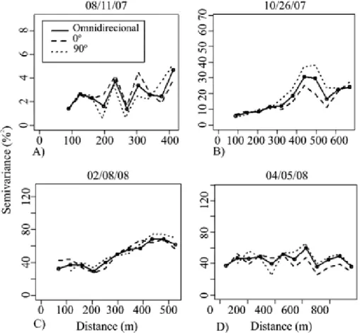
The Lavrinha Creek Experimental Catchment (LCEC) consists of an experimental area in which many hydrologic, climatic and pedologic investigations have been carried out since 2004. It is located in the Mantiqueira Range region which is the most important water divisor in southeast Brazil, at the border between the States of São Paulo, Minas Gerais and Rio de Janeiro (Figure 1). This region is extremely im-portant for southeast Brazil in terms of water yield, being responsible for a significant part of the Brazilian
hydroelec-tric energy production. The LCEC has 6.87 km2 of drainage area, its altitude ranges from 1,159 m to 1,713 m and the mean slope is 35%. The Köppen Climate Classification is Cwb, which is characterized by the concentration of rainfall during summer (October-March). The winter is cold and dry and the annual mean temperature is 15o
C, ranging from 9o
C (mean of the winter) to 19oC (mean of the summer). The annual mean rainfall is 1,950 mm, 80% occurring in sum-mer (Mello et al., 2008).
The Digital Elevation Model (DEM) and the soil map are presented in Figure 2a and 2b, respectively. Soils were clas-sified by Menezes et al. (2009) as Fluvic Neosol, occupying 7.1% of the area, Haplic Gleisol 0.9% and Haplic Cambisol 92% of the catchment. The Cambisol occupies the steepest areas and is located at a higher altitude. It comprises shallow soils (up to 1.0 m), with low water holding capacity and in-filtration restriction caused by surface crusting, mainly in bare areas, due to the high fine silt concentration (Menezes et al., 2009). The Fluvic Neosol is located on the outlet of the catch-ment, following the Lavrinha Creek channel and presents a deeper soil layer than the Cambisol and a water table that is near the surface most of the year. The Haplic Gleisol
occu-Figure 1 – Location of the Lavrinha Creek Experimental Catchment (LCEC).
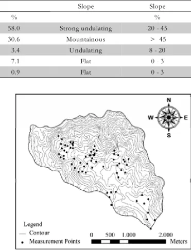
pies a very limited proportion of the catchment to be taken into considereation for top soil water content monitoring. The soil classifications as well as their distribution and relief conditions (Table 1) show that more than 88% of the catch-ment presents slopes greater than 20% and, approximately, 11% of area has slopes above 45%.
The LCEC’s land-use map was generated by remote sens-ing procedures ussens-ing a high resolution satellite “Alos” im-age of May/2008 (10 m of resolution) (Figure 3). Ground validation was carried out. Atlantic Forest and Forest Regen-erated (more than 20 years old) cover, respectively, 284.8 ha (41.5%) and 90.0 ha (13.2%) of the area, followed by planted grassland of 277.8 ha (40.4%) and native wetland pasture is 33.5 ha (4.9%). Land-use distribution is extremely impor-tant in the context of spatial distribution of soil water con-tent, therefore, it needs to be adequately mapped, especially under subtropical mountainous conditions like the Mantiqueira Range (Western et al., 2004).
Soil water content can be measured by using water con-tent sensors such as time domain reflectometers - TDR (Souza and Folegatti, 2010). In this study, the volumetric soil water content was measured over the top 0.20 m of the soil profile using a portable TDR probe unit of the IMKO, Trime – FM model. This equipment was previously calibrated for each soil and land use, based on the gravimetric method for determination of soil water content and bulk density as
ref-erence (Western et al., 2004). A second degree polynomial equation was fit, presenting a coefficient of determination of 0.91 for Atlantic Forest and grassland sites, and 0.86 for the wetland site.
Due to the predominance of the Haplic Cambisol in the catchment as well as slopes greater than 20% in almost 90% of the catchment (Table 1), the definition of sample distri-bution was carried out having the land-use as reference, be-cause this physiographic characteristic is responsible for a greater variability of soil water content than the pedologic and topographic attributes under the environmental condi-tions of this catchment.
Top soil water content was monitored at 69 measure-ment points (Figure 4) over the land uses (15 in the Atlantic Forest Regeneration site, 8 in the Wetland site, 22 in the At-lantic Forest site and 24 in the Grassland), every 15 days, with support of a high precision GPS. This sampling procedure is similar to that adopted by Bárdossy and Lehmann (1998) and Zhu and Shao (2008) who worked, respectively, with 60 points in a catchment of 6.3 km2
and 37 points in a catch-ment of 6.89 km2
.
Exploratory analyzes were applied to each data set of the soil water content. Outliers were identified and then removed based on box plot graphs (Diggle and Ribeiro Júnior, 2007). Evaluation of the top soil water content distribution in func-tion of the latitude and longitude allows verifying whether
Table 1 – Catchment area occupied with respective topographic conditions.
Soil Area Slope Slope
ha % %
H aplic C ambisol 398.8 58.0 Strong undulating 20 - 45
H aplic C ambisol 210.0 30.6 Mountainous > 45
H aplic C ambisol 23.8 3.4 U ndulating 8 - 20
Fluvic N eosol 48.6 7.1 Flat 0 - 3
H aplic Gleisol 5.8 0.9 Flat 0 - 3
Figure 3 – Land use map of the Lavrinha Creek Experimental Catchment (LCEC).
the data sets present bias. For this, graphs relating soil water content with geographical coordinates were created. When soil water content presented a significant correlation with the lati-tude or longilati-tude, the data set was characterized as biased. This bias needs to be removed so that the geoestatistic pro-cedures can be applied (Isaaks and Srivastava, 1989). This test is very important to characterize the spatial dependence of any geo-referenced variable. If some data set presents bias in some direction, the spatial dependence can be over charac-terized, thus compromising the geostatistical intrinsic hypoth-esis (Isaaks and Srivastava, 1989). In several scientific stud-ies, where geostatistical techniques were applied, both outli-ers and bias effects have been neglected.
Geostatistical analyses were carried out to assess the spa-tial distribution of top soil water content. A semivariogram model was fitted to the experimental semivariogram. Expo-nential, Spherical and Gaussian semivariogram models were evaluated (Isaaks and Srivastava, 1989). For model fitting, Maximum Likelihood, Weighted Minimum Square and Or-dinary Minimum Square methods were tested (Diggle and Ribeiro Júnior, 2007). Statistical coefficients of precision were used to determine the best models which were calculated based on the results obtained from a cross-validation method. This method is a traditional geostatistical procedure for validation. Basically, it consists on the removal of each one of the points that were sampled, structuring a new sam-pling. Afterwards, the semi-variogram model is re-fitted for this new sampling and applied to estimate, by ordinary kriging, the value for the removed point and then it is com-pared to the observed value, producing an error estimate. This procedure is repeated for all the sampled points, thus a statistical precision can be obtained (Cressi, 1993). The sta-tistical coefficients were the Reduced Mean Error – RME (eq.1) and the Standard Deviation of the Reduced Error – SER (eq.2).
(
)
(
)
n
obsi esti
i 1 esti
Z Z
1 RME
n = Z
− = ⋅
σ
∑
(1)in which n is the number of observations; Zobsi corresponds to the soil water content observed at point i; Zesti is the soil water content estimated by kriging (from cross-validation) at same point i; σ (Zesti) is the standard deviation of the es-timates.
(
)
n
obsi esti ER
i 1 esti
Z Z
1 S
n = Z
−
= ⋅
σ
∑
(2)Besides these statistical precision tests, the semi-variogram models were also evaluated considering the Spa-tial Dependence Degree (SDD), whose definition was adapted from the concept developed by Cambardella et al. (1994):
( )
11 0
C
SDD % 100
C C
⎛ ⎞
=⎜ + ⎟⋅
⎝ ⎠ (3)
SDD means how much of the variance is explained by the spatial dependence structure and it is calculated on the
basis of semi-variogram model parameters; C1 corresponds to the structured variance; C0 is the nugget effect and (C1 + C0) is known as either sill or contribution to the spatial de-pendence (Isaaks and Srivastava, 1989). SDD is often ana-lyzed according to ranges: less than 25%, the semi-variogram model presents a low spatial dependence degree; between 25 and 75%, moderate spatial dependence degree and greater than 75%, strong spatial dependence degree (Cambardella et al., 1994).
Another important analysis of data sets corresponds to anisotropy. It means that the spatial variability can present different behavior in some specific geographical direction. The anisotropy can be studied by comparison of the experimen-tal semi-variogram plotted in a specific direction (known as directional semi-variogram) to the isotropic experimental semi-variogram (Isaaks and Srivastava, 1989; Diggle and Ribeiro Júnior, 2007). The evaluated directions were 0o
and 90o, corresponding to East-West and North-South directions, respectively. To figure out if there was anisotropy, a visual evaluation was made, observing the characteristics of the di-rectional semi-variograms in comparison to the isotropic semi-variogram, especially, in the range and nugget effect (Western et al., 2004; Brocca et al., 2008).
After semi-variogram modeling, ordinary co-kriging was applied to mapp the top soil water content over the moni-tored period based on the best fitted semi-variogram model. The co-kriging estimates a variable (in this case, top soil wa-ter content - Z) at a location i, using n observations of the same variable (z1) in the neighborhood and m observations of the secondary variable (z2) at a location k. The secondary variable is easier to obtain (under field conditions and through the application of some GIS procedures) than the main variable and is co-related with it. In this case, the slopes were computed based on the Digital Elevation Model (DEM), thus creating a slope class map. The general equation for co-kriging is:
(
)
(
)
n m
i 1j 1j 2k 2k
j 1 k 1
Z z z
= =
=
∑
⋅ λ +∑
⋅ λ (4)The use of the co-kriging method to generate a soil wa-ter content maps is based on the existence of a second vari-able (slope, for instance), which is more commonly availvari-able than soil water content (primary variable). The latter variable was obtained having the land-use as reference; nevertheless, some areas of the catchment were not adequately sampled because of the great difficulty in accessibility of sites with dense forest and very strong slopes. In this kind of situa-tion, the co-kriging procedure can help to reduce error esti-mates where there are fewer samples with the use of a sec-ond variable which presents a high correlation with the pri-mary variable since the slopes influence water movement and distribution in the soil profile.
con-sists of numerical block kriging and is positioned in the best fitted semi-variogram model, reproducing the random func-tion characterized by each dataset. The simulafunc-tion kriging pro-cedure consists of the application of the Monte Carlo Method in which 5000 realizations were generated for each site. These realizations are completely randomized in terms of the points allocated on sites, generating both spatial mean and standard deviation from the kriging interpolations on these 5000 realizations, considering a confidence interval for spatial mean of 95%. This procedure was also applied by Mello et al. (2009) in their studies on estimates of volumes of eucalyptus plantations, obtaining good results in terms of precision.
Results and Discussion
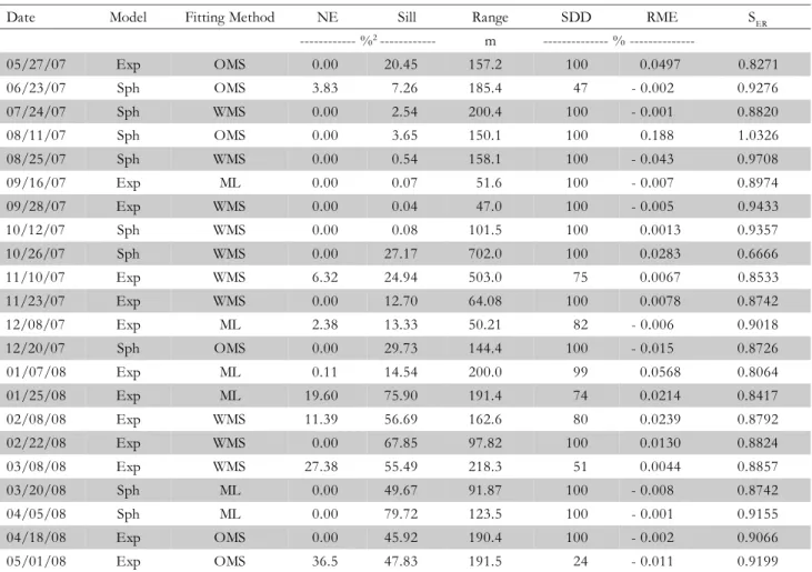
Experimental semi-variograms were plotted in directions East-West (0o) and North-South (90o) in the LCEC (Figure 5), and respective experimental isotropic semi-variogram (uni-directional semivariogram). The range of semi-variograms, in both directions, is similar to the range of unidirectional experimental semi-variogram, with values between 50 and 200 m. In addition, the general behavior of semi-variograms in 0o and 90o directions is similar to the unidirectional semi-variogram, especially, for distances smaller than the range of the semivariogram. In other words, there is no difference be-tween anisotropic and isotropic semi-variograms in the
dis-tance which geostatistical procedures can be applied (p < 0.05) Brocca et al. (2007) made the same observation about the behavior of spatial continuity of top soil water content in a small catchment in Italy and concluded that there is no dif-ference between the experimental semi-variograms on E-W and N-S directions and unidirectional semi-variogram. Thus, based on these observations and results, the semi-variogram modeling was carried out considering only the unidirectional semi-variogram.
The best unidirectional semi-variogram model is shown for each date and respective of fitting method and estimated parameters, statistics of precision and spatial dependence de-gree (Table 2). The exponential model demonstrated a bet-ter performance in 13 of the 22 evaluated data sets. The spherical model was the best in nine situations. The Gaussian model was tested in all situations and good re-sults were found. However, the precision of these fittings was not as good as those of previously mentioned models. These results show the relevance of the test of semi-variogram models and the fitting methods, although the ex-ponential model has presented better performance (in 59% of situations) and has been applied in many other studies. Conversely, Western et al. (2004) verified that the exponen-tial model did not produce satisfactory performance to de-scribe the spatial continuity of top soil water content in one of the sites studied by them, using a similar approach as in this work.
The spatial dependence degree (SDD) allowed verifying the magnitude of the spatial continuity of the top soil water con-tent, being the smallest value greater than 25%. Predominantly, SDD was greater than 75% (in 17 cases), characterizing a strong spatial dependence degree (Cambardella et al., 1994). The top soil water content presents relevant spatial dependence degree which is essential for studying the spatial variability patterns based on geostatistical procedures. Evaluating this same as-pect, Brocca et al. (2007) found a good fit for the spatial dis-tribution of the top soil water content with the exponential semi-variogram.
Figure 6 presents the semi-variogram fitted to the experi-mental semi-variogram, grouped according to the season of year. The fitting quality can also be usually evaluated by the scattering of points around the model curve. For the data sets of 06/23/2007, 05/01/2008 and 03/08/2008, the semi-variograms presented inferior quality (low spatial dependence degree – Table 2). For the dates 07/24/07, 08/11/2007, 10/ 12/2007 and 04/18/2008, the fitting of semi-variograms should be evaluated carefully. The OMS and WMS fitting meth-ods, which were chosen for these data sets, can underestimate the nugget effect due to the uncertainty associated to the small sampling scale that was adopted, producing values of SDD greater than the expected values. Nevertheless, the graphs in Figure 6 demonstrate better the spatial continuity of the top
soil water content under wet conditions (October – March), observed nugget effects and sill are better characterized than the fittings obtained under dry conditions. Brocca et al. (2007) found similar results for conditions of a catchment in Italy. The authors mentioned that during the wet season, the top soil water content presented a more structured spatial conti-nuity than during the dry season. This same aspect also was obtained by Grayson et al. (1997), showing the importance of the local hydrologic conditions in soil water content distribu-tion. During the wet season, the weather conditions exert a predominant influence on the top soil water content spatial continuity (Figure 6), although the topographic conditions are important in controlling water movement and consequently the spatial continuity pattern (Grayson et al., 1997).
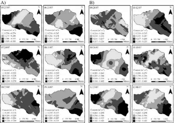
The top soil water content maps were clustered into two groups, following the season of the year. Figures 7 and 8 present the co-kriging maps generated by the application of a secondary variable (slope). Figure 7a presents the winter maps (from May, 27 to September, 16). A decrease of the top soil water content can be observed, varying from 0.33 m3 m–3 (33%) (in May) to 0.21 m3
m–3
(21%) (in September) as a consequence of the dry season. In areas near to the outlet of the catch-ment (having flatter slope), the top soil water content is greater than in other sites. This pattern occurs due to the soil water movement from the highest sites in the catchment into the Table 2 – Semi-variogram model parameters, Spatial Dependence Degree (SDD) and statistics of precision obtained for
each data set of top soil water content in the LCEC between May/2007 and May/2008.
Date Model Fitting Method NE Sill Range SDD RME SER
--- %2 --- m %
---05/27/07 Exp OMS 0.00 20.45 157.2 100 0.0497 0.8271
06/23/07 Sph OMS 3.83 7.26 185.4 47 - 0.002 0.9276
07/24/07 Sph WMS 0.00 2.54 200.4 100 - 0.001 0.8820
08/11/07 Sph OMS 0.00 3.65 150.1 100 0.188 1.0326
08/25/07 Sph WMS 0.00 0.54 158.1 100 - 0.043 0.9708
09/16/07 Exp ML 0.00 0.07 51.6 100 - 0.007 0.8974
09/28/07 Exp WMS 0.00 0.04 47.0 100 - 0.005 0.9433
10/12/07 Sph WMS 0.00 0.08 101.5 100 0.0013 0.9357
10/26/07 Sph WMS 0.00 27.17 702.0 100 0.0283 0.6666
11/10/07 Exp WMS 6.32 24.94 503.0 75 0.0067 0.8533
11/23/07 Exp WMS 0.00 12.70 64.08 100 0.0078 0.8742
12/08/07 Exp ML 2.38 13.33 50.21 82 - 0.006 0.9018
12/20/07 Sph OMS 0.00 29.73 144.4 100 - 0.015 0.8726
01/07/08 Exp ML 0.11 14.54 200.0 99 0.0568 0.8064
01/25/08 Exp ML 19.60 75.90 191.4 74 0.0214 0.8417
02/08/08 Exp WMS 11.39 56.69 162.6 80 0.0239 0.8792
02/22/08 Exp WMS 0.00 67.85 97.82 100 0.0130 0.8824
03/08/08 Exp WMS 27.38 55.49 218.3 51 0.0044 0.8857
03/20/08 Sph ML 0.00 49.67 91.87 100 - 0.008 0.8742
04/05/08 Sph ML 0.00 79.72 123.5 100 - 0.001 0.9155
04/18/08 Exp OMS 0.00 45.92 190.4 100 - 0.002 0.9066
wetlands (on this site, the water movement is constrained due to the flat slope). The northern part of the catchment which is covered by Atlantic Forest (Figure 3) has the least variability of top soil water content throughout the winter. This behav-ior is associated with the characteristics of the Atlantic Forest in the Mantiqueira Range, presenting up to 50-cm litter layer, low values of soil bulk density (< 600 kg m–3), high organic matter concentration (> 0.09 kg kg–1
) and the highest values of both saturated hydraulic conductivity and drainable
poros-ity (Junqueira Júnior et al., 2008). All of these soil physical attributes under Atlantic Forest play a fundamental role in the attenuation of top soil water content fluctuations through-out the year.
In grassland sites, there are greater top soil water contents than in the forest sites, especially, in July and August. This top soil water content distribution can be explained by the occurrence of rare rainfall events, characterized by low inten-sity during winter. The soils in grassland sites are more af-Figure 6 – Semi-variograms fitted for each data set measured according with the season of year (A – winter; B – spring; C – summer; D –
Figure 7 –Top soil water content maps associated with the winter (A) and spring (B) generated by co-kriging applying the slope as secondary variable.
Figure 8 – Top soil water content maps associated with the summer (A) and autumn (B) generated by co-kriging applying the slope as secondary variable.
fected by rain than the soils under Atlantic Forest sites due to the low Leaf Area Index (produced by weak grassland un-der the dry condition) and consequently no rainfall interceptation by the canopy.
The greatest top soil water content during the year (greater than 0.40 m3
m–3
ca-pacity which is around 0.35 m3m–3 for LCEC soils (Junqueira Júnior et al., 2008). By comparing the top soil water content co-kriging maps linked to the land-use map (Figure 3), it is possible to observe that in January and February occurs a greater reduction of top soil water content in grassland sites (due to the non-occurrence of rainfall during 15 consecutive days). The root system of the grassland is responsible for this behavior because the effective roots are concentrated in the first 0.2 m and, in summer, the evapotranspiration is maximized by weather conditions.
At the beginning of autumn (Figure 8b), the top soil water content in the Atlantic Forest sites is greater than the other sites, basically due to the good physical quality of soils (better soil particle distribution and also greater porosity, satu-rated hydraulic conductivity, organic matter concentration). All of these features affect positively the soil water holding effi-ciency and lateral water redistribution on these sites when compared to grassland sites (Qiu et al., 2001). Under wet con-ditions, there is greater correlation between porosity and hy-draulic conductivity, with lateral water redistribution one of the most important local factors that control the soil water content in top soil (Famiglietti et al., 1998). The maps on Figure 8b also demonstrate a reduction in the top soil water content values in grassland sites since the changes in these sites are faster than in other sites, especially in Wetlands.
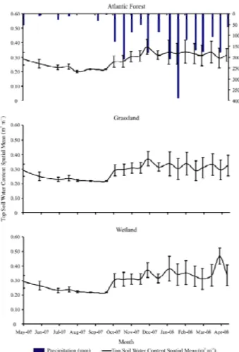
The top soil water content for grassland sites, specifically in the west of the LCEC, presented the least values. This behavior can be associated with the sloping slope which pro-motes water movement to the downstream areas. The com-bination of both factors (grassland and sloped slope) deter-mines the soil water content regime in this area during the dry season. The mean spatial top soil water content at each site (Atlantic Forest, Grassland and Wetland) and respective standard deviations (Figure 9) had a depletion of soil water content at all sites (from May to September) (p < 0.05). How-ever, the reduction was less pronounced at wetland sites due to the water redistribution from the upper areas. After Oc-tober, an increase of soil water content can be noticed, con-sidering the same confidence interval for spatial mean, espe-cially for the grassland sites, because the rainfall is less inter-cepted by this type of vegetation (p < 0.05).
A seasonal evolution of the standard deviation at all sites (Figure 9) was observed as a result of specific weather con-ditions of the region (dry winter and wet summer). This behavior indicates that the spatial patterns of the top soil water content are predominantly controlled by summer weather characteristics. Nevertheless, the local conditions, such as land use and slope, exert control on the soil water con-tent, especially, during the dry season. Western et al. (2004) worked in catchments in Australia and New Zealand, in a similar situation, concluding that the wet conditions in catchments determine the spatial distribution of soil water content, with local factors being also important, especially the slope.
The standard deviations indicate that the top soil water content had high variability during the wet season. This be-havior can be explained by soil hydrologic attributes. Dur-ing the occurrence of rainfall, the infiltration process occurs,
Figure 9 – Mean temporal spatial top soil water content and respective standard deviation on the land-use sites in the Lavrinha Creek Experimental Catchment (LCEC) generated by simulation kriging.
being strongly influenced by the hydraulic conductivity which is related to the land use in LCEC (Menezes et al., 2009).
This result can be important to support satellite image interpretation to extract an indicator of the soil water con-tent distribution based on remote sensing methods, espe-cially in regions with a high concentration of rainfall, diverse land use, and slope that is mountainous and strongly un-dulated, such as the Mantiqueira Range region. Furthermore, recent attention has been given to the calibration of hydro-logic models using antecedent soil water content mapping obtained from remote sensing analyses (Brocca et al., 2008; Koren et al., 2008; Mahanama et al., 2008). One of the con-tributions of this study was to demonstrate how the mean spatial top soil water content obtained through simulation kriging can be used to estimate soil water content, and thus reduce the processing time as well as improve the perfor-mance of the models.
Conclusions
con-tent, and the land use was an important local factor in this season. The spatial standard deviation of top soil water con-tent in all sites presents lower values during the dry season. However, there is a larger spatial variability as the wet season begins. To ensure better monitoring of the top soil water content over time, it is imperative to increase the number of samples during the wet season. Simulation kriging was efficient and can assist in the development of remote sens-ing procedures to identify the soil water content distribu-tion obtained from satellite images.
Acknowledgements
To FAPEMIG for funding this research (CAG 1617/06 and PPM IV – 060/10) and to CNPq for the scholarships for the first and second authors.
References
Bárdossy, A.; Lehmann, W. 1998. Spatial distribution of soil moisture in a small catchment. Part 1: geostatistical analysis. Journal of Hydrology 206: 1-15.
Brocca, L.; Melone, F.; Moramarco, T. 2008. On the estimation of an tec eden t wetn ess co ndit ion s i n rainf all -runof f model lin g. Hydrological Processes 22: 629-642.
Brocca, L.; Morbidelli, R.; Melone, F.; Moramarco, T. 2007. Soil moisture spatial variability in experimental areas of central Italy. Journal of Hydrology 333: 356-373.
Cambardella, C.A.; Moorman, T.B.; Novak, J.M.; Parkin, T.B.; Karlen, D.L.; Turco, R.F.; Konopka, A.E. 1994. Field-scale variability of soil properties in Central Iowa Soils. Soil Science Society of American Journal 58: 501-1511.
Cressie, N.R. 1993. Statistics for Spatial Data. Wiley-Interscience, New York, NY, USA.
Dig gle, P.J.; Ribeiro Júnior, P.J. 2007. Model Based Geostatistics. Springer, New York, NY, USA.
Famiglietti, J.S.; Rudnicki, J.W.; Rodell, M. 1998. Variability in surface moisture content along a hillslope transect: rattlesnake Hill, Texas. Journal of Hydrology 210: 259-281.
Grayson, R.B.; Western, A.W.; Chiew, F.H.S.; Blöschl, G. 1997. Preferred states in spatial soil moisture patterns: local and non-local controls. Water Resources Research 33: 2897-2908.
Hébrard, O.; Voltz, M.; Andrieux, P.; Moussa, R. 2006. Spatio-temporal distribution of soil surface moisture in a heterogeneously farmed Mediterranean catchment. Journal of Hydrology 329: 110-121. Isaaks, E.H.; Sri vastava, M. 1989. An Int rod uct ion to Ap pli ed
Geostatistics. Oxford University Press, Oxford, UK.
Junqueira Júnior, J.A.; Silva, A.M.; Mello, C.R.; Pinto, D.B.F. 2008. Spatial continuity of soil physical-hydric attributes at headwater watershed. Ciência e Agrotecnologia 32: 914-922. (in Portuguese, with abstract in English).
Koren, V.; Moreda, F.; Smith, M. 2008. Use of soil moisture observations to improve parameter consistency in watershed calibration. Physics and Chemistry of the Earth 33: 1068-1080.
Mahanama, S.P.P.; Koster, R.D.; Reichle, R.H.; Zubair, L. 2008. The role of so il moi sture ini tializatio n i n subseasonal and season al streamflow prediction: a case study in Sri Lanka. Advances in Water Resources 31: 1333-1343.
Mello, C.R.; Viola, M.R.; Norton, L.D.; Silva, A.M.; Weimar, F.A. 2008. Develop ment and appli catio n of a si mple hydrologi c mo del simulation for a Brazilian headwater basin. Catena 75: 235-247. Mello, J.M.; Diniz, F.S.; Oliveira, A.D.; Scolforo, J.R.S.; Acerbi Junior,
F.W.; Thiersch, C.R. 2009. Sampling methods and geostatic for estimate of number of stems and volume of Eucalyptus grandis plantations. Floresta 39: 157-166. (in Portuguese, with abstract in English).
Menezes, M.D.; Junqueira, J.A.; Mello, C.R.; Silva, A.M.; Curi, N.; Marques, J.J. 2009. Hydrological dynamics of two springs, associated to land use, soil characteristics and physical-hydrological attributes at Lavrinha creek watershed: Mantiqueira Mountains (MG). Scientia Forestalis 37: 175-184. (in Portuguese, with abstract in English). Qiu, Y.; Fu, B.; Wang, J.; Chen, L. 2001. Soil moisture variation in
relation to topography and land use in a hillslope catchment of the Loess Plateau, China. Journal of Hydrology 240: 243-263. Souza, C.F.; Folegatti, M.C. 2010. Spatial and temporal characterization
of water and solute distribution patterns. Scientia Agricola 67: 9-15.
Western, A.W.; Zhou, S.L.; Grayson, R.B.; Mcmahon, T.A.; Blöschl, G.; Wilson, D.J. 2004. Spatial correlation of soil moisture in small catchments and its relationship to dominant spatial hydrological processes. Journal of Hydrology 286: 113-134.
Zhu, Y.; Shao, M. 2008. Variability and pattern of surface moisture on a small-scale hillslope in Liudaogou catchment on the northern Loess Plateau of China. Geoderma 147: 185-191.